Mathematical Geology, Vol. 28. No. 8. /996
Imposing Geologic Interpretations on Computer-Generated Contours Using Distance Transformations1 Steven Zoraster2 Developing practical computer programs to impose geologic interpretations an computer-generated contours has proven to be difficult. Today, complex data transformation, tedious contour editing, or both are used to achieve that goal. This paper introduces a new program for incorporating high-quality geologic interpretations into computer contouring. The program is robust, easy to implement, and easy to explain to potential users. The computational complexity of the program is high, but the results are worth the price. KEY WORDS: surface modeling, gridding, directional bias, anisotropy.
INTRODUCTION The standard response from a geoscientist presented with a computer-generated contour map is, "The map doesn't exhibit realistic geologic structure." That response may be true, especially when the contours have been generated from sparse data. Computer contouring tends to produce round, isotrophic features (Dahlberg, 1975). Inconveniently—at least from the viewpoint of people writing computer contouring programs—many geologic structures and rock attribute distributions display anisotropic behavior with significant directional trends. Kushnir and Yarus (1992) note that "any structural surface which has been severely modified by multiple tectonic events" is likely to include multiple directional trends. Depositional structures with spatially differing trends include stream channels and sandbars. Examples of rock attributes with spatially differing trends include porosity and permeability in sandbars where the coarseness of deposited sand grains laid down were affected by the rate of flow and changes to the course of the river over time. A uniform directional trend can be imposed on computer-generated contours using anisotrophic kriging (Hohn, 1988, p. 46). Alternatively, it is possible to impose a single trend on computer-generated contours by performing a sequence of seven data transformation and 1
Received 29 November 1995; accepted 3 March 1996.
2
Landmark/Zycor, 220 Foremost Drive, Austin. Texas 78745. e-mail:
[email protected]
969
970
Zoraster
surface modeling steps including rotation of the data and scaling of one of the coordinates of the rotated data (Jones, Hamilton, and Johnson, 1986, p. 198). When features are elongated along different directions in different parts of a map, more complex algorithms have been proposed (Fierstien and Brewster, 1992; Kushnir and Yarus, 1992; Xu and Journel, 1995). The more complex algorithms are seldom used to solve real contouring problems. Today, the goal of obtaining geologically realistic, computer-generated contours from sparse data is achieved usually—if it is achieved at all—by interactive contour editing. This paper presents a contouring program which uses a new paradigm to provide a robust solution to the problem of imposing geologic interpretations onto contour maps. The program depends on an image-processing algorithm termed a "distance transformation." Distance transformations were developed originally to assist in the image-processing tasks of image segmentation, skeletonizing, clustering, and feature matching (Borgefors, 1984). They have been adapted for use in fields outside image processing, including pattern recognition, robotics, and navigation (Clarkson, 1987). They also have been incorporated in geographical information systems where "weighted distance transformations" are used for least-cost path planning. To my knowledge, this paper is the first report of their use in computer contouring. The reader should note that most computer contouring is a two-step process. In the first step, a digital model is created from irregularly spaced data which is provided in the form of (x, y; z) triples. Model values are assumed to be a function of x and y. Usually, the model is a two-dimensional array of interpolated z-values called a grid. In the second contouring step, contours are traced through the grid-based model. The words "computer contouring" can encompass both phases, or just the first phase. The word "gridding" always indicates the first phase. An operation repeated over and over by standard gridding programs is calculating the Euclidean distance in the (x, y) plane between data and grid nodes. In these programs, the influence of each data z-value on the z-value interpolated at a grid node is inversely proportional to the Euclidean distance between that data point and the grid node. In this program, distance measurements are distorted through the influence of a user selected "form grid" and a weighted distance transformation. When the straightline path between a data point and a target grid node is aligned up or down dip in the form grid, distances are exaggerated so that the influence of the data z-value on the grid node z-value is reduced. When the straightline path follows the strike of the form grid, distances are not distorted. In fact, as shown in Figure 1, the distortion of distance measurements is continuous with respect to the form grid, so that the calculated distance from a data point to a grid node may be shorter following a sinuous contour of the form grid than following a straightline in the (x, y) plane. As a result, the gridding process is induced to honor the interpretation in the form grid.
0882-8121/96/1100-0969509.50/1 © 1996 International Association for Mathematical Geology
Computer-Generated Contours
971
Figure 1. Contours
in this figure represent contours of form grid. Using weighted distance transformation, it is possible to distort calculations of distances up or down dip on form grid so that appears longer than , even though they are same length measured in x, y plane. Furthermore, distances can be distorted continuously, so that arc appears shorter than straightline connecting those two points.
The remainder of this paper is organized as follows. Distance transformations are introduced in the second section followed by a section on the "standard" moving weighted average gridding technique, and an explanation of how distance transformations can be used to implement it. The fourth section introduces weighted distance transformations and shows how they have been used to solve navigation problems. In the fifth section, the work in sections three and four are extended to show how weighted distance transformations and form grids can be used to impose geologic structure in computer-generated contours. The next section describes how to create form grids to solve particular contouring problems; next is a discussion on the computational complexity of the program. Possible enhancements to the program are presented next followed by the conclusions. DISTANCE TRANSFORMATIONS A distance transformation converts a two-dimensional raster image consisting of pixels that correspond to features and pixels that do not, into a "distance map" where all nonfeature pixels are assigned the distance to the closest feature pixel. The metric used to measure distances differs between applications. Standard metrics include the Manhattan metric, the Euclidean metric, and approximations to the Euclidean metric. Figure 2 shows the result of applying an approximate Euclidean distance transformation to a small image with two embedded feature pixels. For a large image, computing the exact Euclidean distance to the nearest feature at each nonfeature pixel is expensive. At each nonfeature pixel a search for the closest feature pixel is required. Computationally less expensive distance transformations approximate the Euclidean metric by passing a local pixel operator over an image twice. These iterative techniques start by assigning the feature pixels values of 0 and all the nonfeature pixels a number larger than the diagonal distance across the image. As the operator is passed over the image, nonfeature pixel values change and monotonically converge to the desired distance measurement.
0882-8121/96/1100-0969509.50/1 © 1996 International Association for Mathematical Geology
972
Zoraster
100
100
100
100
100
100
100
100
100
100
100
100
100
100
100
100
100
0.0
100
100
100
100
100
100
100
100
100
100
100
100
100
100
100
100
100
100
100
100
100
0.0
100
100
100
100
100
100
100
100
100
A 3.69
2.74
2.32
1.91
2 .32
2.74
3.69
3.28
2.32
1.37
.96
1.37
2.32
3.28
2.87
1.91
.96
0.0
.96
1.91
2.87
3.28
2.32
1.37
.96
1.37
2.32
2.74
3.69
2.74
2.32
1.37
.96
1.37
2.32
3.82
2.87
1.91
.96
0.0
.96
1.91
4.23
3.28
2.32
1.37
.96
1.37
2.32
Figure 2. Two views of raster image
B
before (A) and after (B) distance transformation has been performed. First image shows two embedded features pixels represented by 0s. All nonfeature pixels are initialized with value 100. In second image all nonfeature pixels store approximate Euclidean distances rounded to second decimal.
The first operator pass, the forward pass, is from left to right and top to bottom. On the second pass, the backward pass, a mirror image of the first pass operator is moved over the image from right to left and from bottom to top (Danielsson, 1980; Borgefors, 1986). The accuracy of the distance transformation produced by local operations is dependent on the number of pixels in the operator mask, and the complexity of the calculations performed at each pixel. Figure 3 shows the operator mask proposed by Danielsson. In that figure the target pixel is labeled d(0, 0), which represents the current estimate of the distance transformation value for that pixel.
0882-8121/96/1100-0969509.50/1 © 1996 International Association for Mathematical Geology
Computer-Generated Contours
973
d -1,1
d
d -1,0
d 0,0
0,1
d 1,1
Figure 3. Five
pixel distance transformation mask. At top is mask for first pass, moving from left to right and from top to bottom of image or grid. Below is mask is for second pass, moving for right to left and from bottom to top. Arrows indicate directions in which two masks are moved over an image.
d
d -1,-1
0,0
d 1,0
d 0,-1
d 1,-1
Similarly, d(–1, 1), d(0, 1), d( 1, 1), and d(–1. 0) represent current estimates of the distance transformation values for four neighboring pixels at the offset vectors indicated by the subscripts. On the forward pass, when the operator is moved to a new target pixel, the value stored at d(0, 0) is replaced by: min(d(0, 0), d(–1, 1) + c(–1, 1), d(0, 1) + c(0, 1), d(1, 1) + c(1, 1), d(–1, 0) + c(–1, 0)), (1) where c(i, j) is an application specific approximation of the interpixel distance from d(0, 0) to d(i, j). On the backward pass a symmetric operator is applied and the value stored at d(0, 0) is replaced by: min(d(0, 0), d ( – 1 , – 1) + c ( – 1 , – 1 ) , d(1, –1) + c(1, –1), d(1, 0) + c(1, 0)).
d(0,
– 1)
+
c(0,
–1), (2)
Different values have been proposed for the c(i, j) depending on the distance metric used and whether distances can be approximated using integers. Borgefors (1986) proved that if the goal is to approximate Euclidean distances and if real numbers are to be used for interpixel distances, the maximum error in the final image is minimized by using the following values of c(i, j): c(–1, 0) = c(1, 0) = c(0, 1) = c(0, –1) = 0.95509, and c(1, 1) = c(–l, –1) = c(1, –1) = c(–1, 1) = 1.36930.
(3)
0882-8121/96/1100-0969509.50/1 © 1996 International Association for Mathematical Geology
974
Zoraster
With these values, the maximum deviation between approximate distance transformation values and the true Euclidean distance is always less than 5%. In the rest of this paper, all references to the use of distance transformations will indicate the use of the five pixel masks shown in Figure 3 and Borgefors' c(i, j) values, unless the use of other values are specifically discussed. Once a distance transformation has been performed, it is possible to determine the feature pixel nearest to any nonfeature pixel. The closest feature pixel is obtained by a recursive algorithm. Start with the pixel for which the nearest feature is needed. Pick values of i and j which minimize min (c(i, j) + d(i, j)) (4) That neighbor pixel becomes the new target pixel. This recursive process must terminate at the feature pixel closest to the nonfeature pixel in question—give or take the 5% error tolerance. The backtracking algorithm not only identifies the nearest feature pixel, but also determines the pixel-based path to follow to get to that feature. MOVING WEIGHTED AVERAGE GRIDDING BASED ON THE DISTANCE TRANSFORMATION PARADIGM A straightforward use of distance transformations in computer contouring is its application to a standard gridding technique: moving weighted average (MWA) gridding (Davis, 1986, p. 377). MWA gridding programs interpolate z-values at grid nodes by averaging a local sample of the input data. Most MWA programs are "grid node-based." At each node, a search is performed to identify nearby data values. The search is limited to data values within a user specified radius of the grid node. To obtain a good data sample, searches may be performed in "octants" around the grid node, and an attempt is made to pick at least one nearby data point in each octant. Figure 4 shows this data-search strategy, which is discussed in more detail in Jones, Hamilton, and Johnson (1986, p. 46).
Figure 4. Octant-based data searching. Current target grid node is at center of search circle. Radius of circle is user specified distance to search for data. There are three octants with two data values in them and two octants with one data value. Three octants have no data in them.
0882-8121/96/1100-0969509.50/1 © 1996 International Association for Mathematical Geology
Computer-Generated Contours
975
After data are collected, the node value is computed by: Zi
Z=
∑ (D ) i
∑
r
1 ( Di ) r
(5)
where the summation is over nearby data values within the search radius, Di is the distance from the grid node to the data value with index i, and the exponent r is a positive constant greater than or equal to 1. In most applications r is set to 2, and that value is used in the examples in this paper. Some MWA gridding implementations invert the grid-based implementation and produce a "data-based" program: Start with computer memory allocated to hold two copies of the grid. Term these grids G1 and G2. Initialize both grids by setting all nodes to 0. For each data point, calculate the distance to all grid nodes within the user specified search radius of the data point. At each such node, accumulate in G1 the sums which make up the numerator in Equation (1) and in G2 the sums which make up the denominator. Repeat this process until all the data are sampled. Then divide G1 by G2 on a node by node basis. A data-based MWA gridding program can be created using a distance transformation. For each data value initialize a third grid G3 with a value of 0 at the node nearest the data point, and large numbers everywhere else. Perform a distance transformation on G3. G3 now has the necessary distances required to update G1 and G2 for the current data value. Repeat until all data values have been processed. Again divide G2 by G1 on a node by node basis. Figure 5 is a gray-scale contour map showing the results of moving weighted average gridding of water-saturation data using a distance transformation. The data used in this example are from a small artificial dataset developed by a geologist to provide realistic tests for new software products, such as new gridding programs. The artificial data include structure picks for the top of a unit, and water-saturation data for the unit. Overlaid on the water-saturation results are contours from the structure. Because the map in Figure 5 is nothing more than an unusual implementation of moving weighted average gridding, watersaturation features on the map are rounded. Using distance transformations to implement a gridding algorithm has one big advantage: the program is easy to implement. A subroutine to compute an approximate distance transformation can be coded in 1 day. Putting together the prototype program which validated the use of distance transformations in MWA gridding took less than 2 weeks.
0882-8121/96/1100-0969509.50/1 © 1996 International Association for Mathematical Geology
976
Zoraster
Figure 5. Moving weighted average gridding of water-saturation data. Water-saturation values are shown as colorfilled contours in shades of gray. They are overlaid by structural contours from horizon above unit to which water-saturation values apply. Arrows indicate parts of neap which emphasize tendency of moving weighted average gridding to produce rounded features.
On the other hand, there is a significant disadvantage associated with using distance transformations in gridding: the resulting program runs slowly. The cost of computing z-values for a grid with m nodes from a dataset with k data points is O(m*k). The cost of MWA gridding using traditional local data search techniques also is directly proportional to the number of grid nodes, but does not have to be proportional strictly to the number of data points. If the search radius is adjusted based on the amount of input data, then the cost of gridding using local search techniques increases at a rate less than linear as the size of the input dataset increases. Weighing the implementation advantages against the time penalty, distance transformation-based gridding is useful because it simplifies the task of imposing a geologic interpretation during gridding. This is accomplished by using a weighted distance transformation.
0882-8121/96/1100-0969509.50/1 © 1996 International Association for Mathematical Geology
Computer-Generated Contours
977
WEIGHTED DISTANCE TRANSFORMATIONS IN TERRAIN NAVIGATION After their introduction for use in image processing, distance transformations were adapted quickly to guide the selection of optimal paths around obstacles distributed on a horizontal surface. They have been generalized since as weighted distance transformations for navigation or path planning over terrain (Douglas, 1994; Xu and Lathrop, 1994). A weighted distance transformation is slightly more complex than a normal distance transformation. In terrain navigation applications, the terrain is divided into nonoverlapping regions. Each region has an assigned cost—or weight—for movement through it (Mitchell, 1988), and the interpixel distance approximations defined for a standard distance transformation, c(i, j), become general cost factors such as time, instead of distance. With spatially varying c(i, j), it is necessary to pass a local transformation operator forward and backward over the target image many times to achieve convergence of "distances" at all nonfeature pixels. But once convergence is obtained it is possible to trace optimal paths back to starting features using the recursive technique described previously. However, in this instance, the optimal paths may be convoluted, bending to avoid regions with large c(i, j), or to pass through regions with particularly low c(i, j). When trying to solve a navigation problem using a weighted distance transformation, it is desirable that pixel costs be derived from a readily available database. In a simple navigation problem pixel costs might be derived from a GIS database which holds ground-cover information. In more complex applications, the costs might be proportional to the slope of the terrain, where the slope information is provided by a digital terrain model. TREND FORM GRIDDING USING MOVING WEIGHTED AVERAGING AND DISTANCE TRANSFORMATIONS The applications of weighted distance transformations to terrain navigation motivated my study of their use in computer contouring. Remember that in terrain navigation a reasonable cost factor to assign to a terrain pixel is a cost proportional to the local slope of the terrain. If enough information is available, the cost should differ depending on whether the pixel is being crossed in the direction of maximum dip, or along an isoline. In addition, the steeper the slope the larger the cost. For computer contouring, slopes will be obtained from a user supplied form grid. A form grid covers the entire area of interest covered by the input data to be contoured, and the row and column spacing of the form grid define the row and column spacing of the grid-based surface model to be created. The z-values in the form grid are defined so that contouring the form grid produces contours that indicate the user's interpretation of the local biases that should be applied to the data being gridded.
0882-8121/96/1100-0969509.50/1 © 1996 International Association for Mathematical Geology
978
Zoraster
(Straightforward methods of obtaining form grids will be discussed in the next section.) Assume that the first derivatives dz/dx and dz/dy are available at each node of a form grid. [The image-processing literature suggests several ways to derive dz/dx and dz/dy from local operations on grid nodes (Gonzalez and Wintz. 1987, p. 176).] The magnitude of the gradient at the node is 2
dz dz grad = + dx dy
2
(6)
The normalized dot product of the vector (dz/dx, dz/dy) with the offset vectors (i, j) of a neighboring node is defined by dz dz ·i + ·j dx dy grad · i 2 + j 2
(7)
which is the cosine of the angle between those two vectors. The magnitude of the normalized dot product is 1 when (dz/dx, dz/dy) points in the same direction (± 180 degrees) as an offset vector (i, j), and 0 when (dz/dx, dz/dy) points in a direction 90 degrees away from the offset vector. The closer the direction of the gradient vector to the offset vector, the closer the magnitude of the normalized dot product is to 1. The alteration required to change MWA gridding based on a distance transformation to MWA gridding with a geologic interpretation is to change each c(i, j) to (i, j) by:
(i, j) = c(i, j) · (1. + penalty · |cosine| · grad)
(8)
where cosine and grad are derived directly from the form grid, and penalty is a nonnegative number supplied by the user to scale the maximum cost for movements along the dip of the form grid. With this definition, the (i, j) are greater than or equal to the c(i, j). When MWA gridding is performed using distance transformation, cost factors derived from a form grid the results are different from ordinary MWA gridding. Distances are distorted. Distances measured up or down dip in the form grid are exaggerated. The steeper the dip, the more the distances are exaggerated. Usually, the path along which distances between data points and grid nodes are measured will curve to follow the shape of the form grid. Distances from a data point actually measured along a contour of the form grid will approximate the true Euclidean distance measured along that contour. An extreme analysis of the formulae used to create the problem specific (i, j) may be useful. If the user sets the penalty parameter to 0, the program reverts to ordinary MWA gridding independent of the shape of the form grid. If the form grid itself generally is horizontal, then the gradient magnitude will be near zero everywhere, and again the program will revert to moving weighted average gridding. Finally, if the
0882-8121/96/1100-0969509.50/1 © 1996 International Association for Mathematical Geology
Computer-Generated Contours
979
form grid has a constant slope in one direction, distances will be exaggerated in the direction of slope and all the contours will be biased perpendicular to the slope of the form grid. Figure 6 is a map showing the use of a form grid to guide contouring of the same water-saturation data contoured in Figure 5. Again, the water-saturation results are shown by gray-scale shading. The form grid simply is the structure grid which is the source of the contour lines overlaid onto the maps in both Figures 5 and 6. Comparing the two maps shows that the water-saturation contours have been biased in the second map to follow the local shape of the structure contours.
Figure 6. Contours of same water-saturation data shown in Figure 5. In this situation, water saturation has been gridded to honor form of overlaid structure contours. Arrows indicate where honoring structure grid contours has elongated water-saturation features.
GENERATION OF FORM GRIDS The user must provide a form grid to use the program described in this paper. In many situations, it is available readily as part of the normal mapping workflow. Structure grids generated from well or seismic data are a natural source of form grids to guide contouring of rock properties in the unit which lies below the structure. In Figure 6, the form grid is a structure model. Isopach grids also are natural form grids,
0882-8121/96/1100-0969509.50/1 © 1996 International Association for Mathematical Geology
980
Zoraster
because the same geologic processes which shape the thickness of an isopach affect the distribution of rock properties within that isopach. The data shown in Figure 7 motivates another way to produce form grids. These data represent sand thickness in fluvial deltaic stream channels in the Red Form Sandstone of Oklahoma. Positive data values are measured channel thicknesses, and 0 values indicate wells where the channel sands were not detected. These data are available in Appendix A of Hamilton and Jones (1992). Overlaid on the data are three polylines representing a geoscientist's interpretation of centerlines for the stream channels. The contouring problem in this example is to generate a grid-based stream channel model with positive thickness values aligned roughly parallel to the centerlines, even where they bend in areas with no positive thickness data, such as the outlined area near the center of Figure 7. To achieve this goal we need a form grid which itself would produce contours which run parallel to the centerlines. It turns out that the centerlines themselves can be the ultimate source of the form grid. A standard commercial mapping package was used to transform the stream channel centerlines into a form grid. First, the polylines were sampled at ½ the row and column increment desired in the final grid-based surface model for these data. Then a grid was created by gridding the distance from each grid node to the closest data point along the sampled polylines. (In this example, distance calculations were exact Euclidean distances, the same ones normally used in a gridding program.) Contours of the grid of distances to the stream channel centerlines are shown in Figure 8. The contours parallel the polylines, so that grid can become the form grid to use in contouring the stream channel data. Before gridding, the data points with 0 thickness are assigned a negative value. This is usual practice in computer contouring of thickness data to force the 0 contour level to lie between wells where thickness was recorded and wells where it was missing. Copying the work done in the Hamilton and Jones book, a value of –20 was substituted for the 0 values.
0882-8121/96/1100-0969509.50/1 © 1996 International Association for Mathematical Geology
Computer-Generated Contours
981
Figure 7. Steam channel sand thickness data showing digitized interpretations of channel centerlines. Dashed box outlines region where centerline interpretation bends 90 degrees without support from any local positive thickness data.
The resulting stream channel contours arc shown in Figure 9. These contours conform to the centerline interpretations, and bend to pass through the area with no positive thickness data outlined in Figure 7. PERFORMANCE As mentioned previously, the program presented in this paper has computational complexity O(m * k) where m is the number of grid nodes, and k is the number of data values. Therefore, the cost measured in computer time of using this program increases as both the size of the output grid and as the number of data points increase. The grid contoured in Figure 6, which has 121 rows and 121 columns, was generated in 96 CPU seconds from 36 data values on a SGI/Extreme. The grid contoured in Figure 9, which has 153 rows and 169 columns, was generated in 1581 CPU seconds from 309 data values on the same workstation.
0882-8121/96/1100-0969509.50/1 © 1996 International Association for Mathematical Geology
982
Zoraster
Figure 8. Contours of distance from digitized stream channel centerlines. Underlying distance grid will be used as form grid for data in Figure 7. Well locations with 0 sand thickness are indicated by open circles. Locations with positive sand thickness are indicated by filled circles.
The first grid has 14641 nodes and the second grid has 25857 nodes. The ratio of grid nodes times number of data points (m * k) for the two tests is, in fact, close to the ratio of the two CPU times recorded: 1581 25857 x309 = 15.2 ≅ 16.4 = 96 14641x36
That computation time increases rapidly as the size of the problem increases is disturbing, but is impossible to avoid when using distance transformations on a sequential computer. The complexity of any sequential distance transformation is inherently proportional to the size of the underlying grid (Breu, Kilpatrick, and Werman, 1995).
0882-8121/96/1100-0969509.50/1 © 1996 International Association for Mathematical Geology
Computer-Generated Contours
983
Figure 9. Stream channel contours generated to conform to distance contours in Figure 8.
One conclusion to draw from an analysis of the computational complexity of the program described in this paper: this is not an appropriate tool to add geologic interpretation to a dataset made up of 100,000 seismic shot points. On the other hand, datasets for which added interpretation are required usually have at most a few hundred well picks. In these situations, the human time saving is likely to be large, and worth the computer time. Certainly in the examples shown in this paper, the computer time required was small relative to the human interaction needed to force the same quality interpretations by any other combination of techniques.
0882-8121/96/1100-0969509.50/1 © 1996 International Association for Mathematical Geology
984
Zoraster
DISCUSSION This paper focuses on the moving weighted average gridding algorithm, but the program can be extended relatively easily to other gridding algorithms such as moving least squares (Jones, Hamilton, and Johnson, 1986, p. 48). To be used in least-squares gridding, the various terms used in solving least-squares equations must be collected at each grid node after each distance transformation. After the last input data are processed, those terms would be used to solve the least-squares equations at each grid node. Furthermore, although the examples in this paper are associated with petroleum industry contouring, the program can be applied in any domain where the goal is to generate contours from sparse data. Its value in a specific domain depends on whether a user can generate realistic form grids. In fact, there is no reason the program has to be constrained to two dimensions. If it is possible to create a three-dimensional form grid, then three-dimensional distance transformations are available to support a threedimensional contouring program (Borgefors, 1984; Ragnemalm, 1993). CONCLUSIONS The paradigm for contouring introduced in this paper seems to provide a practical solution to the problem of incorporating geologic interpretation into computer contouring. The implementation of the program is simple. The program itself is easy to explain to potential users, and extra work required to prepare the form grid to guide the contouring of the data is small. The only obvious drawback is that the program is computationally expensive.
0882-8121/96/1100-0969509.50/1 © 1996 International Association for Mathematical Geology
Computer-Generated Contours
985
REFERENCES Borgefors, G., 1984, Distance transformations in arbitrary dimensions: Computer Vision, Graphics and Image Processing, v. 27, no. 3, p. 321-345. Borgefors, G., 1986, Distance transformations in digital images: Computer Vision, Graphics and Image Processing, v. 34, no. 3, p. 344-371. Breu, H., Gill, J., Kirkpatrick, D., and Werman, M., 1995, Linear time Euclidean distance transform algorithms: IEEE Trans. on Pattern Analysis and Machine Intelligence, v. 17, no. 5, p. 529-533. Clarkson, K. L., 1987, Approximation algorithms for shortest path motion planning: Proc. 19th Annual ACM Symposium on Theory of Computing, p. 5665. Dahlberg. E. C.. 1975, Relative effectiveness of geologist and computers in mapping potential hydrocarbon targets: Math. Geology, v. 7, no. 5/6, p. 373-394. Danielsson, P. E., 1980, Euclidean distance mapping: Computer Graphics and Image Processing, v. 14, no. 3, p. 227-248. Davis, J. D., 1986, Statistics and data analysis in geology (2nd ed.): John Wiley & Sons, New York, 646 p. Douglas, D. H., 1994, Least-cost path in GIS using an accumulated cost surface and slopelines: Cartographica, v. 31, no. 3, p. 37-51. Fierstien, J. F., and Brewster, A. V., 1992, The shape-assist technique: incorporating stream channel interpretations into computer-generated surface models: Clark County, Kansas, in Hamilton, D. E., and Jones, T. A., eds., Computer modeling of geologic surfaces and volumes: Am. Assoc. Petroleum Geologists, Tulsa, Oklahoma, p. 27-35. Gonzalez, R. C., and Wintz, P., 1987, Digital image processing (2nd ed.): Addison and Wesley, Reading, Massachusetts, 503 p. Hamilton, D. E., and Jones, T. A., eds., 1992, Computer modeling of geologic surfaces and volumes: Am. Assoc. Petroleum Geologists, Tulsa, Oklahoma, 297 p. Hohn, M. E., 1988, Geostatistics and petroleum geology: Van Nostrand, New York, 264 p. Jones, T. A., Hamilton, D. E., and Johnson, C. R., 1986, Contouring geologic surfaces with the computer: Van Nostrand Reinhold, New York, 314 p.
0882-8121/96/1100-0969509.50/1 © 1996 International Association for Mathematical Geology
986
Zoraster
Kushnir, G., and Yarus, J. M., 1992, Modeling anisotropy in computer mapping of geologic data, in Hamilton, D. E., and Jones, T., eds., Computer modeling of geologic surfaces and volumes: Am. Assoc. Petroleum Geologists, Tulsa, Oklahoma, p. 75-92. Mitchell, J. S. B., 1988, An algorithmic approach to some problems in terrain navigation: Artificial Intelligence, v. 37, no. 3, p. 171-201. Ragnemalm, I., 1993, The Euclidean distance transform in arbitrary dimensions: Pattern Recognition Letters, v. 14, no. 11, p. 883-888. Xu, J., and Lathrop, R. G., 1994, Improving cost-path tracing in a raster data format: Computers & Geosciences, v. 20, no. 10, p. 1455-1465. Xu, W., and Journel, A. G., 1995, Conditional curvilinear stochastic simulation using pixel-based algorithms: Proc. 8th Annual Meeting, Stanford Center for Reservoir Forecasting, University of Stanford, 46 p.
0882-8121/96/1100-0969509.50/1 © 1996 International Association for Mathematical Geology