Liang et al., Validation of Daytime CRTM Performance
P2.3
Validation and Improvements of Daytime CRTM Performance Using AVHRR IR 3.7 μm Band XingMing Liang1,2∗, Alexander Ignatov1, Yong Han1, and Hao Zhang3
1
NOAA/NESDIS, Center for Satellite Application and Research (STAR), Camp Springs, MD 20746 CSU, Cooperative Institute for Research in the Atmospheres (CIRA), Fort Collins, CO 80523 3 CUG, Research Center for Space Science and Technology, Wuhan 430074, China 2
Abstract Clear-sky brightness temperatures (BT) in AVHRR Ch3B (3.7 µm), Ch4 (11 µm), and Ch5 (12 µm) are simulated using the community radiative transfer model (CRTM). Reynolds sea surface temperature (SST) and NCEP/GFS upper air fields are used as input to CRTM. The model minus observation (M-O) biases are continuously monitored using the Monitoring of IR Clearsky radiances over Oceans for SST (MICROS; www.star.nesdis.noaa.gov/sod/sst/micros/) nearreal time online tool. Prior analyses in MICROS have shown that at night, M-O biases are well within their expected ranges. However, during daytime, the M-O bias in Ch3B is unrealistically cold (up to ~-20 K) in sun glint areas and warm elsewhere (up to ~+5 K). Additional analyses have shown that these anomalies are due to the quasi-Lambertian surface reflectance model employed in CRTM version 1.1. A specular model based on Cox-Munk facet distribution was tested and found to dramatically reduce the M-O biases (to ~-2 K in sun glint and ~-1 K elsewhere). Based on these analyses, this model was implemented in CRTM version 2. Remaining overall negative M-O bias is due to using daily-average Reynolds SST (which does not resolve diurnal cycle) at night, and larger and more variable biases in sun glint area may be due to the remaining residual imperfection of the empirical Cox-Munk model. Several possible ways to minimize these biases are explored. Comprehensive testing and fine-tuning of the newly adopted surface reflectance model in CRTM v2 is underway using geostationary sensors data, with conclusive results pending inclusion of aerosol absorption and scattering in CRTM.
∗
Corresponding author address: XingMing Liang, NOAA/NESDIS/STAR, WWB Rm. 603, 5200 Auth Rd, Camp Springs, MD 20746; e-mail:
[email protected]
13th AMS Conf. Atm. Radiation, 28 June – 2 July 2010, Portland, OR
Page 1 of 12
Liang et al., Validation of Daytime CRTM Performance
1. Introduction The community radiative transfer model (CRTM, Han et al., 2006) is a key part of the new Advanced Clear-Sky Processor for Oceans (ACSPO) system developed at NESDIS (Liang et al., 2009). CRTM is used in ACSPO in conjunction with Reynolds sea surface temperature (SST) analysis and the National Centers for Environmental Prediction (NCEP) Global Forecast System (GFS) upper air fields to calculate model clear-sky brightness temperatures (BT) in AVHRR Ch3B (3.7 µm), Ch4 (11 µm), and Ch5 (12 µm) onboard NOAA-16, -17, -18, 19, and MetOp-A. Simulated BTs are used in ACSPO to improve cloud masking and quality control and to explore physical SST inversions, in addition to the current regression retrievals. Consistency between modeled and observed BTs is critically important for these applications. A near real-time, web-based tool, Monitoring of IR Clear-sky Radiances over Oceans for SST (MICROS; www.star.nesdis.noaa.gov/sod/sst/micros/), was set up to monitor global model (CRTM) minus observation (AVHRR), or M-O biases (Liang and Ignatov, 2010). The initial objective of MICROS was validation of clearsky radiance products generated by ACSPO, through their comparisons with CRTM simulation. Later, MICROS also proved instrumental for validation and improvements of CRTM, and for monitoring AVHRR radiances for stability and cross-platform consistency for the Global Space-based InterCalibration System (GSICS) Project. The initial focus of MICROS analysis was on nighttime data (Liang et al., 2009; Liu et al., 2009; Liang and Ignatov, 2010). Overall, the nighttime M-O biases were found within their expected ranges, uniformly distributed in the retrieval space, and consistent across different
AVHRR sensors and platforms. These analyses have lent themselves to in-depth understanding and improvements of some CRTM elements, such as treatment of the outof-band effect in the spectral response of the NOAA-16 Ch3B, surface emissivity, and parameterization of the transmittance coefficient for wide IR bands. This paper extends these prior analyses by including daytime data, which are also available in MICROS. Our primary focus here is on AVHRR Ch3B centered at 3.7μm. This band is more transparent than the other two AVHRR IR bands, Ch4 and Ch5, centered at 11 and 12 μm, and critically important for cloud masking and SST retrievals (Petrenko et al., 2010). However, on the solar side of the orbit, Ch3B is strongly affected by the solar radiation reflected by the surface and scattered in the atmosphere. Modeling solar reflectance and scattering in the mid-IR band and its validation is a challenging task and results are limited (Merchant et al., 2008). Both effects are modeled in CRTM v1.1, but careful validation is needed in the full global domain. In this paper, the quasi-Lambertian surface reflectance model employed in CRTM v1.1 is first validated using two years of MICROS data. Daytime M-O biases in Ch3B are consistently cold in sun glint areas and warm elsewhere. Further analyses have shown that this model is inaccurate. To attempt to improve these biases, a specular surface reflectance model, used in conjunction with Cox-Munk (1954) facet slope distribution and widely accepted in the remote sensing community, was tested. It significantly improves the M-O biases and is now adopted in CRTM v2.0. Possible ways to further minimize the M-O biases are also discussed here, concluding with a summary and outline of future plans.
13th AMS Conf. Atm. Radiation, 28 June – 2 July 2010, Portland, OR
Page 2 of 12
Liang et al., Validation of Daytime CRTM Performance
2. Surface reflectance models adopted in CRTM v1.1 and v2 In a transparent AVHRR Ch3B, angular distribution of top-of-atmosphere (TOA) radiance is mainly driven by the surface reflectance, with relatively small contributions from atmospheric absorption (water vapor, aerosol, and minor gases) and scattering (aerosol). This study concentrates on “first-order” effects of surface reflectance. Section 2.1 describes the quasi-Lambertian surface reflectance model adopted in CRTM v1.1. Validation shows that its performance is suboptimal; as such, section 2.2 proceeds with testing the specular Cox-Munk model, which is widely used in the remote sensing community. This new model validates much better against AVHRR TOA radiances.
2.1. Quasi-Lambertian surface reflectance model adopted in CRTM v1.1 CRTM progressed through several versions during MICROS operations, which commenced in July 2008, but the surface reflectance model remained unchanged during all CRTM upgrades through v1.1. In what follows, the term “CRTM v1.1” refers to the quasi-Lambertian surface model, which defines the surface reflectance and downwelling radiance in a specific way. Its reflectance is defined as one minus WuSmith (1997) emissivity, which, in turn, is defined as an integral overall wave facet’s Cox-Munk probability density function (PDF) as follows:
γ (θ ) = 1 − ε (θ ) ε (θ ) = ∫
∞
∫
∞
−∞ −∞
ε ( χ ) cos( χ )
* cos(θ n ) −1 P( Zx, Zy )dz x dz y
The wave facet reflection geometry used in Equations (1) and (2) is shown in Fig. 1.
Fig. 1. Geometry of solar reflectance at a wave facet. The +y axis points toward the sun; Z is the local zenith; n is the facet unit normal vector, with zenith angle θn, and azimuth angle α, respectively.
In Equations (1) and (2), γ (θ ) is surface reflectance; ε (θ ) the average Wu-Smith emissivity; θ the view zenith angle; θ 0 the solar zenith angle; ∆ϕ the relative azimuth angle between the sensor and sun; ε(n, χ) the emissivity of the wave facet with the normal vector, n; θn and α the zenith and azimuth angles of n, respectively; and χ the solar incident angle with respect to the wave facet normal, defined as the angle between solar incident direction and n. From Fig. 1, the χ and the facet direction can be obtained from the solar incidence and sensor observation directions as cos(2 χ ) = cos(θ ) cos(θ 0 ) − sin(θ ) sin(θ 0 ) cos(∆ϕ )
(3)
(1) cos(θ n ) = (2)
cos(θ ) + cos(θ 0 ) 2 cos( χ )
13th AMS Conf. Atm. Radiation, 28 June – 2 July 2010, Portland, OR
(4)
Page 3 of 12
Liang et al., Validation of Daytime CRTM Performance
ε ( χ ) is the facet emissivity defined as ε (χ ) = 1 − ρ (χ )
(5)
Here, ρ ( χ ) is Fresnel reflectivity with respect to the incident angle, χ (e.g., Wu and Smith, 1997). Zx and Zy are the two slope components of the facet, and P(Zx,Zy) is isotropic facet PDF P( Zx, Zy ) = P(θ n ) =
1
πσ 2
exp(−
tan 2 θ n
σ2
)
(a)
(6)
with the mean square slope, σ
σ 2 = 0.003 + 0.00512w
(7) (b)
This facet-integrated Wu-Smith emissivity model has been extensively used in remote sensing applications related to the surface emission and reflection of downwelling atmospheric emission (e.g., Hanafin and Minnett, 2005; Seemann et al., 2008). In CRTM v1.1, the co-emissivity is further multiplied by the atmospheric downwelling radiance, specified at a 53º local zenith angle. This ocean reflectance model is inconsistent with the customary specular model employed to describe the reflected solar radiation, which is described in section 2.2 below. However, it was adopted in CRTM v1.1 for consistency with the land reflectance model, which is known to be closer to Lambertian than to specular, even in the solar part of the spectrum (Han et al., 2006). Figure 2 shows an example global distribution of the M-O bias for one day of NOAA-18 data on 13 December 2008. The M-O bias is strongly negative in sun glint area and positive elsewhere. For more quantitative analysis, the right panel of Fig. 2 plots the MO bias as a function of the sun glint angle,
Fig. 2. (a) Global M-O distribution and (b) sun glint angle dependence for NOAA18 Ch3B on 13 December 2008 for CRTM v1.1.
defined as an angle between sensor view and solar specular reflected direction as cos(θ g ) = cos(θ ) cos(θ 0 ) + sin(θ ) sin(θ 0 ) cos(∆ϕ )
(8)
A Hovmöller diagram is additionally shown in Fig. 3. It confirms that the large cold bias up to ~-20 K in sun glint area, and a warm bias up to ~+5 K elsewhere, have been persistent during the full two-year period analyzed in MICROS. We thus conclude that the quasi-Lambertian surface reflectance model employed in CRTM v1.1 is inadequate for ocean applications and improved formulation is needed. This formulation is described in section 2.2 below.
13th AMS Conf. Atm. Radiation, 28 June – 2 July 2010, Portland, OR
Page 4 of 12
Liang et al., Validation of Daytime CRTM Performance
ACSPO V1.3 CRTM V1.1
(a)
ACSPO V1.1 CRTM V1.1
CRTM V1.1
ACSPO V1.0 CRTM r577
Fig. 3. Hovmöller plot of daytime M-O bias in NOAA-18 Ch3B from July 2008 to July 2010. Glint angle is binned at 4°.
(b)
2.2. Specular surface reflectance model employed in CRTM v2
CRTM V2.0
Ocean surface is a specular reflector, as opposed to land which is a near-Lambertian reflector. A specular model used in conjunction with the Cox and Munk (1954) PDF has been extensively used in a wide range of ocean remote sensing applications (e.g., Cox and Munk, 1956; Breon, 1993; Gordon, 1997; Breon and Henriot, 2006; Watts et al., 1996). In this model, the solar reflectance is calculated as γ (θ ) =
πρ ( χ ) P( Zx, Zy ) 4 cos(θ 0 ) cos(θ ) cos 4 (θ n )
(c)
AVHRR
(9)
Also, the downwelling radiance is specified at a specular direction corresponding to the sensor view zenith angle (rather than at a 53º fixed direction as in CRTM v1.1).
(d) Fig. 4. (a) View zenith angle dependence of surface reflectances employed in CRTM v1.1 and v2 in the principal plane (solar zenith angle = 40º). BTs in NOAA-18 Ch3B on 13 December 2008: (b) CRTM v1.1; (c) CRTM v2; and (d) AVHRR measured.
13th AMS Conf. Atm. Radiation, 28 June – 2 July 2010, Portland, OR
Page 5 of 12
Liang et al., Validation of Daytime CRTM Performance
Figure 4(a) shows an example of the view zenith angle dependence of the two surface reflectances employed in CRTM v1.1 and v2 in the principal plane (solar zenith angle = 40º, relative azimuth angle = 0º on the solar side and = 180º on the anti-solar side; wind speed is fixed at 5 m/s). The strongest sun glint signal is expected at the glint angle = 0º, i.e., on the solar side (relative azimuth angle = 0º) and at a view zenith angle = 40º. The surface reflectance model adopted in CRTM v2 does peak at that point and then reduces steeply as glint angle departs from 0°, reaching ~0 at glint angle ~40º, which approximately corresponds to the edge of the sun glint area. For the quasi-Lambertian surface, on the other hand, surface reflectance is fairly flat at ~0.04, but increases towards the sensor scan edge. Compared to specular reflectance, quasiLambertian reflectance is thus underestimated in sun glint area and overestimated elsewhere. This is largely consistent with patterns seen in Figures 2 and 3. Figure 4(c) shows that the new surface reflectance model used in CRTM v2 is not only based on solid physical consideration, but it also very closely reproduces the glint patterns observed in AVHRR BTs (Fig. 4d). On the other hand, the BTs simulated with CRTM v1.1 fail to reproduce these patterns (Fig. 4b). Figure 5 shows that the new model significantly improves the global M-O bias, which is now within ~-1 to -2 K. Figure 6 (a and b) extends validation shown in Figure 5(b) by showing five NOAA-18 data sets covering different seasons in July, August, October, November, and December 2008. Six-day time windows were used in Fig. 6 (as opposed to the one-day average shown in Fig. 5), to ensure representativeness of the corresponding data sets. All glint angle dependencies in Fig. 6 (a and b) closely reproduce those seen in Fig. 5(b).
Fig. 5. Same as Fig. 2 but using CRTM v2.
Fig. 6 (c and d) additionally show wind speed dependencies of the M-O bias. Most of the M-O biases are negative during daytime, both in the glint area and outside. This is expected because CRTM uses daily average Reynolds SST (i.e., with diurnal cycle unresolved) as input. As a result, model BTs are underestimated during daytime, when the input SST is colder than actual, due to the effect of diurnal warming. The M-O biases are largest at low winds, when diurnal warming is largest, and decrease with wind speed (Gentemann et al., 2003, 2009). All five curves show nearly the same shape.
13th AMS Conf. Atm. Radiation, 28 June – 2 July 2010, Portland, OR
Page 6 of 12
Liang et al., Validation of Daytime CRTM Performance
Non-flat structure in the sun glint area (θg15 m/s were removed when found to have glint angle dependencies. In case of wind speed dependencies, glint angle was limited to 0, is consistent with the negative MO bias observed out of the sun glint area, which is deemed to be due to a combined effect of unresolved diurnal variability in the input SST and missing aerosol in CRTM. The large uncertainty near 0° of facet slope angle is likely due to small population (cf.
Fig. 8. Inverted and CM PDFs of wave facet slope and corresponding histograms (all wind speeds). Data is the same as in Fig. 2.
histogram in Fig. 8(b)), due to geometrical constraints between the sun incidence and sensor observation directions, and possible
flagging of bright direct glint as cloud in ACSPO processing.
13th AMS Conf. Atm. Radiation, 28 June – 2 July 2010, Portland, OR
Page 9 of 12
Liang et al., Validation of Daytime CRTM Performance
Fig. 9. PDFs of wave facet slope and corresponding histograms stratified by wind speed: (a and b) 0