improved-accuracy algorithms for time-domain finite ... - OhioLINK ETD

IMPROVED-ACCURACY ALGORITHMS FOR TIME-DOMAIN FINITE METHODS IN ELECTROMAGNETICS DISSERTATION Presented in Partial Fulfillment of the Requirements for the Degree Doctor of Philosophy in the Graduate School of The Ohio State University By Shumin Wang, B.S., M.S. ***** The Ohio State University 2003 Approved by

Dissertation Committee: Professor Fernando L. Teixeira, Adviser

CoCo-Adviser

Professor Robert Lee, Co-Adviser Professor Jin-Fa Lee

Co-Adviser Department of Electrical Engineering

c Copyright by Shumin Wang 2003

ABSTRACT

Two novel finite-difference time-domain (FDTD) algorithms are proposed to reduce numerical dispersion error. One is to minimize the dispersion error at arbitrary angles. The other is to minimize the maximum dispersion error for all angles. Generic filtering schemes are further developed to improve the performances in broadband simulations. To deal with very large-scale, locally fine problems, the accuracy and stability of FDTD subgridding schemes are numerical studied. A systematic approach is developed to optimize the spatial interpolation coefficients. Unstructured/structured hybrid mesh is further examined as an alternative approach. Composite elements and implicit FDTD method are proposed to facilitate mesh generation and hybridize with Finite-Element Time-Domain (FETD) methods respectively. The stability of FETD/FDTD hybrid methods and the effectiveness of using FDTD as a predictor for FETD, are also examined. Finally, we develop two novel Perfectly Matched Layers (PML) implementations for Alternating-Direction Implicit (ADI) and FETD methods respectively, which exhibit largely reduced reflection errors. In addition, the PML for FETD shows stable late-time behavior in our numerical tests.

ii

Dedicated to my parents and my loving wife.

iii

ACKNOWLEDGMENTS

I wish to express my sincere gratitude to my advisors, true scholars and mentors, Professor Robert Lee and Professor Fernando L. Teixeira. With their patience and invaluable advices, this dissertation finally becomes in shape. I thank Professor JinFa Lee for serving as a committee member and his helpful comments. Special thanks to Professor Ben A. Munk for his physical insights. His diligence always inspires me. Many thanks to everyone supporting and encouraging me during my dissertation work.

iv

VITA

September 9, 1972 . . . . . . . . . . . . . . . . . . . . . . . . . . Born - Qingdao, China 1995 . . . . . . . . . . . . . . . . . . . . . . . . . . . . . . . . . . . . . . . . B.S. Physics, Qingdao University, Qingdao, China. 1998 . . . . . . . . . . . . . . . . . . . . . . . . . . . . . . . . . . . . . . . . M.S. Electronics, Beijing University, Beijing, China. 1998-present . . . . . . . . . . . . . . . . . . . . . . . . . . . . . . . . Graduate Research Associate, The Ohio State University.

PUBLICATIONS Research Publications

Referred Journal Publications Shumin Wang, Mingzhi Li and Changqing Wang “GRE-FDTD Hybrid Method for the Computation of Electromagnetic Scattering from 2-D Arbitrarily Shaped Cavities with Rectangular Terminations”, Acta Electronica Sinica, vol. 28, No. 6, pp. 138141, June, 2000. Shumin Wang, Fernando L. Teixeira, Robert Lee, and Jin-Fa Lee “Optimization of Sub-gridding Schemes for FDTD”, IEEE Microwave and Wireless Components Letters, vol. 12, No.6, pp. 223-225, June 2002. Shumin Wang and Fernando L. Teixeira “An Equivalent Electric Field Source for Wideband FDTD Simulations of Waveguide Discontinuities”, IEEE Microwave and Wireless Components Letters, vol. 13, No.1, pp. 27-29, Jan., 2003

v

Shumin Wang and Fernando L. Teixeira “An Efficient PML Implementation for the ADI- FDTD Method”, IEEE Microwave and Wireless Components Letters, vol. 13, No.2, pp. 72-74, Feb., 2003. Shumin Wang and Fernando L. Teixeira “A Three-Dimensional Angle-Optimized FDTD Algorithm”, IEEE Trans. Microwave Theory & Tech., vol. 51, No. 3, pp. 811-817, Mar., 2003. Shumin Wang, Mingzhi Li, Changqing Wang and Xili Zhu “Efficient GRE Techniques for the Scattering of Three-Dimensional Arbitrarily Shaped Deep Cavities”, Applied Computational Electromagnetics Society Journal ,vol. 18, No. 1, pp. 23-31, Mar., 2003. Shumin Wang and Fernando L. Teixeira “Dispersion-Relation-Preserving FDTD Algorithms for Large Scale Three-Dimensional Problems”, IEEE Trans. Antennas Propagat., vol. 51, no. 8, pp. 1818-1828, Aug., 2003.

Conference Publications Shumin Wang, Mingzhi Li and Changqing Wang “Computation of the Electromagnetic Scattering from Arbitrarily Shaped Cavities with Complex Terminations by GRE-FDTD Hybrid Method”, National Symposium on Electromagnetic Scattering and Electromagnetic Compatibility, Laizhou, P. R. China, Nov. 1997. Shumin Wang, Fernando L. Teixeira, Robert Lee, and Jin-Fa Lee “Optimization of Two-dimensional Sub-gridding Schemes for the Finite-Difference Time-Domain Method”, International Conference on Electromagnetics in Advanced Applications, Italy, Sept. 2001. Shumin Wang, Fernando L. Teixeira, Robert Lee, and Jin-Fa Lee “Angle-Optimized FDTD Algorithms in Two-Dimensions”, IEEE AP-S International Symposium, San Antonio, Texas, Jun. 2002. Shumin Wang, Fernando L. Teixeira, Robert Lee, and Jin-Fa Lee “DispersionRelation-Preserving (DRP) 2-D Finite-Difference Time-Domain Schemes”, IEEE APS International Symposium, San Antonio, Texas, Jun. 2002. Shumin Wang, Fernando L. Teixeira, Robert Lee, and Jin-Fa Lee “Filtering Schemes for Dispersion-Optimized FDTD Algorithms”, IEEE AP-S International Symposium, San Antonio, Texas, Jun. 2002.

vi

Shumin Wang, Fernando L. Teixeira, Robert Lee, and Jin-Fa Lee “Three-Dimensional Angle-Optimized FDTD Algorithms for Large-Scale Problems”, IEEE AP-S International Symposium, Columbus, Ohio, Jun. 2003. Shumin Wang and Fernando L. Teixeira “Three-Dimensional Dispersion-RelationPreserving Finite-Difference Time-Domain Schemes”, IEEE AP-S International Symposium, Columbus, Ohio, Jun. 2003. Shumin Wang and Fernando L. Teixeira “A Novel PML Implementation for the ADI-FDTD Method with Reduced Reflection Error”, USNC/URSI National Radio Science Meeting, Columbus, Ohio, Jun. 2003. Shumin Wang and Fernando L. Teixeira “Grid-Dispersion Error Reduction for Broadband FDTD Electromagnetic Simulations”, The 14th Conference on the Computation of Electromagnetic Fields, Saratoga Springs, New York, Jul. 2003.

FIELDS OF STUDY Major Field: Electrical Engineering Studies in: Computational Electromagnetics

vii

Prof. Fernando L. Teixeira, Prof. Robert Lee

TABLE OF CONTENTS

Page Abstract . . . . . . . . . . . . . . . . . . . . . . . . . . . . . . . . . . . . . . .

ii

Dedication . . . . . . . . . . . . . . . . . . . . . . . . . . . . . . . . . . . . . .

iii

Acknowledgments . . . . . . . . . . . . . . . . . . . . . . . . . . . . . . . . . .

iv

Vita . . . . . . . . . . . . . . . . . . . . . . . . . . . . . . . . . . . . . . . . .

v

List of Tables . . . . . . . . . . . . . . . . . . . . . . . . . . . . . . . . . . . .

xi

List of Figures . . . . . . . . . . . . . . . . . . . . . . . . . . . . . . . . . . .

xii

Chapters: 1.

Introduction . . . . . . . . . . . . . . . . . . . . . . . . . . . . . . . . . .

1

2.

Angle-Optimized FDTD Algorithms

4

2.1 2.2

2.3

2.4

. . . . . . . . . . . . . . . . . . . .

Introduction . . . . . . . . . . . . . . . . . . . . . . . Two-Dimensional AO-FDTD Algorithm . . . . . . . . 2.2.1 A Conditionally Stable 2-D AO-FDTD Scheme 2.2.2 Numerical Stability Analysis . . . . . . . . . . 2.2.3 Optimal Angle Selection . . . . . . . . . . . . . 2.2.4 Optimal Frequency Band Selection . . . . . . . 2.2.5 Angular Behavior of Numerical Dispersion . . . 2.2.6 Numerical Results . . . . . . . . . . . . . . . . Three-Dimensional AO-FDTD Algorithm . . . . . . . 2.3.1 Update Equations and Stability Analysis . . . . 2.3.2 Optimal Angle Selection . . . . . . . . . . . . . 2.3.3 Numerical Experiments . . . . . . . . . . . . . Concluding Remarks . . . . . . . . . . . . . . . . . . . viii

. . . . . . . . . . . . .

. . . . . . . . . . . . .

. . . . . . . . . . . . .

. . . . . . . . . . . . .

. . . . . . . . . . . . .

. . . . . . . . . . . . .

. . . . . . . . . . . . .

4 5 5 7 8 10 13 16 19 19 25 27 32

3.

Dispersion-Relation-Preservation FDTD Schemes . . . . . . . . . . . . .

34

3.1 3.2

. . . . . . . . .

34 36 36 50 55 55 64 69 74

FDTD Subgridding Method . . . . . . . . . . . . . . . . . . . . . . . . .

75

4.1 4.2

. . . . . . . . .

75 76 77 80 81 82 84 89 91

Hybrid Mesh and FETD/INS-FDTD Hybrid Method . . . . . . . . . . .

94

3.3

3.4 4.

Introduction . . . . . . . . . . . . . . . . . Two-Dimensional DPR-FDTD Algorithm . 3.2.1 Methodology . . . . . . . . . . . . . 3.2.2 Numerical Results . . . . . . . . . . Three-Dimensional DPR-FDTD Algorithm . 3.3.1 Methodology . . . . . . . . . . . . . 3.3.2 Numerical Comparisons . . . . . . . 3.3.3 Truncation Error . . . . . . . . . . . Concluding Remarks . . . . . . . . . . . . .

. . . . . . . . .

. . . . . . . . .

Introduction . . . . . . . . . . . . . . . . . . . Accuracy . . . . . . . . . . . . . . . . . . . . . 4.2.1 Three-point coupling scheme. . . . . . . 4.2.2 Higher order, five-point coupling scheme. 4.2.3 Numerical Results . . . . . . . . . . . . 4.3 Stability . . . . . . . . . . . . . . . . . . . . . . 4.3.1 STS Subgridding Scheme . . . . . . . . 4.3.2 MTS Subgridding Scheme . . . . . . . . 4.4 Concluding Remarks . . . . . . . . . . . . . . . 5.

5.1 5.2

. . . . . . . . .

. . . . . . . . .

. . . . . . . . .

. . . . . . . . .

. . . . . . . . .

. . . . . . . . .

. . . . . . . . .

. . . . . . . . .

. . . . . . . . .

. . . . . . . . .

. . . . . . . . .

. . . . . . . . .

. . . . . . . . .

. . . . . . . . .

. . . . . . . . .

. . . . . . . . .

Introduction . . . . . . . . . . . . . . . . . . . . . . . . . . . Composite Elements . . . . . . . . . . . . . . . . . . . . . . . 5.2.1 Edge Element Basis Functions for Pyramidal Elements 5.2.2 Encapsulation . . . . . . . . . . . . . . . . . . . . . . . 5.3 FETD/FDTD hybrid methods . . . . . . . . . . . . . . . . . 5.4 Implicit Non-Staggered FDTD Method . . . . . . . . . . . . . 5.4.1 Formulation . . . . . . . . . . . . . . . . . . . . . . . . 5.4.2 Numerical Dispersion . . . . . . . . . . . . . . . . . . 5.4.3 A Different Scheme . . . . . . . . . . . . . . . . . . . . 5.5 FDTD as a Predictor for FETD . . . . . . . . . . . . . . . . . 5.5.1 Source Prediction . . . . . . . . . . . . . . . . . . . . . 5.5.2 Tetrahedral Regions . . . . . . . . . . . . . . . . . . . 5.6 Concluding Remarks . . . . . . . . . . . . . . . . . . . . . . .

ix

. . . . . . . . .

. . . . . . . . .

. . . . . . . . . . . . .

. . . . . . . . .

. . . . . . . . .

. . . . . . . . . . . . .

. . . . . . . . . . . . .

94 95 96 99 105 110 110 112 116 120 121 124 129

6.

Time-Domain Perfectly Matched Layer Implementations . . . . . . . . . 130 6.1 6.2

Introduction . . . . . . . . . . . . . . . . . . . . . . . . . . . PML Implementation for ADI-FDTD . . . . . . . . . . . . . . 6.2.1 ADI-FDTD Update Equations with PML . . . . . . . 6.2.2 Traditional Scheme . . . . . . . . . . . . . . . . . . . . 6.2.3 Exponential Differencing Scheme . . . . . . . . . . . . 6.2.4 Proposed Approach . . . . . . . . . . . . . . . . . . . 6.3 Direct PML Implementation for FETD . . . . . . . . . . . . . 6.4 PML Implementation for FETD with Conjugate-Scaled Test Basis Functions . . . . . . . . . . . . . . . . . . . . . . . . . . 6.4.1 Formulation . . . . . . . . . . . . . . . . . . . . . . . . 6.4.2 Numerical Results . . . . . . . . . . . . . . . . . . . . 6.4.3 Application to Implicit Non-Staggered FDTD Method 6.5 Concluding Remarks . . . . . . . . . . . . . . . . . . . . . . . 7.

. . . . . . . . . . . . . . . . . . . . . and . . . . . . . . . . . . . . .

130 131 131 133 136 140 145 150 150 157 167 171

Conclusions and Future Work . . . . . . . . . . . . . . . . . . . . . . . . 173

Bibliography . . . . . . . . . . . . . . . . . . . . . . . . . . . . . . . . . . . . 176

x

LIST OF TABLES

Table

Page

2.1

Some coefficients used in 2-D AO-FDTD. . . . . . . . . . . . . . . . .

16

2.2

Some coefficients used in 3-D AO-FDTD.

. . . . . . . . . . . . . . .

28

2.3

Coefficients used in the AO-FDTD with Chebyshev filtering scheme. ∆q = 0.02 for all Chebyshev filters. . . . . . . . . . . . . . . . . . . .

28

3.1

Coefficients used in different 2-D (2,4) schemes. . . . . . . . . . . . .

50

3.2

Coefficients used in different 2-D (2,4) schemes (cont’d). . . . . . . .

51

3.3

Coefficients of Chebyshev filtering schemes with different parameters qc and ∆q. . . . . . . . . . . . . . . . . . . . . . . . . . . . . . . . . .

53

Coefficients of Chebyshev filtering schemes with different parameters qc and ∆q(continued). . . . . . . . . . . . . . . . . . . . . . . . . . .

53

3.5

Coefficients used in different 3-D (2,4) schemes. . . . . . . . . . . . .

64

3.6

Coefficients used in different 3-D (2,4) schemes (cont’d). . . . . . . .

64

3.4

xi

LIST OF FIGURES

Figure

Page

2.1

Isotropic term of the numerical dispersion error δ. . . . . . . . . . . .

14

2.2

cos(4θ) term of the numerical dispersion error δ. . . . . . . . . . . . .

15

2.3

Normalized phase velocity of AO-FDTD scheme optimized at 15o using Butterworth filter . . . . . . . . . . . . . . . . . . . . . . . . . . . . .

17

Normalized phase velocity of AO-FDTD scheme optimized at 0o using Butterworth filter . . . . . . . . . . . . . . . . . . . . . . . . . . . . .

18

2.5

Normalized phase velocity of ordinary FDTD method . . . . . . . . .

19

2.6

Normalized phase velocity of (2,4) FDTD scheme . . . . . . . . . . .

20

2.7

Normalized phase velocity of ordinary FDTD method in a finer mesh.

21

2.8

Normalized phase velocity of (2,4) FDTD scheme in a finer mesh. . .

22

2.9

Normalized phase velocity of AO-FDTD scheme optimized at 22.5o using non-filtered scheme . . . . . . . . . . . . . . . . . . . . . . . . .

23

2.10 Comparison of Butterworth, Chebyshev and non-filtered AO-FDTD schemes at 15o . . . . . . . . . . . . . . . . . . . . . . . . . . . . . . .

24

2.11 Relative error of normalized phase velocity around 0o for the AOFDTD using Chebyshev filter . . . . . . . . . . . . . . . . . . . . . .

25

2.12 Normalized phase velocity of Butterworth AO-FDTD scheme at θ = 90o and φ = 0o with different specification of center frequencies . . . .

29

2.4

xii

2.13 Normalized phase velocity of Chebyshev AO-FDTD scheme at θ = 90o and φ = 0o with different specification of center frequencies . . . . . .

30

2.14 Normalized phase velocity of Butterworth, Chebyshev and non-filtered AO-FDTD schemes at θ = 90o and φ = 0o . For the filtered schemes, qc = 0.09 . . . . . . . . . . . . . . . . . . . . . . . . . . . . . . . . . .

31

2.15 Normalized phase velocity of ordinary FDTD and (2,4) scheme at θ = 90o and φ = 0o . . . . . . . . . . . . . . . . . . . . . . . . . . . . . . .

32

2.16 Comparison of the normalized phase velocity at different angles of Butterworth AO-FDTD scheme. The center frequency is such that qc = 0.09 33 2.17 Simulated results of a first-order differentiated Gaussian pulse propagating at θ = 90o and φ = 0o . . . . . . . . . . . . . . . . . . . . . . . 3.1

3.2

3.3

3.4

3.5

3.6

3.7

33

Comparison of the maximum value of the dispersion error δ 2 (Γx , Γy , θ) (∞) (∞) for all angles when using analytical solution, (Γx , Γy ) = (γx , γy ), (2) (2) second order approximation (Γx , Γy ) = (γx , γy ) and Yee’s scheme (Γx , Γy ) = (1, 1). . . . . . . . . . . . . . . . . . . . . . . . . . . . . .

41

Comparison of the largest δ 4 among all angles by using different DRP schemes for the fourth-order stencil. See text for details. . . . . . . .

48

Comparison of the maximum (for all angles) phase error per wavelength using Yee’s, a traditional (2,4) scheme and the non-filtered DRP (2,2) scheme. . . . . . . . . . . . . . . . . . . . . . . . . . . . . . . . . . .

51

Comparison of the maximum (for all angles) phase error per wavelength using different DRP (2,4) schemes and the Deveze (4,4) scheme. . . .

52

Comparison of the maximum (for all angles) accumulated phase error over the largest wavelength in DRP schemes using Chebyshev filtering schemes with various ∆q while fixing q c = 0.1. . . . . . . . . . . . . .

54

Comparison of the maximum (for all angles) local phase error per wavelength using DRP schemes and Chebyhev filters with different parameters. . . . . . . . . . . . . . . . . . . . . . . . . . . . . . . . . . . . .

55

Comparison of the maximum (for all angles) phase error per wavelength using Yee’s and the traditional (2,4) scheme. . . . . . . . . . . . . . .

65

xiii

3.8

Comparison of the maximum (for all angles) phase error per wavelength using a non-filtered optimized (2,4) scheme, Fang’s (4,4) scheme and the Deveze (4,4) scheme. . . . . . . . . . . . . . . . . . . . . . . . . .

66

Comparison of the maximum (for all angles) phase error per wavelength using different optimized (2,4) schemes. . . . . . . . . . . . . . . . . .

67

3.10 Comparison of the maximum (for all angles) phase error per wavelength of Butterworth filtering schemes with different q c . . . . . . . . . . . .

68

3.11 Comparison of the maximum (for all angles) phase error per wavelength of Chebyshev filtering schemes with different q c for a fixed ∆q = 0.02.

69

3.12 Comparison of the maximum (for all angles) accumulated phase error over the largest wavelength using different (2,4) optimized schemes. .

70

3.13 Comparison of the anisotropy of the accumulated phase error over the largest wavelength by employing different ∆q in Chebyshev filtering schemes with fixed q c = 0.1. . . . . . . . . . . . . . . . . . . . . . . .

71

3.14 The anisotropy of the accumulated phase error over the largest wavelength at q = 0.1 for an optimized FDTD scheme with Chebyshev filter designed with q c = 0.1 and ∆q = 0.035. . . . . . . . . . . . . . . . . .

72

3.15 The anisotropy of the accumulated phase error over the largest wavelength for an optimized FDTD scheme with Chebyshev filter designed at q c = 0.1 and ∆q = 0.035. φ is fixed to be 0o . . . . . . . . . . . . .

73

4.1

Coarse-fine region boundary . . . . . . . . . . . . . . . . . . . . . . .

77

4.2

Reflection levels at 0o . . . . . . . . . . . . . . . . . . . . . . . . . . .

82

4.3

Reflection levels at 45o . . . . . . . . . . . . . . . . . . . . . . . . . . .

83

4.4

Coarse-fine region boundary . . . . . . . . . . . . . . . . . . . . . . .

85

4.5

Corner coarse-fine region boundary . . . . . . . . . . . . . . . . . . .

86

4.6

Example of the system amplification matrix of “reciprocal with corners” STS subgridding scheme. . . . . . . . . . . . . . . . . . . . . .

88

3.9

xiv

4.7

Timing procedure of MTS subgridding scheme, superscripts denote time steps. . . . . . . . . . . . . . . . . . . . . . . . . . . . . . . . . .

90

4.8

System amplification matrix of MTS subgridding scheme. . . . . . . .

91

4.9

Dominant eigenvalues of MTS subgridding scheme. . . . . . . . . . .

92

4.10 Bursting points of different computation domain sizes and CFL numbers. 92 5.1

A Tetrahedral Element . . . . . . . . . . . . . . . . . . . . . . . . . .

97

5.2

A Pyramidal Element . . . . . . . . . . . . . . . . . . . . . . . . . . .

97

5.3

Type 0 composite element . . . . . . . . . . . . . . . . . . . . . . . . 100

5.4


5.5


5.6


5.7


5.8


5.9

Two interface arrangements . . . . . . . . . . . . . . . . . . . . . . . 105

5.10 Stability test of the NSCC approach

. . . . . . . . . . . . . . . . . . 110

5.11 Numerical dispersion errors of different schemes evaluated at χ = 1.0

115

5.12 Anisotropy of numerical dispersion errors of INS-FDTD scheme evaluated at χ = 1.0 . . . . . . . . . . . . . . . . . . . . . . . . . . . . . 115 5.13 Anisotropy of numerical dispersion errors of INS-FDTD and Yee’s FDTD evaluated at χ = 1.0 and θ = 45o . . . . . . . . . . . . . . . . . 116 5.14 Numerical dispersion errors of INS-FDTD scheme evaluated at different χ values . . . . . . . . . . . . . . . . . . . . . . . . . . . . . . . . 117

xv

5.15 Numerical dispersion errors of FETD with cube elements evaluated at different χ values . . . . . . . . . . . . . . . . . . . . . . . . . . . . . 117 5.16 Numerical dispersion of the different scheme. . . . . . . . . . . . . . . 119 5.17 Observed electrical field in an empty waveguide by using FETD method and the different scheme with different β/α values. . . . . . . . . . . 119 5.18 Observed electrical fields in an empty waveguide. . . . . . . . . . . . 121 5.19 Initial residuals of different initial guesses. . . . . . . . . . . . . . . . 122 5.20 Number of iterations required by different initial guesses. . . . . . . . 122 5.21 Initial residuals when cubes and tetrahedra co-exist. . . . . . . . . . . 125 5.22 Required umber of iterations when cubes and tetrahedra co-exist. . . 125 5.23 Initial residual when the source is in the tetrahedral region. . . . . . . 126 5.24 Number of iterations when the source is in the tetrahedral region. . . 127 5.25 Initial residual when the source is in the cube region. . . . . . . . . . 128 5.26 Number of iterations when the source is in the cube region. . . . . . . 129 6.1

Reflection errors from the PML-ADI-FDTD method with the usual PML implementation (I). . . . . . . . . . . . . . . . . . . . . . . . . . 135

6.2

Reflection errors from the PML-ADI-FDTD method with the usual PML implementation (II). . . . . . . . . . . . . . . . . . . . . . . . . 136

6.3

Reflection errors from the PML-ADI-FDTD method with exponential time differencing (I). . . . . . . . . . . . . . . . . . . . . . . . . . . . 140

6.4

Reflection errors from the PML-ADI-FDTD method with exponential time differencing (II). . . . . . . . . . . . . . . . . . . . . . . . . . . . 141

6.5

Comparison of reflection errors from the PML-ADI-FDTD method with exponential time differencing and the traditional approach (I). . 141

xvi

6.6

Comparison of reflection errors from the PML-ADI-FDTD method with exponential time differencing and the traditional approach (II). . 142

6.7

Reflection error from the PML-ADI-FDTD method with the proposed PML implementation (I). . . . . . . . . . . . . . . . . . . . . . . . . . 144

6.8

Reflection error from the PML-ADI-FDTD method with the proposed PML implementation (II). . . . . . . . . . . . . . . . . . . . . . . . . 144

6.9

Late-time instability of direct implementation of PML for FETD. . . 150

6.10 PML region consisted of cubes. . . . . . . . . . . . . . . . . . . . . . 152 6.11 Group tetrahedrons into a cube in the PML region. . . . . . . . . . . 152 6.12 Reflections from a single interface when the theoretical reflection error is -20dB at normal incidence. . . . . . . . . . . . . . . . . . . . . . . 158 6.13 Reflections from a single interface when the theoretical reflection error is -40dB at normal incidence. . . . . . . . . . . . . . . . . . . . . . . 159 6.14 Reflections from a single interface when the theoretical reflection error is -60dB at normal incidence. . . . . . . . . . . . . . . . . . . . . . . 159 6.15 Reflections from a single interface when the theoretical reflection error is -80dB at normal incidence. . . . . . . . . . . . . . . . . . . . . . . 160 6.16 Comparison of the observations. . . . . . . . . . . . . . . . . . . . . . 161 6.17 Reflection errors in time domain. . . . . . . . . . . . . . . . . . . . . 162 6.18 Reflection errors for ten layers of PML with the fourth order conductivity profile. . . . . . . . . . . . . . . . . . . . . . . . . . . . . . . . 162 6.19 Reflection errors for 20 layers of PML with the fourth order conductivity profile. . . . . . . . . . . . . . . . . . . . . . . . . . . . . . . . 163 6.20 Late-time performance of the proposed PML implementation: empty waveguide. . . . . . . . . . . . . . . . . . . . . . . . . . . . . . . . . . 164 6.21 PEC structure of the loaded waveguide with stratified dielectric medium.165 xvii

6.22 Late-time performance of the proposed PML implementation: loaded structure. . . . . . . . . . . . . . . . . . . . . . . . . . . . . . . . . . 165 6.23 Condition numbers associated with the PML in the FETD. . . . . . . 166 6.24 Condition numbers associated with the PML in the FETD. . . . . . . 167 6.25 Time domain reflection errors: |Γ|=-40 dB at normal incidence . . . . 168 6.26 Time domain reflection errors: |Γ|=-60 dB at normal incidence . . . . 169 6.27 Time domain reflection errors: |Γ|=-80 dB at normal incidence . . . . 169 6.28 Time domain reflection errors: |Γ|=-100 dB at normal incidence . . . 170 6.29 Late-time performance of the proposed PML for the implicit FDTD. . 170 6.30 Condition numbers associated with the PML in the INS-FDTD. . . . 171

xviii

CHAPTER 1

INTRODUCTION

Macro-scope electromagnetic (EM) phonomania are governed by Maxwell’s equations. Computational Electromagnetics (CEM) seeks to solve complex electromagnetic problems, otherwise intractable by analytical approaches, via numerical simulations.

CEM could be generally categorized into time-domain and frequency-

domain methods. Time-domain methods solve problems in time domain directly and frequency-domain results of interest can then be obtained by a Fourier Transformation or eigendecomposition methods subsequently. Compared to frequency-domain methods, time-domain methods have the following major advantages. First of all, some problems are of intrinsic time-domain nature, e.g. transient problems. Second, broadband response can be obtained in a single time-domain run. This dissertation is devoted to novel algorithm developments for time-domain CEM. Two types of problem are being focused, i.e. electrically large problems and very large-scale problems with locally fine structures. Also, we shall improve the Perfectly Matched Layers (PML) performances for different time-domain schemes. Electrically large problems typically present numerical dispersion issues for differentialequation-based methods. In Chapter 2 and Chapter 3, we propose two novel schemes, the Angle-Optimized FDTD (AO-FDTD) and the Dispersion Relation Preservation 1

FDTD (DRP-FDTD), to reduce dispersion errors. The AO-FDTD is designed to reduce dispersion error in an arbitrarily specified angular sector in a wide frequency band. It is specially useful for problems with strong angle preference, like elongated problems, printed circuit board simulations, or some indoor/outdoor propagation channel problems. In contrast, the DRP-FDTD is designed to reduce dispersion errors for all angles in a wide frequency band, and therefore suitable in more general cases. It is common for fine structures to exist locally in a very large-scale problem. A popular approach in this case is to use FDTD subgridding method. In Chapter 4, we propose a systematic way of optimizing the spatial interpolation coefficients used in subgridding schemes and numerically study the stability issue. In Chapter 5, we tackle the same problem by using unstructured grids, i.e. tetrahedrons, to model fine structures and structured grids, i.e. bricks, elsewhere. To combine tetrahedrons and pyramids, we propose cube-shaped composite elements, which are consist of tetrahedrons and pyramids. Therefore, the mesh generation process is simplified and structured and unstructured regions can be connected smoothly. With this hybrid mesh, hybrid FDTD/FETD method becomes a natural choice. A common problem of existing hybrid FDTD/FETD methods is observed instability. To deal with the stability issue, we proposed an implicit FDTD method, which is based on finite-difference concepts but developed in the same way as finite-element time-domain methods. This method is developed specifically to work with FETD methods. This implicit FDTD/FETD hybrid method is very useful substitute for FETD method with brick elements. Furthermore, we discuss using FDTD as a predictor for FETD. 2

In Chapter 6, Perfectly Matched Layers (PML) boundary truncation methods for two time-domain schemes are discussed. We first turn our attention to ADI methods. The traditional implementation suggests huge reflection errors for large Courant numbers. We propose a novel implementation that uses either forward or backward differencing instead of central differencing for conduction terms. The resulting PML performance remain at the same level for either large or small Courant numbers. We next propose a new implementation of PML for FETD. Old implementations have large reflection errors and/or observed late-time instability. By applying conjugatescaled test and basis functions in PML regions, a late-time stable implementation with small reflection error is obtained.

3

CHAPTER 2

ANGLE-OPTIMIZED FDTD ALGORITHMS

2.1

Introduction

A major source of error in the Finite-Difference Time-Domain (FDTD)method [75] is numerical (grid) dispersion, which manifests itself as a change on the phase velocity according to frequency and propagation angle. For ordinary FDTD (Yee’s scheme), the numerical dispersion is minimal at 45o and largest at 0o [63]. To reduce the numerical dispersion, it is customary to decrease the cell size, or to use higher order schemes, or to employ some filtering schemes [45]. All these approaches are designed to improve the dispersion properties at all angles and cause significantly increase in the computational burden. For some problems however, the reduction of the dispersion error is really necessary only around a limited angular sector. This is especially true, for instance, in (electrically large) problems involving highly elongated FDTD domains [18] and/or involving waves propagation mostly limited to a certain preassigned angular span, e.g., high directivity antennas or some wireless propagation scenarios.

4

In this chapter, we present a less costly alternative to reduce dispersion errors in such problems by controlling the angular sector of minimum dispersion error. Numerical results demonstrate that the dispersion error around any preassigned angle and central frequency can be reduced significantly with little computational overhead. This chapter is organized as follows. Section 2.2 introduces the basic scheme of the proposed angle-optimized FDTD (AO-FDTD) scheme for 2-D case. Section 2.3 further extend this algorithm to 3-D simulations.

2.2 2.2.1

Two-Dimensional AO-FDTD Algorithm A Conditionally Stable 2-D AO-FDTD Scheme

For a 2-D T Ez wave in the frequency domain, we can write the semi-discrete equations for Ex , Ey , and Hz in a staggered spatial grid as

m+ 1 ,n+ 1 −jωHz 2 2

2

2

m+ 1 ,n −jωEx 2

α + β ω c∆y m+ 1 ,n+ 1 m+ 1 ,n− 1 2 = (Hz 2 2 − Hz 2 2 ) ∆y

m,n+ 21 −jωEy

α + β ω c∆x m− 1 ,n+ 1 m+ 1 ,n+ 1 2 = (Hz 2 2 − Hz 2 2 ) ∆x

2

2

(2.1)

2

2

2

(2.2)

2

α + β ω c∆y α + β ω c∆x m+ 1 ,n+1 m+ 1 ,n m,n+ 12 m+1,n+ 12 2 2 = −Ex 2 )+ −Ey ) (Ex 2 (Ey µ∆y µ∆x (2.3)

where the superscripts indicate the locations of the corresponding field component in the staggered grid, α and β are additional degrees of freedom to be determined. These factors control phase correcting (higher-order) time derivative terms in the equations (in the form of ω 2 terms). Such artificial terms are designed so as to introduce artificial dispersion effects which compensate for the numerical dispersion effects. The compensation mechanism will be detailed later. Transforming Eqs. (2..1)–(2..3) to the time domain and using the Helmholtz equation to write the second-order time 5

derivatives in terms of second-order space derivatives, we obtain m+ 21 ,n

∂Ex ∂t

=

α − β∆y 2 ∇2 m+ 21 ,n+ 12 m+ 1 ,n− 1 − Hz 2 2 ) (Hz ∆y

(2.4)

=

α − β∆x2 ∇2 m− 21 ,n+ 21 m+ 1 ,n+ 1 − Hz 2 2 ) (Hz ∆x

(2.5)

m,n+ 12

∂Ey ∂t m+ 21 ,n+ 12

∂Hz

=

∂t

α − β∆x2 ∇2 m,n+ 12 α − β∆y 2 ∇2 m+ 12 ,n+1 m+ 1 ,n m+1,n+ 12 −Ex 2 )+ −Ey ) (Ex (Ey µ∆y µ∆x (2.6)

Note that the Helmholtz equation in this form is only valid for homogenous medium. For inhomogeneous medium, more general vector wave equation should be used. The full discrete equations are obtained by using a leap-frog scheme as m+ 1 ,n

Ex l+1 2

m+ 12 ,n

= Ex l

m+ 3 ,n− 12

(Hz l+ 1 2 2

m,n+ 12

Ey l+1

∆t ∆y 2 ∆y 2 m+ 1 ,n+ 1 m+ 1 ,n− 1 {[α + β(3 + 2 2 )](Hz l+ 1 2 2 − Hz l+ 1 2 2 ) + β 2 2 ∆y ∆x ∆x2

m+ 3 ,n+ 12

− Hz l+ 1 2 2

m,n+ 12

= Ey l

m+ 1 ,n+ 32

(Hz l+ 1 2 2

m+ 1 ,n+ 12

Hz l+ 1 2 2

m− 12 ,n

(Ex l

+

2

m− 1 ,n+ 12

− Hz l+ 1 2 2

m+ 1 ,n− 32

) + β(Hz l+ 1 2 2

2

+

∆t ∆x m− 1 ,n+ 1 {[α + β(3 + 2 2 )](Hz l+ 1 2 2 2 ∆x ∆y

m− 1 ,n+ 32

− Hz l+ 1 2 2

m+ 1 ,n+ 12

= Hz l− 1 2 2

m− 12 ,n+1

− Ex l

m− 1 ,n− 12

+ Hz l+ 1 2

m+ 1 ,n− 12

+ Hz l+ 1 2 2

m− 1 ,n− 12

− Hz l+ 1 2 2

m+ 1 ,n+ 32

− Hz l+ 1 2 2

)}

(2.7) ∆x2 m+ 12 ,n+ 12 − Hz l+ 1 )+β 2 ∆y 2 m+ 3 ,n+ 12

) + β(Hz l+ 1 2 2

m− 3 ,n+ 12

− Hz l+ 1 2 2

)}

(2.8) ∆t ∆y 2 ∆y 2 m+ 1 ,n+1 m+ 1 ,n + − Ex l 2 ) + β {[α + β(3 + 2 2 )](Ex l 2 µ∆y ∆x ∆x2 m+ 32 ,n

+ Ex l

m+ 32 ,n+1

− Ex l

m+ 12 ,n−1

) + β(Ex l

m+ 21 ,n+2

− Ex l

)}+

∆t ∆x2 ∆x2 m,n+ 12 m+1,n+ 12 m+1,n+ 32 m,n+ 32 {[α + β(3 + 2 2 )](Ey l − Ey l )+β (E − E y y l l µ∆x ∆y ∆y 2 m+1,n− 12

+Ey l

m,n− 12

− Ey l

m+2,n+ 12

) + β(Ey l

where the subscripts denote the corresponding time step.

6

m−1,n+ 12

− Ey l

)}

(2.9)

2.2.2

Numerical Stability Analysis

To analyze the stability of the resulting AO-FDTD, we employ a Von Neumann analysis [63]. The E and H fields are expanded into Fourier modes. For each mode m+ 12 ,n

= Exl (t)e−j[kx (m+ 2 )∆x+ky n∆y]

m,n+ 12

= Ey l (t)e−j[kx m∆x+ky (n+ 2 )∆y]

Ex l Ey l

m+ 1 ,n+ 12

Hz l+ 1 2 2

1

(2.10)

1

1

(2.11) 1

= Hz l+ 1 (t)e−j[kx (m+ 2 )∆x+ky (n+ 2 )∆y] 2

(2.12)

Substituting Eqs. (2..10)–(2..12) into Eqs. (2..7)–(2..9), we get    2   ξCx Cy 2j∆tCx x 1 − ξC 2 Ex l+1 Ex l ∆y∆x ∆y ∆y 2 x Cy y y    Ey l+1  =  Ey l  ·  ξC 1 − ξC − 2j∆tC ∆y∆x ∆x ∆x2 2j∆tCx y Hz l− 1 Hz l+ 1 − 2j∆tC 1 2 2 µ∆y µ∆x 

(2.13)

where 4∆t2 ξ= µ 3ky ∆y ∆y 2 ky ∆y 2 kx ∆x Cx = β sin( ) − [α + 3β + 4β )] sin( ) 2 sin ( 2 2 2 ∆x

(2.14)

3kx ∆x ∆x2 kx ∆x 2 ky ∆y ) − [α + 3β + 4β )] sin( ) 2 sin ( 2 2 2 ∆y

(2.15)

Cy = β sin(

The eigenvalues of the amplification matrix in (2..13) are: λ1 = 1 √

ζ[ξ 2 · ζµ − 16∆x2 ∆y 2 ∆t2 ] λ2 = 1 − √ 2∆x2 ∆y 2 µ √ µ ξ · ζ − ζ[ξ 2 · ζµ − 16∆x2 ∆y 2 ∆t2 ] λ3 = 1 − √ 2∆x2 ∆y 2 µ µ ξ · ζ +

with ζ = Cx 2 ∆x2 + Cy 2 ∆y 2 7

For the algorithm to be stable, we require |λ1,2,3 | ≤ 1. Thus ∆t ≤ ∆x∆y/(vp

ζ)

(2.16)

√ where vp = 1/ µε is the exact phase velocity in the medium. When α = 1, β = 0, this recovers to the usual Courant condition. Considering ∆x = ∆y, Eq. (2..16) becomes

∆t ≤ h/(vp Cx 2 + Cy 2 )

where h is the cell size. From Eqs. (2..14)–(2..15), the largest possible values of |Cx | and |Cy | are α + 8β. Thus ∆t ≤ √

2.2.3

h 2vp (α + 8β)

(2.17)

Optimal Angle Selection

Assuming a monochromatic wave so that Ex l (t) = E x exp(j ωl∆t) Ey l (t) = E y exp(j ωl∆t) Hz l+ 1 (t) = Hz exp[j ω(l + 2

1 )∆t] 2

,then Eqs. (2..7)–(2..9) become sin(

ω∆t ∆t )E x = Cx H z 2 ∆y

ω∆t ∆t )E y = − Cy H z 2 ∆x ω∆t ∆t ∆t sin( )Hz = Cx E x − Cy E y 2 µ∆y µ∆x sin(

(2.18) (2.19) (2.20)

Substituting Eqs. (2..18)–(2..19) into Eq. (2..20) yields the dispersion relation √ 2 χkh 2 (2.21) sin( √ ) = C˜x2 + C˜y2 χ 2 2 8

√ where χ = vp ∆t 2/h is the CFL number, k is the wavenumber, k = kx2 + ky2 , and the terms C˜x and C˜y are defined as C˜x = Cx |kx =k cos(θ),ky =k sin(θ),∆x=∆y C˜y = Cy |kx =k cos(θ),ky =k sin(θ),∆x=∆y where θ is the wave propagation angle. Note that in deriving Eq. (2..21), we have assumed k = ω/vp . For a given pair θ and χ, the error in the phase velocity can be made zero if α and β are chosen properly. In other words, we can solve for α and β from Eq. (2..21) for a given θ and χ. In order to do this, we define the error √ 2 χkh 2 δ= sin( √ ) − (C˜x2 + C˜y2 ) χ 2 2

(2.22)

Solving Eq. (2..21) is equivalent to letting δ = 0. By noting that kh = 2πh/λ, we may expand δ in series in terms of q = h/λ as: 4 4

δ = (1 − α2 )π 2 q 2 + π12q {α[3(α − 32β) + α cos(4θ)] − 2χ2 } + −2880β 2 + 2χ4 − 3α(α − 80β) cos(4θ)] + O(q 8 )

π6 q6 [720αβ 180

− 5α2 (2.23)

where q is the reciprocal of the number of cells per wavelength (q < 0.1 in practice). To solve for α and β, we force the first 2 terms in Eq. (2..23) to be zero. The resulting error will be O(q 6 ). Thus α = 1.0 β = [3 − 2χ2 + cos(4θ)]/96

(2.24)

For 0 ≤ β < 1/24, the minimum maximum χ for a stable scheme is 0.75. This can be used to minimize the dispersion error for any angle with guaranteed stability. Note that θ only appears in β, which controls the higher order time derivative term in Eqs. (2..1)–(2..3) and hence the reason why this AO-FDTD scheme could be 9

used for any angle selection. For ordinary FDTD, β = 0 and χ = 1 yield θ = 45o in the above, as expected.

2.2.4

Optimal Frequency Band Selection

Monochromatic problems comprise just a small fraction of problems of interest for FDTD simulations. In most cases, one is confronted with problems involving broadband excitations. Therefore, it is also important to treat and optimize the dispersion error around a frequency band as well as around a propagation angle. This is described next. The monomials {q n } can be thought as a basis of an infinite dimensional linear space P ∞ [q] and Eq. (2..23) as an expansion of the dispersion error δ(q) in P ∞ [q]. Therefore, we might as well choose another basis to expand Eq. (2..23), e.g., {(q−q0 )n } or {Tn [(q − q0 )/∆q]}, where q0 corresponds to a center frequency, ∆q corresponds to the frequency range of interest, and Tn (x) is the n-th order first kind Chebyshev polynomial. In this manner, we are able to manipulate the frequency response of the dispersion error δ. The first alternative corresponds to a Butterworth filter and the second one to a Chebyshev filter. The expansion for δ up to order p = 6 in Eq. (2..23) can be rewritten as δ = q 2 (d1 , 0, d3 , 0, d5 ) · V T + O(q 8 ) d1 = (1 − α2 )π 2 d3 = π 4 {α[3(α − 32β) + α cos(4θ)] − 2χ2 }/12 d5 = π 6 [720αβ − 5α2 − 2880β 2 + 2χ4 − 3α(α − 80β) cos(4θ)]/180 V = (1, q, q 2 , q 3 , q 4 ) 10

(2.25)

For the new basis {(q − q0 )n }, the following relationship holds QT = A · V T Q = (1, (q − q0 ), (q − q0 )2 , (q − q0 )3 , (q − q0 )4 )   1 0 0 0 0  −q0 1 0 0 0   2   −2q 1 0 0 q A= 0 0    −q03 3q02 −3q0 1 0  q04 −4q03 6q02 −4q0 1 and, therefore, Eq. (2..25) can be rewritten as A−1 · QT + O(q 8 ) δ = q 2 (d

1 , 0, d3 , 0, d5 ) · = q 2 d˜1 , d˜2 , d˜3 , d˜4 , d˜5 · QT + O(q 8 )

(2.26)

with (36 − 9π 2 q02 + π 4 q04 )α2 π 4 q02 d˜1 = π 2 [1 − ]+ {720(π 2 q02 − 2)αβ− 36 180 30χ2 + 2π 2 q02 (χ4 − 1440β 2 ) − 3α[(π 2 q02 − 5)α − 80π 2 q02 β] cos(4θ)} π 4 q0 d˜2 = {(45 − 10π 2 q02 )α2 + 1440(π 2 q02 − 1)αβ − 30χ2 + 90 4π 2 q02 (χ4 − 1440β 2 ) + 3α[(5 − 2π 2 q02 )α + 160π 2 q02 β] cos(4θ)} π4 d˜3 = {(15 − 10π 2 q02 )α2 + 480(3π 2 q02 − 1)αβ − 10χ2 + 60 4π 2 q02 (χ4 − 1440β 2 ) + α[(5 − 6π 2 q02 )α + 480π 2 q02 β] cos(4θ)} −π 6 q0 d˜4 = [5α2 − 720αβ + 2880β 2 − 2χ4 + 3α(α − 80β) cos(4θ)] 45 −π 6 d˜5 = [5α2 − 720αβ + 2880β 2 − 2χ4 + 3α(α − 80β) cos(4θ)] 180 To solve for α and β, we force d˜1 and d˜2 to be 0. The explicit solutions are lengthy and not shown here. Now δ = q 2 [d˜3 (q − q0 )2 + d˜4 (q − q0 )3 + d˜5 (q − q0 )4 ] + O(q 8 ). At the center frequency, q = q0 and δ = O(q 8 ). The remainder corresponds to a O(q 8 ) error and because of this, the real optimal (center) frequency will shift slightly 11

towards low frequencies. Note that the filter is fixed to be of second order. Around the center frequency, the error is dominated by the q 2 d˜3 (q − q0 )2 term. Suppose the optimized angle is θ0 and we consider θ = θ0 + ∆θ. Then ∆d˜1 ∝ sin(4θ)∆θ and ∆d˜2 ∝ sin(4θ)∆θ. The numerical dispersion around θ0 is very smooth. This is important for the structures we intend to model because the main lobe always has certain angular width. Indeed, δ is the most flat around θ0 = 0o . Furthermore, δ is periodic due to the cos(4θ) term and whenever it is optimized for some angle θ0 , other 7 angles (π/2 ± θ0 , π ± θ0 , 3π/2 ± θ0 and 2π − θ0 ) are automatically optimized. Now let us choose {Tn [(q − q0 )/∆q]} as a new basis (Chebyshev filtering). The Q vector and the A matrix become Q = (1,     A=   

q − q0 q − q0 q − q0 q − q0 , T2 ( ), T3 ( ), T4 ( )) ∆q ∆q ∆q ∆q

1 q0 − ∆q

2q02 −∆q 2 ∆q 2 3q0 ∆q 2 −4q03 ∆q 3 8q04 −8q02 ∆q 2 +∆q 4 ∆q 4

0 1 ∆q 4q0 − ∆q 2 2 12q0 −3∆q 2 ∆q 3 16q0 ∆q 2 −32q03 ∆q 4

0 0

0 0

2 ∆q 2 0 − 12q ∆q 3 48q02 −8∆q 2 ∆q 4

0 4 ∆q 3 0 − 32q ∆q 4

 0 0    0   0  

8 ∆q 4

Following the same procedure as Butterworth filter case, we can solve for the coefficients α and β. The numerical dispersion around optimized angle θ0 follows the same pattern but the behavior around center frequency is different. Here δ = q 2 {d˜˜2 T2 [(q − q0 )/∆q] + d˜˜3 T3 [(q − q0 )/∆q] + d˜˜4 T4 [(q − q0 )/∆q]} + O(q 8 ) , where d˜˜2 , d˜˜3 and d˜˜4 denote the coefficients of the corresponding Chebyshev polynomials. Since T2 [(q − q0 )/∆q] takes the minimum and T3 [(q − q0 )/∆q] takes zero at q0 , the minimum numerical dispersion will occur at the center without any slight shift towards low frequency. For both Butterworth and Chebyshev filters, a suitable χ is determined to be 0.74. 12

2.2.5

Angular Behavior of Numerical Dispersion

We now look at the anisotropy of the AO-FDTD scheme. This tells us its behavior in the whole angular range. To study this, we can expand the dispersion error δ given by Eq. (2..22) in Fourier series in terms of sin(nθ) and cos(nθ). Or we may start from another form equivalent to Eq. (2..22) √ 2 χπq 2 δ= sin( √ ) − (Fx2 + Fy2 ) χ 2

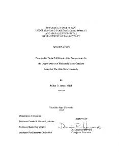
(2.27)

where Fx = (α + 4βπ 2 q 2 ) sin2 (πq sin(θ)) Fy = (α + 4βπ 2 q 2 ) sin2 (πq cos(θ)) It could be derived directly from Eqs. (2..1)–(2..3). Expanding Eq. (2..28) in a Fourier series, we have 2 √ χπq 2 √ ) sin( − (α + 4βπ 2 q 2 )2 (1 − J0 (2πq)) + (α + 4βπ 2 q 2 )2 [2πq(4π 2 q 2 − 24) δ= χ 2 J0 (2πq) − 8(4π 2 q 2 − 6)J1 (2πq)]/(4π 3 q 3 ) · cos(4θ) + O(cos(8 θ)) (2.28) where Jn (x) denotes the n-th order first kind Bessel function. The DC (isotropic) term in Eq. (2..28) introduces a uniform error for all angles and the cos(4θ) term leads to anisotropic errors. The contribution of the higher order cos(nθ) terms is much smaller compared to the cos(4θ) term, and therefore, the isotropic term plus the cos(4θ) terms essentially determine the angular behavior of the numerical dispersion. As an example, Fig. 2.1 and Fig. 2.2 show the isotropic term and the cos(4θ) term of the dispersion error δ, when inserting Eq. (2..24) into Eq. (2..28), optimized for 15o . By changing the optimized angle, the isotropic term changes from nearly zero at 22.5o to nearly 0.0085 at 45o while the cos(4θ) term remains about the same as the one depicted in Fig. 2.2. 13

−3

0

x 10

−0.2

Isotropic term of δ

−0.4

−0.6

−0.8

AO−FDTD optimized at 15 degree (2,4) scheme −1

−1.2 0.01

0.02

0.03

0.04

0.05 0.06 q: wavelengths per cell

0.07

0.08

0.09

0.1

Figure 2.1: Isotropic term of the numerical dispersion error δ.

In fact, in terms of the inf-sup (minimum maximum) numerical dispersion, the AO-FDTD optimized at 22.5o is an optimized one. This can be shown by making the term (α + 4βπ 2 q 2 ) to be a unknown, say ν, and solve for it by enforcing the isotropic term in Eq. (2..28) to be zero, which leads to √ cos( 2πqχ) − 1 ν= χ2 (J0 (2πq) − 1)) By expanding ν in a Taylor series in terms of q, we obtain ν =1+

(3 − 2χ2 )π 2 q 2 24

Note that at 15o , the anisotropic term will almost cancel out the isotropic term. For the filtered schemes, the overall behavior is quite similar. The ordinary Yee’s FDTD scheme is a special case when α = 1 and β = 0 so that at χ = 1.0, it will be automatically optimized (zero dispersion) for 45o from Eq. (2..24). Indeed, the 14

−4

9

x 10

AO−FDTD optimized at 15 degree (2,4) scheme

8

7

cos(4θ) term of δ

6

5

4

3

2

1

0 0.01

0.02

0.03

0.04


0.07

0.08

0.09

0.1

Figure 2.2: cos(4θ) term of the numerical dispersion error δ.

anisotropy of the AO-FDTD scheme is expected to be the same order as the ordinary FDTD (no improvement on this aspect). For the higher-order (2,4) FDTD scheme introduced in [13], we could obtain a dispersion error similar to Eq. (2..28) and proceed with a similar analysis as before. The dispersion error for this (2,4) FDTD scheme is expressed as √ 2 χπq 2 √ δ= sin( 2 ) − [730 − 783J0 (2πq) + 54J0 (4πq) − J0 (6πq)]/576 + {6πq χ [2349(π 2 q 2 − 6)J0 (2πq) + 81(3 − 2π 2 q 2 )J0 (4πq) + (3π 2 q 2 − 2)J0 (6πq)] +28188(3 − 2π 2 q 2 )J1 (2πq) + 243(8π 2 q 2 − 3)J1 (4πq) − 4(6π 2 q 2 − 1) J1 (6πq)}/(5184π 3 q 3 ) · cos(4θ) + O(cos(8 θ)) (2.29) Fig. 2.1 and Fig. 2.2 also depict the isotropic and the cos(4θ) terms of the the (2,4) FDTD dispersion error as a function of q when evaluating Eq. (2..29) for 0.01 ≤ q ≤ 0.1 at χ = 0.85 [13]. For this higher-order scheme, we observe that the cos(4θ) term is (designed to be) much smaller than the isotropic term. 15

2.2.6

Numerical Results

In this section, we compare in more detail the AO-FDTD method with a regular FDTD method and the higher-order (2,4) scheme. Both Butterworth, Chebyshev and non-filtered angle selection schemes are tested at 0o , 15o and 22.5o with χ = 0.74. We use a Butterworth filter with δ expanded to the p = 6 order. The central frequency is such that q0 = 0.08. Furthermore, for the Chebyshev filter we use ∆q = 0.02. The corresponding coefficients are:

Butterworth θ0 = 0o Butterworth θ0 = 15o Chebyshev θ0 = 0o Chebyshev θ0 = 15o Non-filtered θ0 = 15o Non-filtered θ = 22.5o

α β 0.999774 0.032036 0.999843 0.0262875 0.99978 0.0321267 0.999847 0.02635 1.0 0.02505 1.0 0.0198417

Table 2.1: Some coefficients used in 2-D AO-FDTD. The phase velocity in free space is directly simulated in a 2-D FDTD grid. The FDTD domain is large enough so that any spurious reflections from the grid boundary are causally isolated from the results presented here. Moreover, the results are √ normalized to c = 1/ µ0 0 , and χ = 1 for ordinary FDTD and χ = 0.85 for the (2,4) scheme. From Fig. 2.3 and Fig. 2.4, we observe that the AO-FDTD scheme yields almost no numerical dispersion at the optimized angle on a wide range of frequencies around the central frequency. For comparison, Fig. 2.5 depicts the normalized phase velocity of ordinary FDTD for the same frequency range. On the other hand, we see from Fig. 2.6 that the (2,4) scheme yields a highly isotropic result, but with larger absolute errors. Moreover, through a comparison of AO-FDTD results with ordinary FDTD 16

1.007

0 degree 15 degree 30 degree 45 degree

1.006

Relative error of normalized phase velocity

1.005

1.004

1.003

1.002

1.001

1

0.999

0.998

0.997 0.05

0.06

0.07

0.08 q: wavelengths per cell

0.09

0.1

0.11

Figure 2.3: Normalized phase velocity of AO-FDTD scheme optimized at 15o using Butterworth filter

results in finer meshes (Fig. 2.7 vs. Figs. 2.9 –2.10), we observe that the cell size would need to be reduced around at least 5 times to obtain a dispersion error around the optimized angle as small as the non-filtered AO-FDTD. In the case of (2,4) scheme, a mesh approximately 3 times finer would be required (Fig. 2.8 vs. Figs. 2.9–2.10) to reduce to error to the levels presented by the non-filtered AO-FDTD. For filtered AO-FDTD these factors will be even larger. Fig. 2.9 shows the results for a non-filtered AO-FDTD scheme optimized at 22.5o . The numerical dispersion is almost symmetric around this angle. By comparing this result with Figs. 2.3–2.5, we see the anisotropic behavior follows the same pattern, but with a smaller maximum error, as discussed in the Section VI. Fig. 2.10 compares the relative error on the normalized phase velocity for the AO-FDTD with Butterworth filter, Chebyshev filter and the non-filtered AO-FDTD

17

1.009

1.008



1.007

1.006

1.005

1.004

1.003

1.002

1.001

1

0.999 0.05

0.06

0.07


0.09

0.1

0.11

Figure 2.4: Normalized phase velocity of AO-FDTD scheme optimized at 0o using Butterworth filter

scheme. In this figure, the relative errors are the absolute differences between normalized phase velocities and 1.0. Notice that the real (optimal) center frequency for Butterworth filter shifts slightly towards the low frequency end, as explained before. The Chebyshev filter performs best and its actual optimal frequency is almost exactly as the center frequency specified theoretically, q0 = 0.08. Finally, Fig. 2.11 presents the relative error on the normalized phase velocity for four different angles around the optimized angle. A Chebyshev filter optimized at 0o is used. In the vicinity of the optimized angle, we see that the AO-FDTD with Chebyshev filtering works very well: an error no larger that 0.09% is obtained in a angular sector as large as 20o in this case.

18

1.001

1


0.999

0.998

0.997

0.996

0.995


0.994

0.993

0.992

0.991 0.05

0.06

0.07


0.09

0.1

0.11

Figure 2.5: Normalized phase velocity of ordinary FDTD method

2.3 2.3.1

Three-Dimensional AO-FDTD Algorithm Update Equations and Stability Analysis

We introduce a modified set of Maxwell’s curl equations as follows

([T ] · ∇) × E = − ∂∂tB

([T ] · ∇) × H =

(2.30)

∂D ∂t

where ([T ] · ∇) denotes the dot product of vector differential operator ∇ and an artificial correction tensor [T ] defined as  ∆x2 ∂ 2 0 0 α − β v2 t p  2∂2 ∆y 0 0 α − β v2 t [T ] =   p ∆z 2 ∂ 2 0 0 α − β v2 t

   

(2.31)

p

in which ∆x, ∆y and ∆z are the cell size along x, y and z directions respectively, √ vp = 1/ µε is the exact (continuum) phase velocity in the medium, and α and β are additional degrees of freedom in the equations. These parameters are to be 19

1.006

1.0055



1.005

1.0045

1.004

1.0035

1.003

1.0025

1.002

1.0015

1.001 0.05

0.06

0.07


0.09

0.1

0.11

Figure 2.6: Normalized phase velocity of (2,4) FDTD scheme

determined in order to control phase correcting (higher-order) time derivative terms. Such an artificial correction tensor is designed so as to introduce artificial dispersion effects which compensate for the numerical dispersion. Second order time derivatives terms can also be written in terms of the second order space derivatives via the Helmholtz equation [8]. Again, vector wave equations should be used in general. Thus Eq. (2..31) becomes   α − β∆x2 ∇2 0 0  0 α − β∆y 2 ∇2 0 [T ] =  2 2 0 0 α − β∆z ∇

(2.32)

Implementing Eq. (2..32) in the staggered FDTD grid with central differencing in space and a leap-frog discretization in time, we obtain fully discrete update equations for the AO-FDTD. For example, the Ex update is written as l+ 1 ,m,n

Ex i+12

l+ 21 ,m,n

= Ex i

+

∆t ∆y 2 ∆y 2 ∆y 2 l+ 1 ,m+ 12 ,n l+ 1 ,m− 12 ,n −Hz i+ 21 )−β[ 2 {[α+β(3+2 2 +2 2 )](Hz i+ 21 2 2 ∆y ∆x ∆z ∆x 20

1


0.9998

0.9996

0.9994

0.9992

0.999


0.9988

0.9986 0.02

0.025


0.04

0.045

Figure 2.7: Normalized phase velocity of ordinary FDTD method in a finer mesh.

∆y 2 l+ 21 ,m+ 12 ,n+1 l+ 21 ,m− 12 ,n+1 (H −H 1 z z i+ 2 i+ 12 2 2 2 2 ∆z 2 ∆z 2 ∆t l+ 21 ,m+ 12 ,n−1 l+ 21 ,m− 12 ,n−1 l+ 21 ,m+ 32 ,n l+ 21 ,m− 32 ,n {[α+β(3+2 2 +Hz i+ 1 −Hz i+ 1 )+(Hz i+ 1 −Hz i+ 1 )]}− 2 2 2 2 ∆z ∆x l+ 3 ,m+ 12 ,n

(Hz i+ 21

+2

l+ 3 ,m− 12 ,n

−Hz i+ 21

l− 1 ,m+ 12 ,n

+Hz i+ 21

l− 1 ,m− 12 ,n

−Hz i+ 21

)+

∆z 2 ∆z 2 l+ 21 ,m,n+ 12 l+ 21 ,m,n− 12 l− 21 ,m,n+ 12 l− 1 ,m,n− 12 l+ 3 ,m,n+ 12 )](H −H )−β[ −Hy i+ 21 +Hy i+ 21 y i+ 1 y i+ 1 2 2 (Hy i+ 1 2 2 2 2 2 ∆y ∆x l+ 23 ,m,n− 12

−Hy i+ 1 2

∆z 2 l+ 1 ,m−1,n+ 12 l+ 1 ,m−1,n− 12 l+ 1 ,m+1,n+ 12 l+ 1 ,m+1,n− 12 )+ 2 (Hy i+ 21 −Hy i+ 21 +Hy i+ 21 −Hy i+ 21 )+ 2 2 2 2 ∆y l+ 1 ,m,n+ 32

(Hy i+ 21 2

l+ 1 ,m,n− 32

− Hy i+ 21 2

)]}

where the superscripts denote the spatial location of the field components and the subscripts denote the time step. The other update equations are similar. To analyze the stability of the AO-FDTD method, we employ a Von Neumann analysis [63]. The E and H fields are expanded into Fourier modes. For each mode

21

1.001


1.0009


1.0008

1.0007

1.0006

1.0005

1.0004

1.0003

1.0002

1.0001 0.02

0.025


0.04

0.045

Figure 2.8: Normalized phase velocity of (2,4) FDTD scheme in a finer mesh.

l+ 21 ,m,n

1

Ex i

= Ex i (t)e−j[kx (l+ 2 )∆x+ky m∆y+kz n∆z]

Ey i

= Ey i (t)e−j[kx l∆x+ky (m+ 2 )∆y+kz n∆z]

Ez i

= Ez i (t)e−j[kx l∆x+ky m∆y+kz (n+ 2 )∆z]

l,m+ 12 ,n l,m,n+ 12

l,m+ 12 ,n+ 12

1

1

1

1

Hx i+ 1

= Hx i+ 1 (t)e−j[kx l∆x+ky (m+ 2 )∆y+kz (n+ 2 )∆z]

H

= Hy i+ 1 (t)e−j[kx (l+ 2 )∆x+ky m∆y+kz (n+ 2 )∆z]

2 l+ 21 ,m,n+ 12 y i+ 1 2 l+ 21 ,m+ 12 ,n z i+ 1 2

H

(2.33)

2

1

2

1

1

1

= Hz i+ 1 (t)e−j[kx (l+ 2 )∆x+ky (m+ 2 )∆y+kz n∆z] 2

Substituting Eq. (2..33) into the discrete update equations, we obtain the system amplification matrix as        

2 2 ξC + Cxz ξCxy Cyz 0 ζCxy −ζCxz 1 − ξ Cxy xz2 Cyz 2 ξC ξCxz Cyz 1 − ξ Cxy + Cyz C −ζC 0 ζCyz xy xy2 xz 2 ζCxz −ζCyz ξCxy Cyz ξCxy Cxz 1 − ξ Cyz + Cxz 0 γCxz 1 0 0 0 −γCxy 0 −γCyz 0 1 0 γCxy γCyz 0 0 0 1 −γCxz (2.34)

22

       

1.005


1.004


1.003

1.002

1.001

1

0.999

0.998

0.997

0.996

0.995 0.05

0.06

0.07


0.09

0.1

0.11

Figure 2.9: Normalized phase velocity of AO-FDTD scheme optimized at 22.5o using non-filtered scheme

where 4∆t2 , µ

ζ = 2j ∆t , γ = 2j ∆t µ

3kz ∆z β 1 ∆z 2 ∆z 2 sin + 2 sin kz2∆z α + β 3 + 2 ∆y sin kz2∆z − ∆z Cxy = ∆z 2 + 2 ∆x2 2

2 ∆z ∆z 2 cos(k ∆x) + cos (k ∆y) x y 2 2 ∆x ∆y

(2.35) 2 2 k ∆y 3k ∆y ky ∆y ∆y ∆y β y y 1 Cxz = ∆y α + β 3 + 2 ∆x2 + 2 ∆z2 sin − ∆y sin + 2 sin 2 2 2

2 2 ∆y ∆y cos (kx ∆x) + ∆z2 cos (kz ∆z) ∆x2 (2.36)

kx ∆x 3kx ∆x kx ∆x β 1 ∆x2 ∆x2 Cyz = ∆x α + β 3 + 2 ∆y2 + 2 ∆z2 sin 2 − ∆x sin + 2 sin 2 2

2 2 ∆x cos (ky ∆y) + ∆x cos (kz ∆z) ∆y 2 ∆z 2 (2.37) ξ=

The eigenvalues of the system amplification matrix in Eq. (2..34) are λ = 1, λ = 1 −

23

Ξξ±

√

Ξ(Ξξ 2 −4ξ) 2

−4

5

x 10

4.5

Non−filtered Butterworth Chebyshev


4

3.5

3

2.5

2

1.5

1

0.5

0 0.04

0.05

0.06


0.08

0.09

0.1

Figure 2.10: Comparison of Butterworth, Chebyshev and non-filtered AO-FDTD schemes at 15o

with Ξ = Cxy 2 + Cxz 2 + Cyz 2 For the algorithm to be stable, we require |λ| ≤ 1. Thus √ ∆t ≤ 1/(vp Ξ)

(2.38)

When α = 1, β = 0, this reduces to the usual Courant condition. Considering ∆x = ∆y = ∆z = h, the largest possible value of |Cxy |, |Cxz | and |Cyz | is (α + 12β)/h. Thus ∆t ≤ √

h 3vp (α + 12β)

24

(2.39)

−4

9

x 10


8

0 degree 2.5 degree 7.5 degree 10 degree

7

6

5

4

3

2

1

0 0.05

0.06

0.07


0.09

0.1

0.11

Figure 2.11: Relative error of normalized phase velocity around 0o for the AO-FDTD using Chebyshev filter

2.3.2

Optimal Angle Selection

Assuming a monochromatic wave propagating in a uniform grid, then the time dependent parts of Eq. (2..33) can be written as

1

E i (t) = Ee j ω(i∆t) H i+ 1 (t) = He j ω(i+ 2 )∆t

(2.40)

2

Substituting Eq. (2..33) and Eq. (2..40) again into the update equations and eliminating all H field variables, we get  sin2 ω∆t ( 2 ) 2 2 C˜xz C˜yz − C˜xz − C˜xy 2 ∆t2 v p   sin2 ( ω∆t 2 ) 2 2  C˜xz C˜yz − C˜xy − C˜yz vp2 ∆t2  C˜xy C˜yz C˜xy C˜xz

C˜xy C˜yz C˜xy C˜xz sin2 ( ω∆t 2 ) 2 2 − C˜xz − C˜yz v 2 ∆t2



   Ex   Ey  = 0  Ez

p

(2.41)

25

where C˜xy = Cxy |kx =k sin(θ) cos(φ),ky =k sin(θ) sin(φ),kz =k cos(θ),∆x=∆y=∆z=h C˜xz = Cxz |kx =k sin(θ) cos(φ),ky =k sin(θ) sin(φ),kz =k cos(θ),∆x=∆y=∆z=h C˜yz = Cyz |kx =k sin(θ) cos(φ),ky =k sin(θ) sin(φ),kz =k cos(θ),∆x=∆y=∆z=h k=

2 kx + ky2 + kz2 and (θ, φ) are polar angles along which the wave propagates. For

E x , E y and E z to admit nontrivial, the determinant of the matrix in Eq. (2..41) must be zero. Thus we obtain the dispersion relation √ 2 3 χkh 2 2 2 = h2 (C˜xy + C˜xz + C˜yz ) sin √ χ 2 3 √ where χ = vp ∆t 3/h is the Courant (or CFL) number.

(2.42)

Note that in deriving Eq. (2..42), we have implicitly assumed k = ω/vp . Therefore for given (θ, φ) and χ, the error in the discrete phase velocity can be made zero if α and β are properly chosen. In other words, we can solve for α and β from Eq. (2..42) for given (θ, φ) and χ. In order to do this, we first define the error √ 2 χkh 3 2 2 2 − h2 (C˜xy + C˜xz + C˜yz ) δ= sin √ χ 2 3

(2.43)

Solving Eq. (2..42) is equivalent to letting δ = 0. By noting that kh = 2πh/λ, we may expand δ in series in terms of the reciprocal of the number of cells per wavelength, q = h/λ, as: 4 4

δ = (1 − α2 )π 2 q 2 + π288q {63α2 − 2304αβ − 32χ2 + 3α2 [4 cos(2θ) + 7 cos(4θ) +8 cos(4φ) sin4 (θ)]} + O(q 6 ) (2.44) where, in practice, q ≤ 0.1. To solve for α and β, we force the first two terms in Eq. (2..44) to be zero. The resulting error will be O(q 6 ). Thus α = 1.0, β =

63−32χ2 +12 cos(2θ)+21 cos(4θ)+24 cos(4φ) sin4 (θ) 2304

26

(2.45)

For 0 ≤ β < 1/24, the minimum (for all angles) maximum χ for a stable scheme is found from Eq. (2..39) and Eq. (2..45) to be 2/3. This is the CFL number which can be used to minimize the dispersion error for any angle with guaranteed stability. In reality, the CFL number can be made larger than 2/3 depending on the specific α and β. Note that the angular dependency on (θ, φ) only appears in β, which controls the higher order time derivative term and hence the reason why this AO-FDTD scheme could be used for arbitrary angle selection. By using the filtering technique discussed in the previous section, we can also improve the results. This will be shown in the next subsection.

2.3.3

Numerical Experiments

For a particular choice of α and β in Eq. (2..31), the actual phase velocity vp of AO-FDTD simulations can be solved as function of frequency and propagation angle directly from Eq. (2..42), as traditionally done in FDTD dispersion analysis. In this way, the AO-FDTD will be compared with the regular FDTD method (Yee’s scheme) and a scheme with second order of accuracy in time and fourth order of accuracy in space ((2,4) scheme) [12]. Butterworth, Chebyshev and non-filtered AO-FDTD schemes are tested at θ = 90o and φ = 0o (i.e., positive x-direction)1 , with χ = 2/3. √ Moreover, the results are normalized to c = 1/ µ . χ = 1 is used for ordinary FDTD and χ = 6/7 for the (2,4) scheme (maximum respective CFL numbers). The coefficients used here are listed in Table 3.2 and Table 3.3. Figs. 2.12 and 2.13 show the normalized phase velocity of Butterworth and Chebyshev AO-FDTD schemes at θ = 90o and φ = 0o with different specification of center 1

As in 2-D case, it can be shown that the dispersion error along all positive and negative axes are simultaneously optimized.

27

Table 2.2: Some coefficients used in 3-D AO-FDTD.

α β

Non-filtered Butterworth Butterworth Butterworth qc = 0.1 qc = 0.09 qc = 0.08 1 0.999319 0.999562 0.999732 0.0354938 0.0389119 0.0382103 0.0376044

Table 2.3: Coefficients used in the AO-FDTD with Chebyshev filtering scheme. ∆q = 0.02 for all Chebyshev filters.

α β

Chebyshev qc = 0.1 0.999368 0.0388736

Chebyshev qc = 0.09 0.999591 0.0382207

Chebyshev qc = 0.08 0.999748 0.0376482

frequencies. The results are similar for these two schemes. In consonance with filter theory [49], we observe that the Butterworth filter gives slightly more accurate results than the Chebyshev filter at the specified center frequencies, while the Chebyshev filter produces a smaller maximum error than the Butterworth filter in frequency band shown, 0.01 ≤ q ≤ 0.1 (and indeed not limited to ∆q = 0.02 from the filter specification). Note that in Fig. 2.12, the normalized phase velocities are not exactly 1.0 at the center frequencies and this discrepancy tends to increase as the center frequency increases. This phenomena is due to using a finite number of terms in the transformation of basis from q n to {(q − qc )n }. Theoretically, this error could be minimized by increasing the computation overhead when building the filters. Alternatively, we can in practice simply shift the center frequency slightly downward (e.g., optimizing at qc = 0.09 instead of at qc = 0.1). An interesting point to observe in connection with Figs. 2.12-2.13 is that the local dispersion error is actually smaller for higher frequencies (closer to qc ) than for lower 28

1.0001

1

Normalized phase velocity

0.9999

0.9998

0.9997

0.9996

0.9995

Optimized at q =0.08 c Optimized at qc=0.09 Optimized at qc=0.10

0.9994

0.9993 0.01

0.02

0.03

0.04


0.07

0.08

0.09

0.1

Figure 2.12: Normalized phase velocity of Butterworth AO-FDTD scheme at θ = 90o and φ = 0o with different specification of center frequencies

frequencies (as opposed to traditional FDTD schemes). This is highly desirable in practice since at high frequencies the computational domain (of fixed physical size) is electrically larger than at low frequencies and hence the accumulated phase error form the FDTD simulations tends to be larger. With this in mind, qc may also be chosen close to the maximum frequency of interest. Fig. 2.14 shows the comparison of different AO-FDTD schemes, where all filtering schemes are optimized with qc = 0.09. We observe that filtering schemes indeed yield much better results than non-filtered scheme around designed frequencies, where the numerical dispersion is the most critical. Moreover, in the whole frequency range being considered, the maximum errors from both filtering schemes are also smaller than non-filtered scheme. Fig. 2.15 shows the normalized phase velocity of ordinary FDTD and (2,4) schemes. Compared with non-filtered AO-FDTD scheme, approximately 5 29

1.0001

1


0.9999

0.9998

0.9997

0.9996

Optimized at qc=0.08 Optimized at qc=0.09 Optimized at q =0.10

0.9995

c

0.9994

0.9993 0.01

0.02

0.03

0.04


0.07

0.08

0.09

0.1

Figure 2.13: Normalized phase velocity of Chebyshev AO-FDTD scheme at θ = 90o and φ = 0o with different specification of center frequencies

times and 3 times finer meshes would be required for the same accuracy at θ = 90o and φ = 0o , respectively. If compared with filtering schemes, even finer meshes would be required. Finally, Fig. 2.16 illustrates the behavior of the dispersion error as a function of angle (anisotropy). A Butterworth filter optimized at qc = 0.09 is used. The normalized phase velocity is presented for four different elevation angles close to a given optimized angle θc = 90o . The azimuthal angle is fixed at φc = 0o . Note that the numerical dispersion here is rotational symmetric about each coordinate axis, and the results for θc − θ are the same as θ − θc . In the vicinity of the optimized angle, we see that the AO-FDTD works as intended: an error no larger that 0.06% is obtained in a angular sector as large as 15o around the optimized angle.

30

1.0001

1


0.9999

0.9998

0.9997

Non−filtered Butterworth Chebyshev

0.9996

0.9995

0.9994

0.9993 0.01

0.02

0.03

0.04


0.07

0.08

0.09

0.1

Figure 2.14: Normalized phase velocity of Butterworth, Chebyshev and non-filtered AO-FDTD schemes at θ = 90o and φ = 0o . For the filtered schemes, qc = 0.09

We next simulate a ultra wideband pulse propagation to illustrate the effectiveness of the angle optimization in reducing the pulse distortion caused by the numerical dispersion. The source is a zˆ directed electric dipole excited by a first-order differentiated Gaussian pulse centered at 7.5 GHz and having -10 dB points at about 1.5GHz and 16GHz. The medium is free-space and the computation domain is large enough so that any spurious reflection from the grid boundaries are causally isolated from the results presented below. The discretization cell size corresponds to 10 cells per wavelength at 10 GHz. The observation point is at 38 cells away from the source at an angle θ = 90o and φ = 0o , for which the optimization is chosen for the 3-D AO-FDTD. The co-polarized component of the electric field at the observation point is illustrated in Fig.2.17. The largest possible Courant numbers are used in each case, i.e. 1 for Yee’s scheme and 2/3 for AO-FDTD scheme. As a result of the much smaller 31

1.001

1.0005


1

0.9995

0.999

0.9985

0.998

Yee scheme (2,4) scheme

0.9975

0.997 0.01

0.015

0.02

0.025 0.03 0.035 q: wavelengths per cell

0.04

0.045

0.05

Figure 2.15: Normalized phase velocity of ordinary FDTD and (2,4) scheme at θ = 90o and φ = 0o .

numerical dispersion, the AO-FDTD pulse exhibits significantly less distortion that the Yee’s pulse.

2.4

Concluding Remarks

Although not detailed here, the modification on the dispersion behavior of Maxwell’s equations given by Eq. (2..30) could also have been effected, in a dual formulation, entirely in terms of a change on the constitutive parameters of the background medium. In this dual formulation, Maxwell’s equations are not changed, and the background medium becomes a dispersive and anisotropic medium. The dispersive and anisotropic properties of the artificial background media is such that they act to compensate for the dispersive and anisotropic properties of wave propagation caused by the discrete grid. 32

1.0008

θ=90 degree θ=87.5 degree θ=85 degree θ=82.5 degree

1.0006


1.0004

1.0002

1

0.9998

0.9996

0.9994 0.01

0.02

0.03

0.04


0.07

0.08

0.09

0.1

Figure 2.16: Comparison of the normalized phase velocity at different angles of Butterworth AO-FDTD scheme. The center frequency is such that qc = 0.09 1.2

FDTD AO−FDTD Analytical

1

0.8

Normalized magnitude

0.6

0.4

0.2

0

−0.2

−0.4

−0.6

−0.8

0

1

2

3

4 Time(s)

5

6

7

8 −10

x 10

Figure 2.17: Simulated results of a first-order differentiated Gaussian pulse propagating at θ = 90o and φ = 0o

33

CHAPTER 3

DISPERSION-RELATION-PRESERVATION FDTD SCHEMES

3.1

Introduction

In recent years, several techniques have been developed to reduce numerical dispersion error in finite-difference solutions. Among these, the Cole’s non-standard finite-difference (NSFD) [9] and Forgy’s scheme [15] have particularly low dispersion error for narrow-band simulations [59]. Moreover, various high order schemes based on traditional Yee’s staggered grids have been proposed for broadband simulations. Traditional fourth order of accuracy in time and fourth order of accuracy in space schemes [so called (4,4) schemes], including the ones proposed independently by Fang [12] and Deveze [11] are particularly attractive for such problems [23],[58],[59]. Since the ability to solve broadband problems is a main motivation for using time domain methods, it is important to develop FDTD algorithms with reduced dispersion error in a broadband range. On this aspect, it is important to notice that, for many practical FDTD simulations, the minimization of the local and accumulated dispersion error over a finite range of frequencies is often more relevant than the theoretical order of accuracy of the FDTD scheme itself, where order of accuracy refers to the (truncation) error of the scheme as the grid spacing goes to zero (very 34

low frequency or long wavelength limit). This is because of two (interconnected) main reasons: (1) The very low frequency limit is often not that relevant in practice, unless in the case of quasi-static simulations or in simulations where some kind of very fine adaptive grid refinement is employed. Indeed, in the majority of FDTD simulations of wave propagation problems, the spectral energy is mostly within wavelengths on the order of 101 ∆ − 102 ∆, where ∆ is the grid discretization size. (2) FDTD simulations involve computational domains of fixed physical size. In the very low frequency limit, the computational domain is electrically smaller and, therefore, the accumulated phase error (which grows linearly with the electric size of the domain) is less of a problem. One relevant question then arises on how to construct optimal FDTD algorithms with dispersion-relation-preserving (DRP) properties on a given (possibly wide) frequency band. Because of its cumulative effect, high frequency components are subject to a larger cumulative phase error than low frequency components. Thus it is also of interest to investigate the possibility of constructing FDTD algorithms such that the (local) dispersion error incurred is lower for high frequencies than for low frequencies (in traditional schemes usually the opposite is true). In this chapter, we shall describe a methodology to develop DRP schemes for both 2-D and 3-D FDTD algorithms with these observations in mind. Although our main motivation is for time-domain broadband problems, the proposed methodology is suited to minimize the dispersion error at specific frequencies.

35

3.2 3.2.1

Two-Dimensional DPR-FDTD Algorithm Methodology

Because the dispersion error is in general a function of both frequency, propagation angle, and the particular Courant-Friedrichs-Lewy (CFL) number, several definitions of minimum dispersion error [45], [23] are possible. We define it here in the minimax (minimum maximum) sense, i.e., for a given CFL number, the maximum dispersion error for all angles is minimized up to a certain frequency. The DRP procedure here consists of three main steps: 1) For a scheme with given “order of accuracy in space”, the dispersion error is expanded in a Fourier series in terms of the propagation angle, and analytical expressions for the DRP coefficients are subsequently derived as a function of frequency. 2) These analytical expressions are then cast into a form implementable in the fully-discrete problem (FDTD method) by using polynomial expansions. 3) If necessary, filtering schemes (maximally flat or Chebyshev) are used to fine-tune the DRP 2-D FDTD coefficients for a pre-assigned frequency range. The first step consists in considering a scheme with a given “order of accuracy in space”. Higher order of accuracy in time is introduced in the second step as we expand the analytical solution in series. The term “order of accuracy in space” is borrowed here from traditional higher order schemes employing Taylor expansions only [12], [11]. Since this work treats the problem from a different standpoint, this term does not retain its original meaning. The term order of accuracy should be considered here as referring to a class of spatial stencil sizes and not necessarily to the precise order of the truncation error as the discretization cell size goes to zero. As we will see, the major difference between the DRP higher order schemes derived

36

here and traditional higher order schemes resides in the coefficients and not on the particular FDTD stencil. Non-filtered, DRP (2,2) Schemes A traditional leap-frog scheme with second order of accuracy in space can be written in general as: Ex l+1 = Ex lm+ 1 ,n + m+ 1 ,n 2

2

∆t l+ 1 l+ 1 Γx (Hz m+2 1 ,n+ 1 − Hz m+2 1 ,n− 1 ) 2 2 2 2 ∆y

(3.1)

∆t l+ 1 l+ 1 (3.2) Γy (Hz m−2 1 ,n+ 1 − Hz m+2 1 ,n+ 1 ) 2 2 2 2 2 2 ∆x ∆t ∆t l− 1 = Hz m+2 1 ,n+ 1 + Γx (Ex lm+ 1 ,n+1 −Ex lm+ 1 ,n )+ Γy (Ey lm,n+ 1 −Ey lm+1,n+ 1 ) 2 2 2 2 2 2 µ∆y µ∆x (3.3) = Ey lm,n+ 1 + Ey l+1 m,n+ 1

l+ 1

Hz m+2 1 ,n+ 1 2

2

where the subscripts denote the spatial location and the superscripts denote the time step. We treat Γx and Γy as unknowns coefficients for the moment. The E and H fields can be expanded into a discrete set of Fourier modes. For each mode 1

Ex lm+ 1 ,n = E x e j ωl∆t e−j[kx (m+ 2 )∆x+ky n∆y]

(3.4)

2

1

Ey lm,n+ 1 = E y e j ωl∆t e−j[kx m∆x+ky (n+ 2 )∆y]

(3.5)

2

l+ 1

1

1

1

Hz m+2 1 ,n+ 1 = Hz e j ω(l+ 2 )∆t e−j[kx (m+ 2 )∆x+ky (n+ 2 )∆y] 2

2

(3.6)

Substituting (3.4)-(3.6) into (3.1)-(3.3) and noticing that E x = −Esin(θ), E y = Ecos(θ) and Hz = H, we have sin(

k sin(θ)∆y ω∆t ∆t )Esin(θ) = Γx Hsin[ ] 2 ∆y 2

(3.7)

ω∆t k cos(θ)∆x ∆t )Ecos(θ) = Γy Hsin[ ] (3.8) 2 ∆x 2 ω∆t k sin(θ)∆y k cos(θ)∆x ∆t ∆t sin( )H= Γx Esin[ ] sin(θ) + Γy Esin[ ] cos(θ) (3.9) 2 µ∆y 2 µ∆x 2 sin(

37

where kx = k cos(θ), ky = k sin(θ). The numerical dispersion relationship can be derived from (3.7)-(3.9) as Γ2y k cos(θ)∆x Γ2x 1 2 ω∆t 2 k sin(θ)∆y sin ( sin [ sin2 [ )= ]+ ] (3.10) 2 2 2 (vp ∆t) 2 ∆y 2 ∆x 2 √ where vp = µ . For a given set of coefficients Γx and Γy (in Yee’s scheme they are equal to unity), the above equation is traditionally used to analyze the discrete dispersion in the FDTD grid. The amount by which the discrete dispersion relation deviates from the continuum limit gives the local dispersion error. In this work, we shall adopt the reverse standpoint. That is, we shall enforce the exact relation between frequency and wavenumber, viz. ω = vp k, for (3.10), and then solve for Γx and Γy as the unknowns (in an approximate sense to be clear later on). Ideally, the exact solutions for Γx and Γy should depend on both the frequency and propagation angle. We shall first expand the dispersion error in terms of a Fourier series in terms of the angular variable θ and enforce coefficients on the series to be zero (the number of coefficients made equal to zero give the “order” of the method). In this manner, the maximum dispersion error for all angles is minimized simultaneously, and Γx and Γy become a function of frequency only. This latter property allows for incorporation of the DRP coefficients in FDTD algorithms after a polynomial expansion. A simpler but equivalent way of solving for Γx and Γy in (3.10) is to enforce ω = vp k into (3.7) and (3.8) and solve for Γx and Γy , respectively2 . We start by defining an error functional proportional to the difference between l.h.s. and r.h.s. of (3.7)

√ δ2 (Γx , θ) =

2

πqy χy sin( √ ) sin(θ) − Γx sin[πqy sin(θ)] χy 2

2

(3.11)

Note that (from the symmetry of the problem) by letting ∆x → ∆y and θ → θ + π/2, (3.8) reduces to (3.7). In particular if ∆x = ∆y, we should of course expect Γx = Γy after these coefficients are reduced to functions of frequency only.

38

where χy =

√

2vp ∆t/∆y, qy = ∆y/λ. Solving (3.7) with ω = vp k is therefore equiva-

lent to letting δ2 (Γx , θ) = 0 and enforcing E/η = H. We expand δ2 (Γx , θ) in a Fourier series in terms of θ and use the following identities 2π sin[x sin(θ)] cos(nθ)dθ = 0 02π sin[x sin(θ)] sin(nθ)dθ = 2πJn (x) 0 for odd n and

2π sin[x sin(θ)] cos(nθ)dθ = 0 02π sin[x sin(θ)] sin(nθ)dθ = 0 0

for even n, where Jn (x) is the n-th order first kind Bessel function, to force the first non-zero (dominant) term of the series to be zero. This leads to √ Γx = γx(∞) ≡

πqy χy sin( √ )/[2J1 (πqy )] χy 2 2

(3.12) (∞)

Substituting (3.12) in (3.11), the residual error δ2e ≡ δ2 (Γx , θ) − δ2 (γx , θ) is given by δ2e = Γx J3 (πqy ) sin(3θ) + Γx J5 (πqy ) sin(5θ) + ... Note that, since |Jn (x)| < 1/(2n · n!) for |x| < 1, (the inequality πqy < 1 is satisfied in practical FDTD simulations with qy < 0.1), the coefficients in this series decrease very rapidly, as expected. The magnitude of each coefficient in the series represents the maximum dispersion error from the corresponding angular mode (either at sin(nθ)=1 or at cos(nθ) =1). (∞)

It is clear that the solution γx

given in (3.12) cannot be implemented in a time (∞)

domain method. Because of this, we expand γx (∞)

and retain the lowest order terms, i.e., γx γx(2) = 1 +

in a Taylor series around qy = 0

= γx + O(qy4 ) with (2)

1 2 2 4π qy (3 − 2χ2y ) 96 39

(3.13)

The above can be easily transformed back to time domain through ω 2 → −∂ 2 /∂t2 . However, if straightforward time discretization schemes are employed directly on the the resulting equations (with third order time derivatives), the update becomes unconditionally unstable [11]. Alternatively, the second order time derivative can be further cast as a combination of spatial derivatives as vp2 ∇2 (Helmholtz equation) and discretized as such (modified equation method [8]). This latter transformation is valid for staggered grids as long as is uniform in the local stencil. In this manner, (3.13) becomes γx(2) = 1 −

(3 − 2χ2y )∆2y ∇2 96

(3.14)

Following a similar procedure for Γy , we find γy(2) = 1 − where χx =

√

(3 − 2χ2x )∆2x ∇2 96

(3.15)

2vp ∆t/∆x. If only the first order terms in (3.14) and (3.15) are taken,

the Yee’s scheme is recovered. Note that the second terms in (3.14) and (3.15) are the analogous to third order time derivative terms in traditional schemes with fourth order of accuracy in time [11]. To investigate the resulting numerical dispersion, we define a dispersion error functional δ 2 (Γx , Γy , θ) proportional to the difference between the l.h.s. and the r.h.s. of (3.10), i.e., √ δ 2 (Γx , Γy , θ) = where χ = (∞)

γx

√

2 k cos(θ)∆x 2 k sin(θ)∆y 2 ) ) Γ2y sin2 ( πqχ 2 2 2 Γx sin ( 2 + (3.16) sin( √ ) − h χ ∆y 2 ∆x2 2

2vp ∆t/h, q = h/λ, and h = min(∆x, ∆y). By substituting Γx = (∞)

and Γy = γy

(∞)

(∞)

δ 2 (γx , γy

(∞)

into (3.16), we obtain a limit value for the error δ 2 (θ) =

, θ). In practical time domain simulations employing (3.14) and (3.15), 40

(2)

(2)

(2)

we have an error δ 2 (θ) = δ 2 (γx , γy , θ) instead, which inevitably introduces addi(∞)

tional errors at high frequencies. The function δ 2 (θ) therefore serves as a inferior theoretical limit when an infinite Taylor expansion is considered. However, as we shall see in the next subsection, by expanding Γx and Γy in a different basis (e.g., Chebyshev polynomials) this limit can indeed be overcome over some finite, pre-assigned frequency range.

−3

1.6

x 10

1.4

1.2

Analytical 2nd order Yee

δ2

1

0.8

0.6

0.4

0.2

0 0.01

0.02

0.03

0.04


0.07

0.08

0.09

0.1

Figure 3.1: Comparison of the maximum value of the dispersion error δ 2 (Γx , Γy , θ) (∞) (∞) for all angles when using analytical solution, (Γx , Γy ) = (γx , γy ), second order (2) (2) approximation (Γx , Γy ) = (γx , γy ) and Yee’s scheme (Γx , Γy ) = (1, 1).

(∞)

(2)

Fig.3.1 shows the maximum value for all angles of δ 2 (θ) (analytical), δ 2 (θ) (second order), and δ 2 (1, 1, θ) (Yee’s scheme), as a function of the number of wavelengths per cell (or, equivalently, the frequency). In these plots, ∆x = ∆y and the CFL number χ = 3/4 (χx = χy = χ). From this figure, we observe that, for all the 41

frequency range such that qy ≤ 0.1, the second order approximation already gives results almost as accurate as using the analytical expression (3.12), and starts to deviate only slightly at high frequencies close to qy = 0.1. Non-filtered, DRP (2,4) Schemes Traditional FDTD schemes with fourth order of accuracy in space employ larger stencils for the Ex and Ey update equations. In this case, the Ex update can be rewritten as follows (compare with (3.1)) Ex l+1 = Ex lm+ 1 ,n + m+ 1 ,n 2

2

∆t l+ 1 l+ 1 Γx1 (Hz m+2 1 ,n+ 1 − Hz m+2 1 ,n− 1 )+ 2 2 2 2 ∆y

∆t l+ 1 l+ 1 Γx2 (Hz m+2 1 ,n+ 3 − Hz m+2 1 ,n− 3 ) 2 2 2 2 ∆y

(3.17)

We proceed as before and Γx1 , Γx2 can be solved from sin(

vp k∆t k sin(θ)∆y 3k sin(θ)∆y ∆t ∆t )E sin(θ) = Γx1 H sin[ ]+ Γx2 H sin[ ] (3.18) 2 ∆y 2 ∆y 2

To obtain Γx1 and Γx2 , we define an error functional in terms of the difference between the l.h.s. and r.h.s. of (3.18) √ δ4 (Γx1 , Γx2 , θ) =

πqy χy sin( √ ) sin(θ) − Γx1 sin[πqy sin(θ)] − Γx2 sin[3πqy sin(θ)] χy 2 (3.19) 2

Similarly as before, we expand δ4 (Γx1 , Γx2 , θ) in a Fourier series in terms of θ. However, since there are two unknowns Γx1 and Γx2 , we now may force the first two non-zero terms of the series to be zero (sin(θ) and sin(3θ) terms). The solutions are given by √ 2 sin( πq√y2χy )J3 (3πqy ) (∞) Γx1 = γx1 ≡ (3.20) 2χy [J1 (πqy )J3 (3πqy ) − J1 (3πqy )J3 (πqy )] √ 2 sin( πq√y2χy )J3 (πqy ) (∞) Γx2 = γx2 ≡ (3.21) 2χy [J1 (3πqy )J3 (πqy ) − J1 (πqy )J3 (3πqy )] 42

(∞)

(∞)

With these coefficients, the residual error defined as δ4e ≡ δ4 (Γx1 , Γx2 , θ)−δ4 (γx1 , γx2 , θ) becomes δ4e = Γx1 J5 (πqy ) sin(5θ) + Γx2 J5 (3πqy ) sin(5θ) + ... (∞)

(∞)

For incorporation into the FDTD update, γx1 and γx2 are approximated as (∞)

(2)

(2)

(2)

(3.22)

(∞)

(2)

(2)

(2)

(3.23)

γx1 ≈ γx1 = γx11 − γx12 ∆y 2 ∇2 γx2 ≈ γx2 = γx21 − γx22 ∆y 2 ∇2 with 9 8 3(3 − 4χ2y ) (2) γx12 = − 512 1 (2) γx21 = − 24 (27 − 4χ2y ) (2) γx22 = − 4608 (2)

γx11 =

The lowest order terms in (3.22) and (3.23) recover Fang’s (2,4) FDTD scheme [12]. (2)

(2)

Similarly, γy1 and γy2 write as (2)

(2)

(2)

(3.24)

(2)

(2)

(2)

(3.25)

γy1 = γy11 − γy12 ∆x2 ∇2 γy2 = γy21 − γy22 ∆x2 ∇2 (2)

(2)

with coefficients γyij written as γxij above with χy replaced by χx . (2)

(2)

(2)

(2)

The implementation of γx1 , γx2 , γy1 and γy2 in staggered grids are straightforward. For example, the fully discrete form of (3.17) is Ex l+1 = Ex lm+ 1 ,n + m+ 1 ,n 2

2

l+ 1

∆t ∆y 2 (2) (2) (2) {[γx11 + γx12 (3 + 2 2 ) − γx22 ] ∆y ∆x

l+ 1

(2)

(2)

(Hz m+2 1 ,n+ 1 − Hz m+2 1 ,n− 1 ) + [γx21 + 2γx22 (1 + 2

2

2

2

43

∆y 2 (2) ) − γx12 ] ∆x2

l+ 1

l+ 1

(2)

(Hz m+2 1 ,n+ 3 − Hz m+2 1 ,n− 3 ) − γx12 2

2

l+ 21

2

2

l+ 21

∆y 2 ∆x2

l+ 1

l+ 1

(Hz m− 1 ,n+ 1 + Hz m+ 3 ,n+ 1 − Hz m−2 1 ,n− 1 − Hz m+2 3 ,n− 1 ) 2

2

(2)

2

2

2

l+ 21

2

l+ 21

2

(2)

−γx22 (Hz m+ 1 ,n+ 5 − Hz m+ 1 ,n− 5 ) − γx22 2

l+ 1

2

2

l+ 1

2

l+ 1

2

2

∆y ∆x2 l+ 1

(Hz m−2 1 ,n+ 3 + Hz m+2 3 ,n+ 3 − Hz m−2 1 ,n− 3 − Hz m+2 3 ,n− 3 )} 2

2

2

2

2

2

2

2

The stability condition can be derived in a standard way [63] and the result is 1 ∆t ≤

Dx2 vp ∆y 2 +

Dy2 ∆x2

(3.26)

where ∆y 2 (2) ky ∆y 3ky ∆y (2) [γ sin( sin( ) + γ )] cos(kx ∆x) x12 x22 ∆x2 2 2 5ky ∆y ∆y 2 ky ∆y (2) (2) (2) (2) ) − [γx11 + γx12 (3 + 2 2 ) − γx22 ] sin( ) +γx22 sin( 2 ∆x 2 ∆y 2 3ky ∆y (2) (2) (2) −[γx21 + 2γx22 (1 + ) − γx12 ] sin( ) 2 ∆x 2 Dx = 2

(3.27)

and similarly for Dy . For ∆x = ∆y, (3.26) becomes ∆t ≤

hχ h √ = √ ˜ x,y |max vp 2 vp 2|D

˜ x,y |max denotes the maximum possible module of Dx and Dy . The minimum where |D maximum CFL number χ with guaranteed stability is found to be 48/65. Note that this is a conservative bound. In reality, we have found χ = 0.75 to produce stable updates in our tests. To estimate the optimization quality, an error functional δ 4 (Γx1 , Γx2 , Γy1 , Γy2 , θ) is constructed in an analogous way as the error functional in (3.16). Fig. 3.2 shows the comparison of the largest δ 4 (among all angles) by using different schemes when ∆x = ∆y and χ = 48/65. In this figure, the analytical result refers to the (ideal) 44

(∞)

(∞)

(∞)

(∞)

choice (Γx1 , Γx2 , Γy1 , Γy2 ) = (γx1 , γx2 , γy1 , γy2 ), whereas the second order result refers to the (implementable) approximation for the coefficients given by (3.22)-(3.25), (2)

(2)

(2)

(2)

(Γx1 , Γx2 , Γy1 , Γy2 ) = (γx1 , γx2 , γy1 , γy2 ). Maximally flat and Chebyshev refer to (implementable) approximations using filtering schemes to be detailed in the next section. Filtering Instead of possibly using even higher order terms in the Taylor series or other sophisticated (and more costly) time integration schemes, it is possible to improve the results of the previous section (while maintaining the same spatial stencil sizes and computational cost) by using filters adjusted to some pre-assigned, finite frequency range. The filters are designed to obtain both Γx and Γy (second order stencil), or Γx1 , Γx2 , Γy1 and Γy2 (fourth order stencil). The procedure is essentially the same for all coefficients and therefore, we will describe only the Γx1 case in detail. Maximally Flat (Butterworth) Filters Expanding (3.20) in a Taylor series, and approximating (3.20) in a finite series as in (3.22) noting that ∆y 2 ∇2 = −4π 2 qy2 , we have (∞) (m) γx1 −γx1

=

3π 4 χ2y (2χ2y − 5) 4 3(4χ2y − 3)π 2 9 (m) 2 (m) − γx11 − + 4π γx12 qy2 + qy +O(qy6 ) 8 128 2560 (3.28) (m)

(m)

The superscript (m) in γx11 and γx12 above refer to maximally flat coefficients. Pre(m)

(2)

(m)

(2)

viously, we have simply chosen γx11 = γx11 and γx12 = γx12 so as to make the first and second terms of the right hand side of the above identically zero (and obtain a O(qy4 ) truncation error). These coefficients are treated as unknowns for the moment. 45

The above equation can be rewritten as γx1 − γx1 = (d0 , 0, d2 , 0, d4 ) · V T + O(qy6 ) (∞)

(m)

(3.29)

where 9 (m) − γx11 8 2 3(4χy − 3)π 2 (m) d2 = −[ + 4π 2 γx12 ] 128 3π 4 χ2y (2χ2y − 5) d4 = 2560 d0 =

V = (1, qy , qy2 , qy3 , qy4 ) By expanding the above in a new basis {(qy − qyc )n }, where qyc refers to a center frequency of interest, the following relationship holds QT = A · V T with Q = (1, (q − qyc ), (q − qyc )2 , (q − qyc )3 , (q − qyc )4 )   1 0 0 0 0  −qyc 1 0 0 0    c2 c  −2qy 1 0 0  A =  qy   −qyc 3 3qyc 2 −3qyc 1 0  qyc 4 −4qyc 3 6qyc 2 −4qyc 1

(3.30)

(3.31)

and, therefore, (3.29) can be rewritten as (∞)

(m)

γx1 − γx1

= (d0 , 0, d2 , 0, d4 ) · A−1 · QT + O(qy6 ) = d˜0 , d˜1 , d˜2 , d˜3 , d˜4 · QT + O(q 6 ) y

where (m) d˜0 = {2880 − 2560γx11 + 3π 4 qyc 4 χ2y (2χ2y − 5)

−20qyc 2 [512π 2 γx12 + 3π 2 (4χ2y − 3)]}/2560 (m)

46

(3.32)

(m) d˜1 = qyc π 2 {90 + 3χ2y [π 2 qyc 2 (2χ2y − 5) − 40] − 5120γx12 }/640 (m) d˜2 = π 2 {90 + 3χ2y [3π 2 qyc 2 (2χ2y − 5) − 40] − 5120γx12 }/1280

d˜3 = 3π 4 χ2y qyc (2χ2y − 5)/640 d˜4 = 3π 4 χ2y (2χ2y − 5)/2560 (m) (m) To solve for γx11 and γx12 , we force d˜0 and d˜1 to be zero and obtain

γx11 = [2880 + 3π 4 χ2y qyc 4 (5 − 2χ2y )]/2560

(3.33)

γx12 = 3{30 + χ2y [π 2 qyc 2 (2χ2y − 5) − 40]}/5120

(3.34)

(m)

(m)

which are functions of qyc . Note that, if we let qyc = 0, we recover γx11 = γx11 and (m)

(m)

(2)

(2)

γx12 = γx12 . In this manner, (∞) (m) γx1 − γx1 = [d˜2 (qy − qyc )2 + d˜3 (qy − qyc )3 + d˜4 (qy − qyc )4 ] + O(qy6 )

At the center frequency, qy = qyc and δ = O(qy6 ). The remainder corresponds to a O(qy6 ) error. Around the center frequency, the error is dominated by the d˜2 (qy − qyc )2 (m)

term. In the above, we have illustrated the derivation of γx1 by using a p = 4 order polynomial for the Taylor expansion in (3.29). Theoretically, we can increase indefinitely the polynomial order p at the (one-time) cost of inverting a larger A and hence make the response as close to an exact second-order maximally flat filter response as desired. This has the (one-time) cost of inverting an increasingly larger matrix A. In practice, we observe a fast convergence to the exact filter response since only negligible improvements are obtained for p ≥ 6. We employ p = 10 throughout our numerical simulations. Also in practice, the design frequency qyc may be chosen as the highest frequency of interest. 47

Fig. 3.2 includes the δ 4 error of the DRP scheme with maximally flat filters designed at q c = 0.1 (∆x = ∆y). From this figure, we observe that near the central frequency (q c = 0.1), the δ 4 using a second-order (with p = 10) maximally flat filter is almost indistinguishable from the one using the analytical solutions (3.20) and (3.21).

−5

0

x 10

δ

4

−2

−4

Analytical Non−filtered DRP Maximally Flat DRP Chebyshev DRP −6 0.01

0.02

0.03

0.04


0.07

0.08

0.09

0.1

Figure 3.2: Comparison of the largest δ 4 among all angles by using different DRP schemes for the fourth-order stencil. See text for details.

Chebyshev Filters We may choose {Tn [(qy − qyc )/∆qy ]} as a new basis expansion in (3.30) instead, where Tn (x) is the n-th order first-kind Chebyshev polynomial, and ∆qy corresponds to the frequency band of interest. Still using p = 4 as an example, Eqs. (3.30) and (3.31) now become Q = (1,

qy − qyc qy − qyc qy − qyc qy − qyc , T2 ( ), T3 ( ), T4 ( )) ∆qy ∆qy ∆qy ∆qy 48

     A=   

1

0

− ∆qyy

1 ∆qy 4q c − ∆qy2 y 12qyc 2 −3∆qy2 ∆q 3 16qyc ∆qy2 −32qyc 3 ∆qy4

qc

2qyc 2 −∆qy2 ∆qy2 3qyc ∆qy2 −4qyc 3 ∆qy3 8qyc 4 −8qyc 2 ∆qy2 +∆qy4 ∆qy4

0 0

0 0

2 ∆qy2 12q c − ∆q3y y 48qyc 2 −8∆qy2 ∆qy4

0 4 ∆qy3 32q c − ∆q4y y

 0 0    0    0   8 ∆qy4

Following the same procedure as maximally flat filter case, we can solve for the (c)

(c)

coefficients and obtain γx11 and γx12 of an approximate second-order Chebyshev filter. Here (∞) (c) γx1 − γx1 = dˆ2 T2 [(qy − qyc )/∆qy ] + dˆ3 T3 [(qy − qyc )/∆qy ] + dˆ4 T4 [(qy − qyc )/∆qy ] + O(qy6 )

where dˆ2 , dˆ3 and dˆ4 denote the coefficients of the corresponding Chebyshev polynomials. Since T2 [(qy − qyc )/∆qy ] takes the minimums at qyc and T3 [(qy − qyc )/∆qy ] is zero at qyc , we can obtain an even better accuracy than using the analytical solutions given by (3.20) and (3.21) at a particular design frequency. Fig. 3.2 (with qy = qx = q) clearly shows that δ 4 by using Chebyshev filters designed with q c = 0.1 and ∆q = 0.023 can be smaller than employing (3.20) and (3.21) around the design frequency. For the Chebyshev filter approximation, we have also set p = 10. Since the Chebyshev filter is set to be of second order, larger ripples are expected to occur in the passband q c − ∆q ≤ q ≤ q c + ∆q if a larger ∆q is used [48]. In usual filter design, large ripples are undesired, but in our context, ∆q represents an extra degree of freedom that can be explored to reduce the accumulated phase error. This will be illustrated in the next section. 3

∆q = 0.02 is used here as an example. As shown later, ∆q can be fine-tuned for a better performance.

49

3.2.2

Numerical Results

We compare the DRP (2,2) and (2,4) schemes against the Yee’s scheme, a traditional (2,4) scheme, and Deveze’s (4,4) scheme. Both non-filtered, and the maximally flat and Chebyshev filtered versions of the DRP schemes are considered. The phase velocity in free space is solved from the transcendental dispersion relation by assuming an uniform 2-D FDTD grid with ∆x = ∆y, or Γx = Γy , and, hence, the coordinate subscript in the coefficients is dropped in what follows. The CFL number χ = 1 is used for ordinary FDTD, while χ = 6/7 for the (2,4) scheme, χ = 3/4 for the (2,2) scheme and χ = 48/65 for all (2,4) schemes. In fact, there is an optimal CFL number for each algorithm, which yields the minimum dispersion error among all possible CFL numbers. When comparing different algorithms, we employ their largest possible CFL numbers instead of that optimal one. This choice is justified since the largest CFL number minimizes the computational cost and is the most often used in practice. Table 4.1 and Table 4.2 give some coefficients used in the DRP (2,4) schemes, where the maximally flat filter is designed with q c = 0.1, and the Chebyshev filter is designed with q c = 0.1 with ∆q = 0.02. Table 4.3 and Table 4.4 give the coefficients using Chebyshev filtering schemes for various pairs (qc , ∆q).

Γ11 Γ12 Deveze 1.125 -1.136094e-2 Non-filtered DRP 1.125 4.797060e-3 Maximally Flat DRP 1.125026 4.669305e-3 Chebyshev DRP 1.125025 4.665140e-3

Table 3.1: Coefficients used in different 2-D (2,4) schemes.

50

Γ21 Γ22 Deveze -4.166667e-2 4.207758e-4 Non-filtered DRP -4.166667e-2 -5.386002e-3 Maximally Flat DRP -4.159725e-2 -5.733253e-3 Chebyshev DRP -4.159842e-2 -5.744642e-3

Table 3.2: Coefficients used in different 2-D (2,4) schemes (cont’d). 4

Yee (4,2) DRP scheme (2,4) scheme

3

Phase error/λ (deg)

2

1

0

−1

−2 0.01

0.02

0.03

0.04


0.07

0.08

0.09

0.1

Figure 3.3: Comparison of the maximum (for all angles) phase error per wavelength using Yee’s, a traditional (2,4) scheme and the non-filtered DRP (2,2) scheme.

Fig. 3.3 and Fig. 3.4 show the maximum (for all angles) phase error per waveˆ − 1) ∗ 360 with kˆ denotes the discrete wavenumber obtained by length, defined as (k/k solving the transcendental dispersion relation and k refers to the exact (continuum) wavenumber. As we see from Fig. 3.3, the DRP (2,2) scheme is about as accurate as the (2,4) scheme (with opposite sign). Fig. 3.4 shows that filtering schemes do reduce the dispersion error considerably around the specified frequency. We also observe that the Chebyshev filter performs better than the maximally flat filter in the full 51

0

−0.02


−0.04

−0.06

−0.08

−0.1

Non−filtered DRP Maximally Flat DRP Chebyshev DRP Deveze

−0.12

−0.14 0.01

0.02

0.03

0.04


0.07

0.08

0.09

0.1

Figure 3.4: Comparison of the maximum (for all angles) phase error per wavelength using different DRP (2,4) schemes and the Deveze (4,4) scheme.

frequency range considered. Note that Fig. 3.4 does not correspond to Fig. 3.2 well after the crossover since Fig. 3.2 is just an analytical estimation for design purposes, while Fig. 3.4 depicts the actual performance of the algorithms. We also note from Fig. 3.4 that, for the DRP schemes with filtering, the dispersion error at high frequencies can be made smaller than for low frequencies (contrary to non-filtered DRP and traditional schemes). As mentioned in the Introduction, this is a desirable characteristic because for a given computational domain (fixed physical size), high frequencies correspond to an electrically larger problem and hence are more impacted by the accumulated phase error. Nevertheless, unless the local dispersion error decreases faster than linearly with frequency, the largest accumulated phase error in the computational domain is still given by the highest frequency components. This issue will be further elaborated next. 52

Γ11 q = 0.1, ∆q = 0.02 1.125025 c q = 0.1, ∆q = 0.046 1.125024 q c = 0.1, ∆q = 0.037 1.125024 q c = 0.1, ∆q = 0.058 1.125023 q c = 0.114, ∆q = 0.053 1.125025 c

Γ12 4.665140e-3 4.647156e-3 4.655009e-3 4.633954e-3 4.665140e-3

Table 3.3: Coefficients of Chebyshev filtering schemes and ∆q. Γ21 c q = 0.1, ∆q = 0.02 -4.159842e-2 c q = 0.1, ∆q = 0.046 -4.160251e-2 q c = 0.1, ∆q = 0.037 -4.160091e-2 q c = 0.1, ∆q = 0.058 -4.160454e-2 q c = 0.114, ∆q = 0.053 -4.159842e-2

with different parameters qc Γ22 -5.744642e-3 -5.793854e-3 -5.772360e-3 -5.830010e-3 -5.744642e-3

Table 3.4: Coefficients of Chebyshev filtering schemes with different parameters qc and ∆q(continued). We assume a FDTD simulation in a (typical) frequency range such that the lowest frequency corresponds to q = 0.01 and the highest frequency corresponds to q = 0.1. Now consider the phase error accumulated in a distance which equals to the largest wavelength being considered. Fig. 3.5 shows the largest (for all angles) phase error accumulated in such a distance by employing Chebyshev filtered DRP algorithms with different ∆q (while qc is kept fixed as 0.1). For ∆q = 0.02, the usual notion that the largest accumulated phase error is dominated by the highest frequency is still valid. However, this is not true anymore if larger ∆q are considered. In fact, when ∆q = 0.046, the largest accumulated phase error is now determined by lower frequency components. Indeed, there is an optimal ∆q around ∆q = 0.058 for which the maximum accumulated magnitude of the phase error for all frequencies is a minimum. In the case of narrowband simulations, we can obtain a pair (qc , ∆q) which yields a minimum possible maximum phase error at some specific frequency. As illustrated 53

0.3

∆ q=0.02 ∆ q=0.037 ∆ q=0.046 ∆ q=0.058

Maximum accumulated phase error/λmax (deg)

0.2

0.1

0

−0.1

−0.2

−0.3

−0.4 0.01

0.02

0.03

0.04


0.07

0.08

0.09

0.1

Figure 3.5: Comparison of the maximum (for all angles) accumulated phase error over the largest wavelength in DRP schemes using Chebyshev filtering schemes with various ∆q while fixing q c = 0.1.

in Fig. 3.6, if we specify q c = 0.1 and ∆q = 0.046, the maximum phase error is minimum at q = 0.087. This suggests that to obtain a better performance at a specific frequency, we can simply design filters with a slight larger qc and a fine-tuned ∆q accordingly. Fig. 3.6 shows another example with q = 0.114 and ∆q = 0.053 which is intended to improve the performance at q = 0.1. As we see, a maximum phase error less than 5 × 10−3 is obtained at q = 0.1, while a good bandwidth is maintained.

54

0.02

0


−0.02

−0.04

−0.06

−0.08

qc=0.1,∆ q=0.02 qc=0.1,∆ q=0.046 c q =0.1,∆ q=0.058 qc=0.114,∆ q=0.053

−0.1

−0.12

−0.14 0.01

0.02

0.03

0.04


0.07

0.08

0.09

0.1

Figure 3.6: Comparison of the maximum (for all angles) local phase error per wavelength using DRP schemes and Chebyhev filters with different parameters.

3.3 3.3.1

Three-Dimensional DPR-FDTD Algorithm Methodology

3-D FDTD Equations FDTD equations using a (2,4) stencil are written as i+1

E

1 i+ 2

H

1

i

=E + 1 i− 2

=H

∆t i+ 2 S×H

(3.35)

∆t i S×E µ

(3.36)

−

where the superscripts indicate the time step. The operator S is defined as

S=

1 (C1x Sx+ ∆x

+ C2x Sx++ )ˆ x+

1 (C1y Sy+ ∆y

+ C2y Sy++ )ˆ y+

1 (C1z Sz+ ∆z

+ C2z Sz++ )ˆ z (3.37)

55

where C1s and C2s , s = x, y, z are coefficients to be determined, and Ss+ and Ss++ are displacement operators [15] defined by Sx+ Ey i(l+ 1 ,m+ 1 ,n) = Ey i(l+1,m+ 1 ,n) − Ey i(l,m+ 1 ,n)

(3.38)

Sx++ Ey i(l+ 1 ,m+ 1 ,n) = Ey i(l+2,m+ 1 ,n) − Ey i(l−1,m+ 1 ,n)

(3.39)

2

2

2

2

2

2

2

2

and similarly for the other components. In the above, the subscripts indicate the spatial location. These operators should be understood as being applied to field components collocated to the components on the left hand side of (3.35) and (3.36), so that their image produces field components at the usual positions on the staggered FDTD grid. For example, the Hz update is given by i+ 1

i− 1

∆t { 1 [C1y (Ex i(l+ 1 ,m+1,n) − Ey i(l+ 1 ,m,n) )+ µ ∆y 2 2 1 [C1x (Ey i(l+1,m+ 1 ,n) − C2y (Ex i(l+ 1 ,m+2,n) − Ey i(l+ 1 ,m−1,n) )] − ∆x 2 2 2 Ey i(l,m+ 1 ,n) ) + C2x (Ey i(l+2,m+ 1 ,n) − Ey i(l−1,m+ 1 ,n) )]} 2 2 2

Hz (l+21 ,m+ 1 ,n) = Hz (l+21 ,m+ 1 ,n) + 2

2

2

2

(3.40)

In the FDTD grid, the E and H fields may be expanded into a discrete set of Fourier modes as below 1

Ex i(l+ 1 ,m,n) = Ex i (t)e−j[kx (l+ 2 )∆x+ky m∆y+kz n∆z] 2

1

Ey i(l,m+ 1 ,n) = Ey i (t)e−j[kx l∆x+ky (m+ 2 )∆y+kz n∆z] 2

1

Ez i(l,m,n+ 1 ) = Ez i (t)e−j[kx l∆x+ky m∆y+kz (n+ 2 )∆z] 2

i+ 1

1

1

1

2 Hx (l,m+ = Hx i+ 2 (t)e−j[kx l∆x+ky (m+ 2 )∆y+kz (n+ 2 )∆z] 1 ,n+ 1 ) 2

i+ 1

2

1

1

1

1

(3.41)

1

Hy (l+21 ,m,n+ 1 ) = Hy i+ 2 (t)e−j[kx (l+ 2 )∆x+ky m∆y+kz (n+ 2 )∆z] 2

2

i+ 12

1

Hz (l+ 1 ,m+ 1 ,n) = Hz i+ 2 (t)e−j[kx (l+ 2 )∆x+ky (m+ 2 )∆y+kz n∆z] 2

2

where i

1 i+ 2

E (t) = Ee j ω(i∆t) , H

1

(t) = He j ω(i+ 2 )∆t

(3.42)

Substituting (3.41) and (3.42) into (3.35) and (3.36), we obtain

Esin(

ω∆t ∆t ) = − F ×H 2 56

(3.43)

Hsin(

∆t ω∆t )= F ×E 2 µ

(3.44)

with

F = Fx xˆ + Fy yˆ + Fz zˆ 1 kx ∆x 3kx ∆x [C1x sin( ) + C2x sin( )] ∆x 2 2 1 ky ∆y 3ky ∆y [C1y sin( ) + C2y sin( )] Fy = ∆y 2 2

Fx =

Fz =

1 kz ∆z 3kz ∆z [C1z sin( ) + C2z sin( )] ∆z 2 2

Either E or H can be eliminated from (3.43) and (3.44) to obtain a (discrete) dispersion relation. For a given set of coefficients C1s and C2s (recall that in a traditional (2,4) scheme, C1s = 9/8 and C2s = −1/24), this relation is used to analyze the numerical dispersion in the FDTD grid. In this work we will adopt an inverse standpoint and use it to actually design modified FDTD schemes with minimized dispersion error. Specifically, we will enforce the exact (continuum) relation between frequency and wavenumber, viz. ω = vp k, in the dispersion relation, and then solve (in an approximate sense to be clear later on) for C1s and C2s , s = x, y, z as unknowns. We consider a plane wave (Fourier mode) propagating in the (θ, φ) direction such that kx = k sin θ cos φ, ky = k sin θ sin φ, and kz = k cos θ. Any such wave can be decomposed into a T Ez polarization (Ez = 0), and T Mz polarization (Hz = 0). A possible way to obtain C1s and C2s is to enforce ω = vp k directly in (3.43) and (3.44) and solve for the coefficients. In this way, C1s and C2s are obtained in terms of the frequency ω and propagation angle (θ, φ), for given ∆x, ∆y, ∆z, and ∆t. The caveat on this approach is that zero dispersion error is approached only for a particular ω and (θ, φ), with no guarantee of a small dispersion error at other angles. It is clear that, for most practical purposes, optimal coefficients should not depend on a particular 57

propagation direction in the FDTD grid. Instead, we will obtain here coefficients which minimize the maximum dispersion error for all angles (minimax sense). This will be done by expanding the dispersion error in a (rapidly convergent) series in terms of the elevation, θ, and azimuth, φ, angles, and by enforcing the dominant terms to be identically zero. Since this enforcement involves only the series coefficients (still a function of frequency but not angle anymore), the dispersion error can be reduced for all angles simultaneously in a controllable manner. We consider the H update for the T Ez polarization so that E x = −Esin φ, E y =Ecos φ, E z = 0

(3.45)

Hx = −Hcos θ cos φ, Hy = −Hcos θ sin φ, Hz =Hsin θ

(3.46)

Substituting (3.45) and (3.46) into (3.44), we obtain two independent equations Hcos θ sin(

ω∆t kz ∆z 3kz ∆z ∆t )= [C1z sin( ) + C2z sin( )]E 2 µ∆z 2 2

)= Hsin θ sin( ω∆t 2

∆t { 1 cos φ[C1x sin( kx2∆x ) µ ∆x 1 + ∆y sin φ[C1y sin( ky2∆y ) +

+ C2x sin( 3kx2∆x )] C2y sin( 3ky2∆y )]}E

(3.47)

(3.48)

The other polarization gives similar equations for the E update. We can in principle use (3.47) to find optimized C1z and C2z , and (3.48) to find optimized C1x,y and C2x,y . Eq. (3.48) contains four unknowns coefficients and depends on both θ and φ, while (3.47) contains only two coefficients and does not depend on the azimuth angle φ. This is because the dispersion error regarded as a function of θ and φ is invariant with respect to φ for any choice for C1z and C2z (for fixed C1x,y and C2x,y ). From the symmetry of the problem, we can work solely with (3.47) to obtain C1z and C2z and the other coefficients are simultaneously determined.

58

Noticing that E= ηH, and denoting the Courant-Friedrichs-Lewy (CFL) number √ as χs = 3vp ∆t/∆s, we rewrite (3.47) as √

3

πqs χs sin( √ ) cos θ = C1s sin(πqs cos θ) + C2s sin(3πqs cos θ) χs 3

(3.49)

where, again, s = x, y or z, and qs = ∆s/λ denotes the number of wavelengths per cell size, ∆s. We define an error functional proportional to the difference between the l.h.s. and r.h.s. of (3.49) √ δ(C1s , C2s , θ, φ) =

πqs χs sin( √ ) cos θ − [C1s sin(πqs cos θ) + C2s sin(3πqs cos θ)] χs 3 (3.50) 3

Solving for C1s and C2s in (3.49) is equivalent to letting δ(C1s , C2s , θ, φ) = 0. In order to find proper C1s and C2s not depending on (θ, φ), we first expand δ(C1s , C2s , θ, φ) in a series of spherical harmonics Yl,m (θ, φ), with coefficients cl,m are given by π

2π

cl,m =

δ(C1s , C2s , θ, φ)Yl,m (θ, φ) sin θdθdφ 0

0

Strictly speaking, since the functional in (3.50) is not a function of φ, we know a priori that the spherical harmonics will involve only m = 0 azimuthal harmonics. We will nevertheless start from this more general form, which would accommodate the case of ∆x = ∆y = ∆z (not pursued further here though). We use the following conventions for spherical harmonics Yl,m (θ, φ) = Θl|m| (θ)Φre m (φ) 1 Φre 0 (φ) = √ 2π 1 Φre |m| (φ) = √ cos mφ π 59

1 Φre −|m| (φ) = √ sin mφ π (2l + 1)(l − |m|)! |m| Pl (cos θ) Θl|m| (θ) = 2(l + |m|)! where Plm (cos θ) are associated Legendre functions (with cos θ argument) with l ≥ 0, and −l ≤ m ≤ l. As a result, we can rewrite the first term of the r.h.s. of (3.50) as √

√ πqs χs πqs χs 2 π sin( √ ) cos θ = sin( √ )Y1,0 (θ, φ) χs χs 3 3 3

To expand of the last term of the r.h.s. of (3.50) we use the identity below 2π π π sin(α cos θ)Y (θ, φ) sin θdθdφ = π(2l + 1) sin(α cos θ)Pl (cos θ) sin θdθ l,m 0 0 01 = π(2l + 1) −1 sin(αt)Pl (t)dt ≡ π(2l + 1)Il (α) (3.51) Since Pl (−t) = (−1)l Pl (t), the above integral is zero for l even. Bearing this in mind and using the fact that Pl+1 (t) − Pl−1 (t) = (2l + 1)Pl (t) and Pl (−1) = (−1)l , we

calculate Il (α) via integration by parts to obtain 2(2l − 3) (2l − 1)(2l − 3) 2l − 1 I Il (α) = (α) − − Il−4 (α) l−2 2l − 5 α2 2l − 5

for odd l (3.52)

The first two terms are readily found as I1 (α) =

2(sin α − α cos α) α2

6(2α2 − 5) sin α − 2α(α2 − 15) cos α I3 (α) = α4 All other terms can be evaluated from these two by (3.52). So far, we have obtained the following expansion δ(C1s , C2s , θ, φ) =

∞ ! π(4l + 3)[C1s I2l+1 (πqs ) + C2s I2l+1 (3πqs )]Y2l+1,0 (θ, φ)

l=0 √ + 2χsπ

sin( πq√s3χs )Y1,0 (θ, φ) 60

(3.53)

Next, we force the first two non-zero terms in (3.53), i.e., Y1,0 (θ, φ) and Y3,0 (θ, φ) terms, to be identically zero and solve for C1s and C2s . As mentioned before, in this way the maximum dispersion error for all angles is minimized simultaneously, and C1s and C2s become a function of frequency only. As we will demonstrate, this latter property allows for incorporation of the modified coefficients in FDTD algorithms after a polynomial expansion in terms of ω (or, equivalently, qs ) . The solutions are given by (∞)

C1s = C1s ≡

C2s =

(∞) C2s

≡

π 2 qs2 [3πqs (5

−

3π 2 qs2 ) cos(3πqs )

+

(18π 2 qs2

− 5) sin(3πqs )] sin

πq√s χs 3

Υ 27π 2 qs2 [πqs (π 2 qs2 − 15) cos(πqs ) + 3(5 − 2π 2 qs2 ) sin(πqs )] sin

(3.54)

πq√s χs 3

Υ (3.55)

where √ Υ = 20 3χs {(1 + 3π 2 qs2 ) cos(2πqs ) − cos(4πqs ) + πqs {3πqs [cos(4πqs ) −2πqs cos(πqs ) sin(πqs )3 ] + 2[sin(2πqs ) − 2 sin(4πqs )]}} Substituting (3.54)–(3.55) into (3.43), the residue error (∞)

(∞)

δe ≡ δ(C1s , C2s , θ, φ) − δ(C1s , C2s , θ, φ) is given by δe =

∞ "

(∞)

(∞)

π(4l + 3)[C1s I2l+1 (πqs ) + C2s I2l+1 (3πqs )]Y2l+1,0 (θ, φ)

(3.56)

l=2

It is easy to verify that Il (α) given in (3.52) decrease very rapidly as l increase when α < 1 (notice that the inequality 3πqs < 1 should be satisfied in practical FDTD simulations, where qs < 0.1), thus the coefficients in (3.56) also decrease very rapidly as expected (the magnitude of each coefficient in the series represents the maximum dispersion error from the corresponding angular mode). 61

(∞)

(∞)

The coefficients C1s

and C2s

given in (3.54) and (3.55) cannot be directly (∞)

implemented in the time domain. To circumvent this, we expand C1s

(∞)

in

(∞)

=

and C2s

a Taylor series around qs = 0 and retain the two lowest order terms, i.e., C1s C1s + O(qs4 ) and C2s = C2s + O(qs4 ) with (2)

(∞)

(2)

9 1 − 4π 2 qs2 (χ2s − 1) 8 64 1 1 4π 2 qs2 (χ2s − 9) =− + 24 1728

(2)

C1s = (2)

C1s

(3.57) (3.58)

The above can be easily transformed back to time domain through ω 2 → −∂ 2 /∂t2 . However, if straightforward time discretization schemes are employed directly on the resulting equations (with third order time derivatives), the update becomes unconditionally unstable [11]. Alternatively, the second order time derivative can be further cast as a combination of spatial derivatives as vp2 ∇2 (Helmholtz equation) and discretized as such (modified equation method [8]). This latter transformation is valid for staggered grids as long as µ and are uniform in the local stencil. In this manner, (3.57) and (3.58) becomes 9 1 (2) (2) + (χ2s − 1)∆s2 ∇2 ≡ C11s − C12s ∆s2 ∇2 8 64 1 1 (2) (2) =− − (χ2 − 9)∆s2 ∇2 ≡ C21s − C22s ∆s2 ∇2 24 1728 s

(2)

C1s = (2)

C1s

(3.59) (3.60)

If only the first order terms in (3.59) and (3.60) are considered, the traditional (2,4) scheme is recovered. The second terms in (3.59) and (3.60) are analogous to third order time derivative terms in traditional schemes with fourth order of accuracy in time [11]. The difference resides in multiplicative factors. In this sense, we denote the scheme a (non-filtered, minimax) optimized (2,4) scheme. (2)

(2)

The implementation of C1s and C2s in staggered grids is straightforward. The stability condition can be derived in a standard way [63] from the update and the 62

result is 1 ∆t ≤

2 D2 Dxz vp ∆zxy2 + ∆y 2 +

2 Dyz ∆x2

(3.61)

where 2

2

(2)

2

2

(2)

2

2

(2)

2

∆z ∆z kz ∆z ∆z Dxy = [C11z + C12z (3 + 2 ∆x ) + [C21z + C22z (2 + 2 ∆x 2 + 2 ∆y 2 ) − C22z ] sin( 2 2 (2) (2) ∆z 2 3kz ∆z ∆z 2 ∆z 2 +2 ∆y2 ) − C12z ] sin( 2 ) − 2[ ∆x2 cos(kx ∆x) + ∆y2 cos(ky ∆y)][C12z sin( kz2∆z ) (2) (2) +C22z sin( 3kz2∆z )] − C22z sin( 5kz2∆z ) (2)

(2)

(2)

(2)

2

ky ∆y ∆y ∆y ∆y ) + [C21y + C22y (2 + 2 ∆x Dxz = [C11y + C12y (3 + 2 ∆x 2 + 2 ∆z 2 ) − C22y ] sin( 2 2 (2) (2) 3ky ∆y ∆y 2 ∆y 2 ∆y 2 +2 ∆z2 ) − C12y ] sin( 2 ) − 2[ ∆x2 cos(kx ∆x) + ∆z2 cos(kz ∆z)][C12y sin( ky2∆y ) (2) (2) +C22y sin( 3ky2∆y )] − C22y sin( 5ky2∆y ) (2)

(2)

(2)

(2)

2

+ 2 ∆x ) − C22x ] sin( kx2∆x ) + [C21x + C22x (2 + 2 ∆x Dyz = [C11x + C12x (3 + 2 ∆x ∆y 2 ∆z 2 ∆y 2 (2) (2) ∆x2 3kx ∆x ∆x2 ∆x2 +2 ∆z2 ) − C12x ] sin( 2 ) − 2[ ∆y2 cos(ky ∆y) + ∆z2 cos(kz ∆z)][C12x sin( kx2∆x ) (2) (2) +C22x sin( 3kx2∆x )] − C22x sin( 5kx2∆x ) (2)

(2)

(2)

(2)

For ∆x = ∆y = ∆z = h, we can drop all the subscripts in (3.61) and the above bound can be simplified to ∆t ≤ (2)

(2)

h h √ χ= √ vp 3 vp 3|D|max (2)

(3.62)

(2)

where |D|max = (C11 − C21 ) + 12(C12 − C22 ) denotes the maximum magnitude of (2)

(2)

(2)

(2)

Dxy and Dxz and Dyz . Substituting C11 , C21 , C12 and C22 (referring to (3.59) and (3.60)) into |D|max , we have 7 36 − 28χ2 |D|max = max{ + } 6 144 which takes the maximum when χ = 0. Thus the CFL number χ with guaranteed stability is found to be 12/17. Note that this is a conservative bound, χ always larger than 0 in practice. In fact, χ = 0.75 was found to produce stable results (even for schemes with filtering as described ahead) Rather than employing costly alternatives such as additional terms in the Taylor expansion or sophisticated time integration schemes, we can also improve the previous 63

results by using filtering schemes. This technique has been discussed in great details in the previous section and we’ll only show the results here.

3.3.2

Numerical Comparisons

We compare the non-filtered, Butterworth, and Chebyshev optimized (2,4) schemes against Fang’s (4,4) and Deveze’s (4,4) schemes. The phase velocity in free space is solved from the transcendental dispersion relation for χ = 12/17 (maximum CFL number from the stability bound). Since we assume a uniform 3-D FDTD grid with cell size h, we drop the coordinate subscript of the coefficients in the following. Table 4.5 and Table 4.6 give the coefficients used in the (2,4) schemes4 . The Butterworth filter and the Chebyshev filter are optimized at q c = 0.1. The scheme labelled as “Chebyshev1” is optimized with ∆q = 0.02, while “Chebyshev2” is optimized with ∆q = 0.035.

C11 C12 Deveze 1.125 -1.136094e-2 Non-filtered 1.125 7.839533e-3 Butterworth 1.125011 7.785720e-3 Chebyshev1 1.125011 7.783932e-3 Chebyshev2 1.125010 7.780166e-3

Table 3.5: Coefficients used in different 3-D (2,4) schemes. C21 Deveze -4.166667e-2 Non-filtered -4.166667e-2 Butterworth -4.161038e-2 Chebyshev1 -4.161134e-2 Chebyshev2 -4.161315e-2 4

C22 4.207758e-4 -4.919983e-3 -5.202035e-3 -5.211189e-3 -5.230449e-3

The dispersion relation of Fang’s scheme is taken directly from [58].

Table 3.6: Coefficients used in different 3-D (2,4) schemes (cont’d). 64

0.3

Yee scheme (2,4) scheme

0.2


0.1

0

−0.1

−0.2

−0.3

−0.4 0.01

0.012

0.014

0.016

0.018 0.02 0.022 q: wavelengths per cell

0.024

0.026

0.028

0.03

Figure 3.7: Comparison of the maximum (for all angles) phase error per wavelength using Yee’s and the traditional (2,4) scheme.

Figs. 3.7–3.9 depicts the maximum (for all angles) phase error per wavelength, ˆ defined as (k/k−1)∗360, where kˆ denotes the discrete wavenumber obtained by solving the transcendental dispersion relation and k refers to the continuum wavenumber. Fig. 3.7 illustrates, for reference, the dispersion error levels from the low-order FDTD schemes (Yee’s and (2,4) schemes)5 . Fig. 3.8 shows that the non-filtered optimized scheme has a better performance than both Deveze’s (4,4) and Fang’s (4,4) schemes. Moreover, Fig. 3.9 shows that the filtering schemes are able to further reduce the dispersion error around the central frequency. Fig. 3.10 and Fig. 3.11 show the dispersion error produced by specifying different q c in schemes with Butterworth and Chebyshev filtering, respectively. It is observed 5

These curves are generated using the largest CFL number from the stability bound of each algorithm, viz. χ = 1 for Yee’s scheme and χ = 6/7 for the traditional (2,4) scheme.

65

0.1

0.05


0

−0.05

−0.1

−0.15

Non−filtered DRP Fang Deveze

−0.2

−0.25 0.01

0.02

0.03

0.04


0.07

0.08

0.09

0.1

Figure 3.8: Comparison of the maximum (for all angles) phase error per wavelength using a non-filtered optimized (2,4) scheme, Fang’s (4,4) scheme and the Deveze (4,4) scheme.

that the Chebyshev filter produces a smaller error than the Butterworth filter in the full frequency range considered. Note that for the schemes with filtering, the dispersion error at high frequencies can be actually made smaller than the error for low frequencies (contrary to traditional schemes). As mentioned in the Introduction, this is a highly desirable characteristic since, for a given FDTD domain size, high frequencies correspond to an electrically larger problem and hence their accumulated phase error tends to be larger. Unless the local dispersion error decreases faster than linearly with frequency, the largest accumulated phase error in the computational domain is determined by the highest frequency components. To elaborate this issue in more detail, consider a 3-D FDTD simulation in a (typical) frequency range such that the lowest frequency corresponds

66

0.1

Non−filtered DRP Butterworth DRP Chebyshev DRP 1 Chebyshev DRP 2

0.09

0.08


0.07

0.06

0.05

0.04

0.03

0.02

0.01

0 0.01

0.02

0.03

0.04


0.07

0.08

0.09

0.1

Figure 3.9: Comparison of the maximum (for all angles) phase error per wavelength using different optimized (2,4) schemes.

to q = 0.01 and the highest frequency corresponds to q = 0.1. Fig. 3.12 shows the largest (for all angles) phase error accumulated in a distance equal to the largest wavelength considered by employing the different optimized (2,4) schemes. As it can be seen from this figure, although the local dispersion error from the Butterworth and Chebyshev schemes of Fig. 3.9 is larger at low frequencies than at high frequencies, the largest accumulated phase error is still dominated by high frequencies. The Chebyshev2 scheme is the one that comes closer to producing an uniform accumulated phase error at all frequencies (and also the smallest). Fig. 3.13 shows the accumulated phase error at two angles with the largest relative error difference, (θ, φ) = (0o , 0o ) and (θ, φ) = (45o , 0o ) for different ∆q. ¿From this Figure, we observe that by increasing ∆q, the discrete kˆ is reduced, but this has no

67

0.07

c

q =1.0 qc=0.8 qc=0.6

0.06


0.05

0.04

0.03

0.02

0.01

0 0.01

0.02

0.03

0.04


0.07

0.08

0.09

0.1

Figure 3.10: Comparison of the maximum (for all angles) phase error per wavelength of Butterworth filtering schemes with different q c .

discernible effect on the dispersion anisotropy. By choosing an appropriate ∆q, the magnitude of the maximum accumulated phase error can be further minimized by having near symmetric curves with respect to the zero error level. As in this case, we find that ∆q = 0.035 exhibit more closely this characteristic, with the largest accumulated phase error of 0.2o at q = 0.1. Fig. 3.14 illustrates the anisotropy of the accumulated phase error for such a Chebyshev filtering scheme. Fig. 3.15 illustrates the frequency dependency of the anisotropy of the accumulated phase error when φ = 0o , showing the increase on the anisotropy at high frequencies. Fig.3.13 shows the comparison of the normalized anisotropy of the accumulated phase error by employing different ∆q in Chebyshev filtering schemes with fixed

68

0.07

qc=1.0 qc=0.8 qc=0.6

0.06


0.05

0.04

0.03

0.02

0.01

0 0.01

0.02

0.03

0.04


0.07

0.08

0.09

0.1

Figure 3.11: Comparison of the maximum (for all angles) phase error per wavelength of Chebyshev filtering schemes with different q c for a fixed ∆q = 0.02.

q c = 0.1. This shows that despite the increase on the anisotropy at larger frequencies, the magnitude of the total accumulated phase error is everywhere smaller than 0.2o .

3.3.3

Truncation Error

We now study the truncation error of DRP schemes. Let us consider the Hz update (3.40) in uniform grids and plug (3.59) and (3.60) into (3.40), we have i+ 1

i− 1

∆t 1 1 { [( 9 + 64 (χ2s − 1)∆s2 ∇2 )(Ex i(l+ 1 ,m+1,n) µ ∆s 8 2 1 1 −Ex i(l+ 1 ,m,n) ) + (− 24 − 1728 (χ2s − 9)∆s2 ∇2 )(Ex i(l+ 1 ,m+2,n) 2 2 1 1 −Ex i(l+ 1 ,m−1,n) )] − ∆s [( 98 + 64 (χ2s − 1)∆s2 ∇2 )(Ey i(l+1,m+ 1 ,n) − 2 2 1 1 − 1728 (χ2s − 9)∆s2 ∇2 )(Ey i(l+2,m+ 1 ,n) Ey i(l,m+ 1 ,n) ) + (− 24 2 2 −Ey i(l−1,m+ 1 ,n) )]} 2

Hz (l+21 ,m+ 1 ,n) = Hz (l+21 ,m+ 1 ,n) + 2

2

2

2

(3.63)

The major difference between the above update and Fang’s (2,4) scheme involves spatial derivative terms. The time derivative is treated the same in both approaches, 69

1

Non−filtered DRP Butterworth DRP Chebyshev DRP 1 Chebyshev DRP 2

0.9

Maximum accumulated phase error(deg)

0.8

0.7

0.6

0.5

0.4

0.3

0.2

0.1

0 0.01

0.02

0.03

0.04


0.07

0.08

0.09

0.1

Figure 3.12: Comparison of the maximum (for all angles) accumulated phase error over the largest wavelength using different (2,4) optimized schemes.

which results in a temporal truncation error of O(∆t2 ). In the following, we shall focus on the spatial truncation error. Let us consider the spatial derivative term involving Ex only, because the Ey term is treated the same as Ex in (3.63). We have 1 1 [[ 9 + 64 (χ2s ∆s 8 (Ex i(l+ 1 ,m+2,n) 2

1 − 1)∆s2 ∇2 ](Ex i(l+ 1 ,m+1,n) − Ex i(l+ 1 ,m,n) ) + [− 24 − 2 2 i − Ex (l+ 1 ,m−1,n) )]

1 (χ2s 1728

− 9)∆s2 ∇2 ]

2

(3.64) By expanding Ex i(l+ 1 ,m+1,n) in Taylor series as 2

Ex i(l+ 1 ,m+1,n) = Ex i(l+ 1 ,m+ 1 ,n) + 2

2 2 ∂ 3 Ex i 1 (l+ 2 ,m+ 1 2 ,n) 3!∂y 3

+ +O(∆s6 )

∂Ex i

1 ,m+ 1 ,n) (l+ 2 2

∂y

( ∆s )3 2

+

∂ 4 Ex i

( ∆s )+ 2

∂ 2 Ex i

1 ,m+ 1 ,n) (l+ 2 2 4!∂y 4

1 ,m+ 1 ,n) (l+ 2 2 2!∂y 2

( ∆s )4 2

+

( ∆s )2 2

∂ 5 Ex i

1 ,m+ 1 ,n) (l+ 2 2 5!∂y 5

( ∆s )5 2 (3.65)

70

0.3


0.2

0.1

0

−0.1

o

−0.3

−0.4 0.01

o

∆ q=0.02,θ=45 ,φ=0 o o ∆ q=0.02,θ=0 ,φ=0 o o ∆ q=0.035,θ=45 ,φ=0 o o ∆ q=0.035,θ=0 ,φ=0

−0.2

0.02

0.03

0.04


0.07

0.08

0.09

0.1

Figure 3.13: Comparison of the anisotropy of the accumulated phase error over the largest wavelength by employing different ∆q in Chebyshev filtering schemes with fixed q c = 0.1.

and the other terms similarly, we find the following relationship holds

=

1 9 [ (Ex i(l+ 1 ,m+1,n) ∆s 8 2 ∂Ex i 1 1 (l+ 2 ,m+ 2 ,n)

∂y

− Ex i(l+ 1 ,m,n) ) − 2

1 (Ex i(l+ 1 ,m+2,n) 24 2

− Ex i(l+ 1 ,m−1,n) )] 2

(3.66)

+ O(∆x ) 4

The remaining term in (3.64) that needs to be considered is 1 1 [ (χ2s − 1)∆s2 ∇2 (Ex i(l+ 1 ,m+1,n) ∆s 64 2 −Ex i(l+ 1 ,m−1,n) ) 2

− Ex i(l+ 1 ,m,n) ) − 2

1 (χ2s 1728

− 9)∆s2 ∇2 (Ex i(l+ 1 ,m+2,n) 2

(3.67) The ∇2 operators in (3.67) are approximated by centered difference, e.g. ∇2 Ex i(l+ 1 ,m+1,n) ≈ 2

Ex i

1 ,m+1,n) (l− 2

Ex i

−2Ex i

+Ex i

3 ,m+1,n) (l+ 2

i 1 ,m+1,n) +Ex (l+ 1 ,m+2,n) (l+ 2 2 ∆s2 Ex i 1 −2Ex i 1 +Ex i 1 (l+ 2 ,m+1,n−1) (l+ 2 ,m+1,n) (l+ 2 ,m+1,n+1) ∆s2 1 ,m,n) (l+ 2

−2Ex i

1 ,m+1,n) (l+ 2 ∆s2

71

(3.68)

0.2 0.15

Phase error(deg/λ)

0.1 0.05 0 −0.05 −0.1 −0.15 0 −0.2 100 −0.25 0

20

200 40

60

80

100

300 120

140

160

180

400

φ(deg)

θ(deg)

Figure 3.14: The anisotropy of the accumulated phase error over the largest wavelength at q = 0.1 for an optimized FDTD scheme with Chebyshev filter designed with q c = 0.1 and ∆q = 0.035.

After performing Taylor expansions similar to (3.65), it was found that ∇2 Ex i(l+ 1 ,m+1,n) = 2

∂ 2 Ex i

1 ,m+1,n) (l+ 2 ∂x2

+

∂ 2 Ex i

1 ,m+1,n) (l+ 2 ∂y 2 ∂ 2 Ex i 1 (l+ 2 ,m+1,n) ∂s2

+ +

∂ 4 Ex i

1 ,m+1,n) (l+ 2 12∂x4

∂ 4 Ex i

1 ,m+1,n) (l+ 2 12∂y 4 ∂ 4 Ex i 1 (l+ 2 ,m+1,n) 12∂z 4

(∆s2 ) (3.69)

(∆s2 ) (∆s2 ) + O(∆s4 )

By using the following expressions ∂ 2 Ex i

1 ,m+1,n) (l+ 2 ∂x2

=

∂ 2 Ex i

+

1 ,m+ 1 ,n) (l+ 2 2 ∂x2 ∂ 5 Ex i 1 (l+ 2 ,m+ 1 2 ,n) ∂x2 ∂y 3

+

∂ 3 Ex i

1 ,m+ 1 ,n) (l+ 2 ∆s 2 ∂x2 ∂y 2 ∂ 6 Ex i 1 1 ,m+ (l+ 2 3 2 ,n) ∂x2 ∂y 4

( ∆s ) 2

(

)+

+

∂ 4 Ex i

1 ,m+ 1 ,n) (l+ 2 2 ∂x2 ∂y 2

( ∆s )4 2

( ∆s )2 2

(3.70)

+ O(∆s ) 5

and ∂ 4 Ex i

1 ,m+1,n) (l+ 2 ∂x4

=

∂ 4 Ex i

+

1 ,m+ 1 ,n) (l+ 2 2 ∂x4 i 7 ∂ Ex 1 ,m+ 1 ,n) (l+ 2 2 4 ∂x ∂y 3

+

∂ 5 Ex i

1 ,m+ 1 ,n) (l+ 2 ∆s 2 4 ∂x ∂y 2 ∂ 8 Ex i 1 1 ,n) (l+ 2 ,m+ 2 3 4 4 ∂x ∂y

( ∆s ) 2

(

+

72

)+

∂ 6 Ex i

1 ,m+ 1 ,n) (l+ 2 2 4 ∂x ∂y 2

( ∆s )4 2

( ∆s )2 2

+ O(∆s ) 5

(3.71)

0.2


0.15 0.1 0.05 0 −0.05 −0.1 −0.15 −0.2 −0.25 0

20

40

60

80

100

0.1

0.06

0.08

0

0.02

0.04

q: wavelengths per cell

θ(deg)

Figure 3.15: The anisotropy of the accumulated phase error over the largest wavelength for an optimized FDTD scheme with Chebyshev filter designed at q c = 0.1 and ∆q = 0.035. φ is fixed to be 0o .

we have 1 (χ2s 64

− 1)∆s2 ∇2 (Ex i(l+ 1 ,m+1,n) − Ex i(l+ 1 ,m,n) )

1 (χ2s − 64 ∂ 3 Ex i

=

+

+2

1)∆s2 [

2

∂ 3 Ex i

1 ,m+ 1 ,n) (l+ 2 2 ∂y 3 i 5 ∂ Ex 1 ,m+ 1 ,n) (l+ 2 2 ∂z 2 ∂y 3

2

∂ 5 Ex i

1 ,m+ 1 ,n) (l+ 2 2 ∂x2 ∂y ∂ 5 Ex i 1 (l+ 2 ,m+ 1 2 ,n) ∂y 5

(∆s) + 2

(∆s) + 2

(

1 ,m+ 1 ,n) (l+ 2 ∆s 3 2 ∂x2 ∂y 3 2 i 3 ∂ Ex 1 ,m+ 1 ,n) (l+ ∆s 3 2 2 2 ∂z 2 ∂y

(

)

) +

(3.72) (∆s)

( ∆s )3 + O(∆s5 )] 2

and 1 − 1728 (χ2s − 9)∆s2 ∇2 (Ex i(l+ 1 ,m+2,n) − Ex i(l+ 1 ,m−1,n) )

=

1 − 1728 (χ2s − ∂ 3 Ex i 1

+

+2

2

9)∆s [

(l+ 2 ,m+ 1 2 ,n) ∂y 3 ∂ 5 Ex i 1 (l+ 2 ,m+ 1 2 ,n) ∂z 2 ∂y 3

∂ 3 Ex i

2

2

1 ,m+ 1 ,n) (l+ 2 2 2 ∂x ∂y 5 ∂ Ex i 1 1 ,n) (l+ 2 ,m+ 2 5 ∂y

(3∆s) + 2

(3∆s) + 2

∂ 5 Ex i

1 ,m+ 1 ,n) (l+ 2 3∆s 3 2 2 ∂x ∂y 3 2 ∂ 3 Ex i 1 (l+ 2 ,m+ 1 2 ,n) ∂z 2 ∂y

( 3∆s )3 + 2

(

)

(3.73) (3∆s)

( 3∆s )3 + O(∆s5 )] 2

Thus (3.67) becomes i i i 3 3 3 χ2s ∂ Ex (l+ 21 ,m+ 12 ,n) ∂ Ex (l+ 21 ,m+ 12 ,n) ∂ Ex (l+ 21 ,m+ 12 ,n) + [ + ]∆s2 + O(∆s4 ) 2 3 2 72 ∂x ∂y ∂y ∂z ∂y

73

(3.74)

Together with (3.66), (3.64) is written as 1 1 [[ 9 + 64 (χ2s ∆s 8 (Ex i(l+ 1 ,m+2,n) 2 ∂Ex i 1 1 (l+ 2 ,m+ 2 ,n)

=

∂y

1 − 1)∆s2 ∇2 ](Ex i(l+ 1 ,m+1,n) − Ex i(l+ 1 ,m,n) ) + [− 24 − 2 2 i − Ex (l+ 1 ,m−1,n) )]

+

2

χ2s [ 72

∂ 3 Ex i

1 ,m+ 1 ,n) (l+ 2 2 ∂x2 ∂y

+

∂ 3 Ex i

1 ,m+ 1 ,n) (l+ 2 2 ∂y 3

+

∂ 3 Ex i

1 (χ2s 1728

1 ,m+ 1 ,n) (l+ 2 2 ∂z 2 ∂y

− 9)∆s2 ∇2 ]

]∆s2 + O(∆s4 ) (3.75)

Therefore, the truncation error of DRP schemes is in general O(∆t2 )+O(∆s2 ). In the extreme case where the CFL number χs approaches to zero, the truncation error recovers to O(∆t2 ) + O(∆s4 ) (from (3.75)). This is no surprise because the DRP schemes solve a different system other than that described by Maxwell’s equations. The phase velocity correction terms in DRP schemes actually introduce additional truncation errors if being used to approximate Maxwell’s equations. However, since it utilizes Fang’s (2,4) scheme stencil and those extra terms are essentially related to time derivatives, it should recover the truncation error of Fang’s (2,4) scheme in the extreme case where χs → 0, i.e. ∆t → 0.

3.4

Concluding Remarks

We have described a dispersion-relation-preserving (DRP) methodology to optimize higher order FDTD schemes for large-scale problems. The dispersion error can be minimized in a minimax sense for all propagation angles. Time-domain DRP schemes are obtained by expanding the resulting frequency dependent coefficients in a Taylor series, and by employing either Butterworth or Chebyshev filters. In particular, the dispersion characteristics can be adjusted to yield a smaller local dispersion error at high frequencies than at low frequencies so that less accumulated phase error (up to a pre-assigned frequency) results.

74

CHAPTER 4

FDTD SUBGRIDDING METHOD

4.1

Introduction

A major problem in EM modelling is local fine structures. These structures usually require a much finer cell size than elsewhere and overload computational costs. An effective way is subgridding, i.e. only using fine mesh where needed, but coarse mesh otherwise. The early version applies FDTD twice in different regions. The results in coarse regions are used as boundary conditions for fine regions [35]. Due to the lack of timely feedback from fine regions, this approach only yields better fine region results and the enhancements in coarse regions are limited. To address this issue, fine regions are embedded into coarse regions dynamically [30]. Fine region boundary values and their timely feedback to coarse regions are provided by field coupling at the coarse-fine region boundary. Two methods are commonly used to accommodate the stability requirement imposed by fine region cell size. One is to use the same time step (STS), which is dictated by fine region cell size, in both regions. The other is to use different time steps determined by coarse and fine region cell sizes respectively. Thus one time step in coarse regions corresponds to multiple time steps (MTS) in fine regions. In the latter case, temporal interpolation is needed for field coupling at the coarse-fine region boundary. 75

In this chapter, we shall study two fundamental respects of subgridding schemes: accuracy and stability. Accuracy is studied instead of convergency because the major error is thought to be the reflection from the coarse-fine region boundary, while the order of convergency in each region remains the same. In the second section, we shall numerically examine the stability of both STS and MTS subgridding schemes with enforcing spatial reciprocity due to the claimed stability [34][69]. The dominant eigenvalue of the system amplification matrices will be examined and the corresponding numerical simulations will run for sufficient time steps to check the late-time behavior.

4.2

Accuracy

Because of the hyperbolic nature of time-domain equations, the fine and coarse mesh regions used in subgridding methods need to be adequately coupled at their respective boundaries. Usually, spurious reflections are produced at those boundaries due to the mismatch in both the discrete wave numbers and discrete impedances at each region (both of which depend on the cell size). We shall introduce a systematic way to optimize the coupling coefficients for 2D-subgridding algorithms in order to minimize the spurious reflections over a broad range of frequencies. Fig. 4.1 depicts the T Ez case of the 2D–subgridding algorithm with a coarseto-fine refinement ratio of 3:1. Capital letters denote coarse region fields and lower case letters denote fine region fields. Although not strictly necessary, odd ratios are convenient to yield collocated Hz fields and preserve dual grid symmetry. Moreover, to avoid large impedance mismatching, we focus on the 3:1 case. If a higher refinement ratio is needed, the algorithm could be applied successively.

76

The subgridding algorithm consists of five steps. (1) At time ti , Ey (ti ) is calculated in the coarse region up to the location indexed by 0 in Fig.4.1. (2) Using spatial interpolation, the missing hz are obtained at time ti − δt/2 at the location indexed by 1.5. For collocated field components, the coarse region values are used directly. (3) The ordinary Yee’s algorithm is applied to update the e and h fields in the fine region from the locations indexed by 2 and above at time ti and ti + δt/2, respectively. (4) Reciprocity is used to calculate Hz (ti + δt/2) at the location indexed by 1.5. Other Hz (ti + δt/2) in the coarse region are also calculated by ordinary Yee’s algorithm. (5) Let i = i + 1. -

6

Ey

6

-

p p 6 - 6 Hr z2 p p 6 - 6 p p Ex 6-ex 6eyhp z3 p 6 - 6 Hr z1 p p 6 - 6 p p 6 6 -

p 6 p 6 p 6 p 6 p 6 p 6 -

p 6 p 6 p 6 p 6 p 6 p 6 -

6 6 6 6 6 6

0 0.5 1 1.5 2 2.5 3 3.5 4 4.5 5 5.5 6

Figure 4.1: Coarse-fine region boundary

4.2.1

Three-point coupling scheme.

In the above subgridding scheme, mesh coupling occurs when obtaining hz at the location indexed by 1.5 in Fig.4.1. We assume a nearest neighbor three-point coupling 77

for ey at location indexed by 2 in the general form: ey = C1 Hz1 + C2 Hz2 + C3 hz3

(4.1)

Inserting the plane wave solutions (eigenfunctions in the continuum limit) of Maxwell’s equations, we obtain: Hz1 = η −1 E0 ejkh cos(θ)/6 ejkh sin(θ)/3

(4.2)

Hz2 = η −1 E0 ejkh cos(θ)/6 e−2jkh sin(θ)/3

(4.3)

hz3 = η −1 E0 e−jkh cos(θ)/6

(4.4)

ey = E0 cos θ

(4.5)

where h is the cell size in coarse region, k is the wave number, E0 is the magnitude of the electric field, η is the wave impedance and θ is the incident angle with respect to the positive x-axis. The relative location of Hz1 , Hz2 , and hz3 is depicted in Fig. 4.1. Substituting Eqs. (4.2)-(4.5) into Eq. (4.1), we obtain: η cos θ = C1 ejkh cos(θ)/6 ejkh sin(θ)/3 + C2 ejkh cos(θ)/6 e−2jkh sin(θ)/3 + C3 e−jkh cos(θ)/6 (4.6) To solve for the coefficients in Eq. (4.6), we employ the ansatz below 2π 0

δ(θ)dθ = 0,

2π 0

δ(θ)sin(θ)dθ = 0,

2π 0

δ(θ)cos(θ)dθ = 0

(4.7)

where δ(θ) = η cos θ − [ejkh cos(θ)/6 (C1 ejkh sin(θ)/3 + C2 e−2jkh sin(θ)/3 ) + C3 e−jkh cos(θ)/6 ] (4.8) defines the coupling error. Since δ(θ) can be expanded in a Fourier series in terms of cos(nθ) and sin(nθ), it is clear that Eq. (4.7) is equivalent to enforcing the first three terms in the series to be zero. The remaining terms in the series are proportional to 78

integrals on the form

2π 0

ej[α cos(θ)+β sin(θ)] sin(nθ)dθ and

2π 0

ej[α cos(θ)+β sin(θ)] cos(nθ)dθ

and can be expressed in terms of first kind Bessel functions Jn (x) with real argument |x| < 1/2. This is because 2π 0



2 + β2  j2π cos(nθ0 )Jn α

ej[α cos(θ)+β sin(θ)] sin(nθ)dθ =  −2π sin(nθ0 )Jn α2 + β 2 2π

& j[α cos(θ)+β sin(θ)]

e

cos(nθ)dθ =

0

where θ0 = arctan(α/β). Moreover,

j2π sin(nθ0 )Jn α2 + β 2

α2 + β 2 2π cos(nθ0 )Jn

for odd n for even n

for odd n for even n

α2 + β 2 ≤ 1/2 since the condition h ≤ λ/10

is usually met in practical FDTD simulations. Also, since |Jn (x)| < 1/(2n · n!) for |x| < 1, the contributions of the higher order neglected terms decrease rapidly as the order increases, i.e., if additional Hz and/or hz are used in the interpolation scheme. By using two values of Hz and one value of hz , the first three most significant terms in the coupling error are made equal to zero, as enforced by Eq. (4.7). After solving the integrals in (4.31), we obtain √ √       J√ J0√ ( 17kh/6)√ J0 (kh/6) 0 C1 0 ( 5kh/6) √  J1 ( 5kh/6)/ 5 −2J1 ( 17kh/6)/ 17  ·  C2  =  0  0 √ √ √ √ −iη/2 C3 J1 ( 5kh/6)/ 5 J1 ( 17kh/6)/ 17 −J1 (kh/6) (4.9) Solving for C1 , C2 , and C3 yields √ √ √ √ √ 85ηJ 17kh/6 J (kh/6) /[17J 17kh/6 J (kh/6) J 5kh/6 + 2 C1 = −j 1 0 0 1 1 √ √ √ √ √ 85 J1 17kh/6 17kh/6 J0 (kh/6) 5kh/6 ] J0 √5kh/6 J1 (kh/6)√ √ 1 √J1 √+ 3 17J C2 = −j 5kh/6 /[2 85J√ 17kh/6 J1 (kh/6) J1 5kh/6 + 80 0 √ 85ηJ0(kh/6) J1 √ √ √ J0 √5kh/6√ J1 (kh/6)J1 √17kh/6 + 6√ 5J1√ 17kh/6 J0√ (kh/6) J1 5kh/6 ] √ 17J 5kh/6 + 2 17kh/6 J 5kh/6 ]/[2 C3 = jη[ 17kh/6 J 5J 17 0 1 √ √ 1 √ √ √ 0 J0 (kh/6) J (kh/6) J 17kh/6 J 5kh/6 + 4 5J 5kh/6 J 17kh/6 1 1 0 1 1 √ √ 17kh/6 J0 (kh/6) J1 5kh/6 ] + 6J1 (4.10)

79

By expanding Eq. (4.10) in a Taylor series on kh and transforming the results to time domain , we obtain: jωh C1 /3 → 2/3 − (1/24χ2 )∆t2 ∂t2 + O((kh)4 ) jωh C2 /3 → 1/3 − (7/144χ2 )∆t2 ∂t2 + O((kh)4 ) jωh C3 /3 → −1 − (1/48χ2 )∆t2 ∂t2 + O((kh)4 )

(4.11)

where χ is the coarse region CFL number, ∆t is the discrete time step, ω is the angular frequency and is the permittivity. Note that in deriving the above equations, we have applied the following identities χ=

√

2 c∆t , kh = ωc h = ω h

√

2 ∆t χ

(4.12)

The coefficients in Eq. (4.11) are normalized so that the right hand sides can be inserted in the FDTD update directly. The second order time derivatives in Eq. (4.11) can also be replaced by second order space derivatives via Helmholtz equation. The derivative terms can be though of as dispersion correction terms which compensate for the difference in propagation constants and impedances between the fine and coarse regions. By dropping the second order time derivatives in C1 , C2 and C3 , the scheme would reduce to a simple linear interpolation of an elliptic equation (static limit or conventional subgridding).

4.2.2

Higher order, five-point coupling scheme.

Higher order subgridding schemes utilize more than three points for the nearest neighbor coupling in Eq. (4.1). We have also examined five-point layout schemes. The optimized coefficients for a given five-point layout scheme can be derived in a similar way as done before for the three-point scheme. While different five-point coupling layouts are possible, a satisfactory one uses two extra values for Hz in the coarse region, viz., one at the grid point directly below Hz 1 and the other at the 80

grid point directly above Hz 2 in Fig. 1. An equation similar to Eq. (4.6) (now with five coefficients to solve for) can then be obtained, whose coefficients are solved using an ansatz similar to Eq. (4.7), now also involving projections on sin(2θ) and cos(2θ) also. As mentioned before, the use of more points allows for these additional terms in the Fourier expansion of the coupling error to be made equal to zero, and hence produce a smaller overall residual error. The obvious drawbacks are loss of sparsity and increased computational cost.

4.2.3

Numerical Results

We have run simulations on a coarse-fine region boundary of large FDTD domains avoiding interference from the corners and the mesh termination. Figs.4.2 and 4.3 show the spurious relative reflection levels from the subgridding boundary as a function of frequency and angle. The cell size is equal to λ/10 at the highest frequency considered, f = 10 GHz, and the CFL number is χ = 1.0 (fine region value). From Fig.4.2 we observe that, at small incidence angles, the three-point linear interpolation has a performance comparable to the five-point linear interpolation. This is expected because for plane wave normal incidence a larger stencil on the transverse direction is not important. For oblique incidence angles, the performance of the three-point linear interpolation deteriorates. On the other hand, if the second order derivative terms are used, the performance is better than linear interpolation at 45o , but deteriorates at 0o , exhibiting complementary behavior according to the incidence angle. This behavior can be explored when implementing subgridding schemes in different regions of a FDTD grid. As expected, the five-point linear interpolation has a smaller spurious reflection overall and largest reflection levels at 0o . Note that the

81

−20

−25

Reflection error (dB)

−30

−35

−40

−45

5 point linear 3 point linear 3 point 2nd order

−50

−55

3

4

5

6 7 Frequency (GHz)

8

9

10

Figure 4.2: Reflection levels at 0o .

ansatz in Eq. (4.7) is not unique or not necessarily optimal in any problem. Other possibilities could also be explored. In particular, any a priori information about the geometry of the problem, if available, can be used in designing different schemes.

4.3

Stability

The stability of FDTD subgridding schemes is first studied by their system amplification matrices [63]. Let us write a general time-domain method as  n   n−1  E E  n+ 1  = [A]  n− 1  2 2 H H

(4.13)

where [A] denotes the system amplification matrix. To check out the late-time behavior, we run simulations inside Perfect Electric Conducting (PEC) boxes of various sizes. A magnetic point source is set close to the lower left corner of the box with 82

−25

−30

−35

Reflection error (dB)

−40

−45

−50

−55

−60

5 point linear 3 point linear nd 3 point 2 order

−65

−70

−75

3

4

5

6 7 Frequency (GHz)

8

9

10

Figure 4.3: Reflection levels at 45o .

maximum magnitude less than unity. The electric field at a location other than the source and some geometric centers is observed. By setting up a differentiated Gaussian source, the total energy inside the box is limited. Whenever the observation is larger than unity, we check out energy conservation. If energy is not conserved, we claim that a simulation is unstable and that time step is recorded as the “bursting point”. Otherwise, if the observation remains less than unity for at least ten million time steps, we check out where the recently recorded observations tend to grow. Only those simulations with conserved energy and non-growing history will be claimed stable. The above criterion is nor strict in the following senses: 1) The maximum possible value is different according to different PEC box sizes. A larger PEC box has smaller maximum value. The bursting point only indicates that a simulation is unstable, 83

while its value should not be used to predict the level of amplification. Also, being stable in ten million time steps may not imply real stability. However, it is more than sufficient for most practical simulations. 2) The observation is possibly at a “null” point. To avoid this situation, two points close to the PEC boundary and separated far enough without sharing any geometrical similarities are actually observed.

4.3.1

STS Subgridding Scheme

For STS subgridding schemes, the system can be described by 

1 n+ 2



 U 1 = n+ 2 u 1 n+ 2

where U

ACC ACF AF C AF F



1 n− 2



 U 1  n− 2 u 1 n+ 2

contains all coarse region unknowns and u

(4.14)

contains all fine region

unknowns, both at the current time step. ACC represents how the current coarse region values use the previous coarse region values, ACF represents how the current coarse region values use the previous fine region values, AF C represents how the current fine region values use the previous coarse region values and AF F represents how the current fine region values use the previous fine region values. Figs.4.4 and 4.5 depict the ordinary coarse-fine region boundary and a corner respectively. In order to calculate the fine region boundary electric field values (e.g. ey1 ), we need the coarse region magnetic field values which is missing because of the boundary truncation (e.g. hz1 ). Here, a linear interpolation scheme is employed, i.e. hz1 = 23 Hz1 + 13 Hz2 , hz2 = 13 Hz1 + 23 Hz2 , hz3 = Hz2

(4.15)

When calculating the coarse region boundary magnetic field values (e.g. Hz2 ), we need the electric field values along the coarse-fine region boundary (e.g. Ey2 ). By 84

-

6

6 -

Hr z3

6 -

hz5

p

ey5

hz4

ey4

-

p

6

Hz2r(hz3 ) E

6 -

p p hz5 p hz4

6 6 6 6 -

p hz3 y2 (ey3 ) 6 6 -

hz2

p p p p p

-

p hz2 p 6 - ex 6 ey1 h p z1 p 6 - 6 p p 6 - 6 p p 6 - 6 -

p

ey2

Ex hz1

p

6

6 -

p

Hr z1 -

p

6 -

p

6 -

p

6 -

p

6 -

p

6 -

p

6 -

p

6 -

p

6 -

p

6 -

6 6 6 6 6 6 6 6 6

Figure 4.4: Coarse-fine region boundary

enforcing spacial reciprocity, we have [73] 1 1 2 Ey2 = [ (ey1 + ey5 ) + (ey2 + ey4 ) + ey3 ] 3 3 3

(4.16)

To keep at least first order spatial accuracy, we apply the following unbalanced differencing scheme at the boundary eny1 = en−1 y1 +

n− 1 ∆t n− 1 (hz1 2 − hz1 2 ) 2∆h

(4.17)

where ∆h is the fine region cell size. Note that the coarse region magnetic field values closest to the coarse-fine region boundary are calculated by central differencing scheme in this layout. Another layout 85

is to expand the fine region 1/3 cell (coarse) toward left. So the coarse region magnetic field values closest to the boundary are calculated by unbalanced differencing scheme and the fine region electric field values along the boundary are calculated by central differencing scheme. Since the unbalanced differencing scheme is of first order accuracy, choosing fine region electric field values along the boundary to be calculated by unbalanced differencing scheme is obviously a better choice. -

-

Hr z3 Ey3

6

Ex3 hz1 p

- ex1 ey1 p hz1

6 -

Hr z1

6

6

p hz1 Hr z2

6 6 -

-

p p

6 6 6 -

6 -

p p p

p

6 -

p

6 -

p

6 -

6 6 6

Figure 4.5: Corner coarse-fine region boundary

As we shall see, the real issue is how to treat corners by imposing reciprocity (e.g. hz1 and hz1 in Fig.4.5). If we write hz1 = 23 Hz1 + 13 Hz3 , hz1 = 23 Hz2 + 13 Hz3

(4.18)

then by reciprocity, we should write Ex3 = Ex3 + 19 ex1 , Ey3 = Ey3 + 19 ey1

(4.19)

Obviously, this introduces errors when calculating Hz3 (also Hz1 and Hz2 ). Other corner layouts may be applied, which primarily involve shifting the location of the 86

fine region field components. For different layouts, we need to choose between keeping first order accuracy for Hz3 (also Hz1 and Hz2 ) and enforcing reciprocity. Here, we shall keep reciprocity because stability is our main concern. Alternative to Eq. (4.18), we may simply ignore corners and write hz1 = Hz1 , hz1 = Hz2

(4.20)

Then hz1 and hz1 will lose accuracy in spacial interpolation. This may not present a severe problem if Hz1 and Hz2 are understood as the average in those cells. In fact, the choice between these two treatments of corners is made upon stability. In the following, we refer to the first scheme as “reciprocal with corners” and the second scheme as “reciprocal without corners”. Reciprocal with corners The computational domain is characterized by m∗n, where m refers to the distance form the coarse-fine region boundary to the PEC boundary and n refers to the fine region total size, both are in terms of coarse region cell size. m and n range from three to ten in our tests, thus the total computation size ranges from 9×9 to 30×30. The system amplification matrix is depicted in Fig.4.6, which shows an example for a 9×9 PEC box with subgridding region of 3×3 (9×9 if measured in terms of fine region cell size) at the center. For this system, the largest eigenvalue drops from 1.420754 as we decrease the CFL number from 1.03. When the CFL number drops to 1.01, the largest eigenvalue becomes unity and keeps that value for smaller CFL numbers. For larger computational sizes, the largest CFL numbers corresponding to unity dominant eigenvalues are 1.0.

87

0

50

100

150

ROW

200

250

300

350

400

450 0

50

100

150

200 250 COLUMN

300

350

400

450

Figure 4.6: Example of the system amplification matrix of “reciprocal with corners” STS subgridding scheme.

88

Numerical tests show that this scheme is unstable for all computational domain sizes being tested. The instability is not of late-time type. For example, the fastest bursting point is 360, corresponding to a 3×3 PEC box and the slowest bursting point is 3689, corresponding to a 9×10 PEC box. Reciprocal without corners The system amplification matrix is a little sparser than the previous and looks similar to Fig.4.6. The same computational domain sizes were analyzed. For the smallest computation domain size, the largest eigenvalue drops from 1.420752 as we decrease the CFL number from 1.03. When the CFL number is equal to 1.01, the largest eigenvalue becomes 1.0 and keeps that value for subsequent smaller CFL numbers. Contrary to the previous case, FDTD simulations show that this scheme is stable for all sizes being tested within ten million time steps without any instability observed.

4.3.2

MTS Subgridding Scheme

The timing of MTS schemes is illustrated in Fig.4.7. When calculating en and 1

1

1

en+ 3 in the fine region, we lack of H n− 6 and H n+ 6 in the coarse region for spacial 1

interpolation. Also, when we calculate H n+ 2 by imposing reciprocity, we should use en in the fine region. These two requirements make accurate temporal interpolation 1

1

1

1

(obtaining H n− 6 and H n+ 6 by using H n+ 2 and H n− 2 ) hard to implement if spacial reciprocity is also required. One solution is to use temporal extrapolation (obtaining 1

1

1

3

1

1

H n− 6 and H n+ 6 by using H n− 2 and H n− 2 etc.). Another is to use H n− 2 as H n− 6 and 1

H n+ 6 [73], which is customarily referred to as Zeroth Order Hold (ZOH) in digital signal processing [48]. ZOH inevitably introduces spectrum distortion to input signals. 89

While in reality, temporal extrapolation is found to be much more unstable than ZOH. For this reason, we choose ZOH. 1

H n− 2 1

hn− 2

1

H n+ 2

En 1

en− 3

1

hn− 6

1

hn+ 6

en

1

1

en+ 3

hn+ 2

Figure 4.7: Timing procedure of MTS subgridding scheme, superscripts denote time steps.

The timing procedures could be described mathematically by Eqs. (4.21)-(4.24) 1 n− 6

u

1 n+ 6

u

1 n+ 2

U

= AF F u 1

=

n− A2F F u 2 1

u

1 n+ 2

1 n− 2

=

n− A3F F u 2

1 n− 2

= ACC U

+

1 n− 2

+ AF C U

(4.21) 1 n− 2

+ (AF F + 1) · AF C U

(4.22)

1 n− 2

+ AF F + 1) · AF C U

(A2F F

(4.23)

1 n− 6

+ ACF u

1 n− 2

= (ACC + ACF · AF C )U

1 n− 2

(4.24)

+ ACF · AF F u

where all symbols have the same meaning as before. Therefore, the system amplification matrix is A=

ACF · AF F ACC + ACF · AF C 2 (AF F + AF F + 1) · AF C A3F F

(4.25)

Fig.4.8 illustrates the amplification matrix of a 9×9 PEC box with a 3×3 (9×9 if measured in fine cell size) fine region at the center. Fig.4.9 shows dominant eigenvalues vs CFL numbers, where the computational domain is also characterized by m ∗ n. As can be seen, the dominant eigenvalues are always larger than unity regardless of the CFL numbers. As the computational domain increases, the dominant eigenvalues for a given CFL number decrease but never reach unity. This is verified by recorded 90

0

50

100

150

ROW

200

250

300

350

400

450 0

50

100

150

200 250 COLUMN

300

350

400

450

Figure 4.8: System amplification matrix of MTS subgridding scheme.

bursting points of corresponding simulations shown in Fig.4.10. The instability is not very well understood now, while we believe that it relates to the lack of temporal reciprocity during the interaction between the coarse-fine boundary values.

4.4

Concluding Remarks

In this Chapter, we presented an approach to optimize the spacial interpolation coefficients of FDTD subgridding schemes. However, there is no guarantee on the stability yet, especially for the most useful MTS scheme. Although late-time unstable, the MTS scheme can still be useful as long as late-time instability does not show up before terminating simulation. The biggest problem of late-time instability is that it 91

1.045

Largest eigenvalues of the system amplification matrix

1.04

3*3 4*4 5*5

1.035

1.03

1.025

1.02

1.015

1.01

1.005

1

0

0.1

0.2

0.3

0.4

0.5 0.6 CFL number

0.7

0.8

0.9

1

Figure 4.9: Dominant eigenvalues of MTS subgridding scheme.

12000

3*3 4*4 5*5

10000

Bursting point

8000

6000

4000

2000

0 0.1

0.2

0.3

0.4

0.5 0.6 CFL Number

0.7

0.8

0.9

1

Figure 4.10: Bursting points of different computation domain sizes and CFL numbers.

92

is hard to estimate when it will occur for an arbitrary problem. Due to this reason, we shall pursue alternative solutions to very large-scale, locally fine problems in the next chapter.

93

CHAPTER 5

HYBRID MESH AND FETD/INS-FDTD HYBRID METHOD

5.1

Introduction

Vector based Finite-Element Time-Domain (FETD) methods have many advantages over FDTD methods. First of all, FETD is capable of modelling complex structures and rapid field variations by unstructured grids [29],[60]. Second, higher order accuracy is easy to achieve by hierarchal vector basis functions at the presence of inhomogeneous medium [61]. As to FDTD, the application of higher order schemes to inhomogeneous medium without decreasing global accuracy is still an open question. Finally, FETD can be made unconditionally stable by using the GeneralizedΘ method [38],[39]. Although FDTD can also be made unconditionally stable by Alternating-Direction Implicit (ADI) methods [16],[43],[76], or the Crank-Nicolson scheme [70], they become more expensive for higher order schemes and it is still not clear how to apply them to unstructured grids. However, the major drawback of FETD is the computational cost required to solve large linear systems. This problem can be mitigated in some specific problems. In this chapter, we shall focus on large-scale problems involving locally fine structures and possibly highly resonant structures. This type of problem has several characteristics: 94

1) Unstructured grids are not necessary everywhere. 2) Memory requirement should be kept at a minimum. 3) Late-time instability is not allowed. The first implication suggests using brick elements wherever possible within the grid. Brick elements have two obvious advantages over tetrahedral elements in this case. First of all, tetrahedral elements increase the number of unknowns by 50% compared to brick elements due to the fact that one brick element consists of at least five tetrahedra. Second, brick elements are easier to generate. A natural way to connect bricks and tetrahedra is using pyramidal elements [79],[47]. In section §5.2, we shall introduce a new type of element - composite elements - to alleviate the difficulty of mesh generation involving both bricks and tetrahedra. To reduce memory requirements, we shall generate the matrix on-the-fly in the brick region. Thus, matrix preconditioning methods have limited applicability. Because many efficient preconditioning methods, such as the incomplete-LU family, need storage no less than that required by the matrix. Sections §5.3 - §5.4 will describe several attempts to solve this problem.

5.2

Composite Elements

To connect brick and tetrahedral elements, it is natural to use pyramids [10]. However, pyramids are rarely used in FETD and most mesh generators do not accommodate such elements. To transfer from tetrahedra to bricks, we can approach in two different ways. One is to design general-purpose algorithms to generate pyramids. Since only one layer of pyramids are needed, this approach is expensive. On the other hand, it is much simpler if we can encapsulate pyramids in a way that

95

the computational domain only see the need to generate tetrahedra and bricks. The latter is the idea behind composite elements.

5.2.1

Edge Element Basis Functions for Pyramidal Elements

Tangential vector basis functions are based on the theory of Nedelec [44]. In a three-dimensional vector space, let us define H(curl) to be H(curl) = {u ∈ (L2 (Ω))3 |∇ × u ∈ (L2 (Ω))3 }

(5.1)

All tangential vector basis functions are in H(curl). This requires that the basis functions and their tangential components are continuous. The edge element basis functions are the lowest order tangential basis functions. For tetrahedral elements, let λi and λj denote the nodal basis functions associated with nodes i and j

' ' ' ' ' ' ' ' λi = ' ' ' ' ' ' ' '

1 1 1 1 1 1 1 1

x

y

z

xi+1 xi+2 xi+3 xi xi+1 xi+2 xi+3

yi+1 yi+2 yi+3 yi yi+1 yi+2 yi+3

zi+1 zi+2 zi+3 zi zi+1 zi+2 zi+3

' ' ' ' ' ' ' ' ' ' ' ' ' ' ' '

(5.2)

where the subscripts are cyclic indices and their meanings are illustrated in Fig. 5.1. The basis function associated with the edge connecting nodes i and j is w ij = λi ∇λj − λj ∇λi

(5.3)

For pyramidal elements, the nodal basis functions defined in a master element are rational functions [80] 1 u1 u2 u3 λ1 = (1 + u1 )(1 + u2 ) − u3 + 4 1 − u3 96

(5.4)

(x1, y1, z1)

z (x4, y4, z4)

y x

(x2, y2, z2) (x3, y3, z3)

Figure 5.1: A Tetrahedral Element

u3 Node 2 (0, 0, 1) Node 3 (-1, -1, 0)

Node 4 (-1, 1, 0)

u2

Node 2 (1, -1, 0)

Node 1 (1, 1, 0) u1

Figure 5.2: A Pyramidal Element

97

1 λ2 = (1 + u1 )(1 − u2 ) − u3 − 4 1 λ3 = (1 − u1 )(1 − u2 ) − u3 + 4 1 λ4 = (1 − u1 )(1 + u2 ) − u3 − 4

u1 u 2 u 3 1 − u3 u1 u 2 u 3 1 − u3 u1 u 2 u 3 1 − u3

(5.5) (5.6)

λ 5 = u3

(5.7) (5.8)

where u1 ,u2 , u3 and nodes 1-5 are defined in Fig. 5.2. Note that the limits of basis functions λ1−4 are zero at the tip. The edge basis functions are defined slightly different from Ref. [10]. For horizontal edges, they are 1 = −2W ˜ 12 = −2[λ1 ∇u (λ2 + λ3 ) − λ2 ∇u (λ4 + λ1 )] W

(5.9)

2 = −2W ˜ 23 = −2[λ2 ∇u (λ3 + λ4 ) − λ3 ∇u (λ1 + λ2 )] W

(5.10)

3 = 2W ˜ 34 = 2[λ3 ∇u (λ4 + λ1 ) − λ4 ∇u (λ2 + λ3 )] W

(5.11)

˜ 41 = 2[λ4 ∇u (λ1 + λ2 ) − λ1 ∇u (λ3 + λ4 )] 4 = 2W W

(5.12)

For oblique edges, they are defined similarly to tetrahedral elements by 5 = W

√

˜ 15 = 3W

√

3(λ1 ∇u λ5 − λ5 ∇u λ1 )

√ √ 6 = − 3W ˜ 25 = − 3(λ2 ∇u λ5 − λ5 ∇u λ2 ) W 7 = W

√

˜ 35 = 3W

√

3(λ3 ∇u λ5 − λ5 ∇u λ3 )

√ √ 8 = − 3W ˜ 45 = − 3(λ4 ∇u λ5 − λ5 ∇u λ4 ) W

(5.13) (5.14) (5.15) (5.16)

˜ ij represents the originally defined edge basis function with the positive diwhere W k represents the modified basis function rection pointing from node i to node j [10], W whose subscript is its local edge index.

98

The major differences between the above definitions and the original ones are the scaling factors and the definition of positive directions. The scaling factors are defined in such a way that the following condition is satisfied in a master element k·n W ˆ ij = δij

(5.17)

where n ˆ ij is the unit vector pointing from node i to node j, and k indicates the corresponding basis function index. The redefined positive directions are compatible with the positive directions of those tetrahedral and brick elements generated by popular commercial mesh generating libraries, such as the MODULEF [3]. For an arbitrarily shaped pyramid, the edge basis functions in terms of (x1 , x2 , x3 ) are obtained by k w k = [G]−1 W

(5.18)

and ∇x × w k =

[G]T k ∇u × W det[G]

(5.19)

where G is the Jacobian matrix defined as [G]ij =

∂xj ∂ui

(5.20)

Eqs.(5.18)–(5.20) are readily verified by considering a single component.

5.2.2

Encapsulation

A composite element consists of seven elementary elements: five pyramids and two tetrahedra. To surround a tetrahedral region, six basic types of composite elements are needed. These are illustrated in Figs. 5.3-5.8. Note that each type in turn splits into two subtypes. The reason is numerical accuracy and we shall discuss it latter. The composite elements are always cube-shaped. Thus they can be generated by mesh generators for structured grids. In finite-element methods, the global matrices 99

z

y x

Composite 01

Composite 02

Figure 5.3: Type 0 composite element

z

y x

Composite 11

Composite 12


100

z

y x

Composite 21

Composite 22


z

y x

Composite 31

Composite 32

Figure 5.6: Type 3 composite element 101

z

y x

Composite 41

Composite 42


z

y x

Composite 51

Composite 52


102

are constructed by mapping local mass and stiffness matrices. Thus a composite element can be defined by its local mass and stiffness matrices. In the following, we shall use Type 11 as an example to illustrate how to construct a composite element for FETD methods. The mass matrix [T ] is defined by w i · w j dv

(5.21)

∇×w i · ∇ × w j dv

(5.22)

[T ]ij =

v

and the stiffness matrix [S] is defined by [S]ij =

v

By assuming cube-shaped composite elements, all entries of the mass and stiffness matrices of a pyramidal element can be evaluated analytically. Let us assume that the edge length of a composite element is l and study the pyramid that points to the right in Fig. 5.4. By arranging the coordinate axes as follows z , uˆ3 = yˆ uˆ1 = xˆ, uˆ2 = −ˆ 

 l 0 0 [G] =  0 0 −l  0 l 0

the Jacobian matrix is

(5.23)

Substitute Eq.(5.23) into Eq.(5.18) and Eq.(5.19), and then in turn substitute the results in Eq.(5.21) and Eq.(5.22), we obtain the following mass and stiffness matrices      3  l  [T ] =  4    

8 45

1 90 8 45

4 45 1 − 90 8 45

1 − 90 − 801√3 4 45 1 90 8 45

1√ 80 3 − 801√3 1√ 80 3 77 360

103

1√ 80 3 1√ 80 3 1√ 80 3 1√ 80 3 1 9 77 360

1√ 80 3 − 801√3 1√ 80 3 − 801√3 23 360 1 9 77 360

− 801√3 − 801√3 − 801√3 − 801√3 1 9 23 360 1 9 77 360

            

(5.24)

and

     l  [S] =  4    

34 9

− 29

14 9 2 9 34 9

34 9

2 9 14 9 − 29 34 9

√ − 316 3 8 √ 3 3 − 3√8 3 16 √ 3 3 16 3

16 √ 3 3 16 √ 3 3 8 √ 3 3 8 √ 3 3 − 43 16 3

8 √ 3 3 √ − 316 3 16 − 3√3 − 3√8 3 − 83 − 43 16 3

 − 3√8 3 − 3√8 3    16 √  3 3  √  − 316 3  − 43   − 83   − 43 

(5.25)

16 3

where both [T ] and [S] are symmetric and only half of them are shown. The mass and stiffness matrices of the other four pyramids are computed analytically in the same way. The mass and stiffness matrices of the two tetrahedra are computed by Eqs.(5.2)-(5.3) and Eqs.(5.21)-(5.22). Because their shapes are fixed, we can also evaluate the entries analytically. For example, the mass and stiffness matrices of the tetrahedron at the lower-left corner are    l3   [T ] =  4   and

     [S] = l    

1

1 10 1 6

1 6

√

√

√

− √303 0 − √243 − √303 − 1203 0 − 1203 − 243 1 3 1 0 20 20 20 √ √ 1 − 1206 1206 5 1 5

1 8 1 5

        

√ √ √  √ 2 3 3 − 2√3 3 3√ √3 √3 3 3   1 − 2 3 3 − 32 3 3   2 0 −1 −1 √ √  6  6 2 −3 3  1 0  1

(5.26)

1 3

(5.27)

where both [T ] and [S] are symmetric and only half of them are shown. After obtaining the local mass and stiffness matrices of each element, we can map the entries to a group mass and stiffness matrices. The group mass and stiffness matrices serve as an intermediate abstract to construct global matrices. They are

104

One-directional

diamond

Figure 5.9: Two interface arrangements

21×21 matrices and will be be shown here due to limited spaces. The other composite elements are constructed in the same way. Before leaving this section, we shall briefly discuss how to use composite elements. There are two major different arrangements of composite elements on the interface between tetrahedra and cubes, as shown in Fig. 5.9. The one-directional arrangement only needs one subtype of composite elements and is easy to use. The diamond arrangement needs two subtypes of composite elements and is relatively difficult to arrange. However, the diamond arrangement tends to generate more randomly oriented tetrahedra. This is preferred because numerical dispersion errors tend to cancel each other if tetrahedra are randomly oriented [74]. Therefore, the diamond arrangement is expected to be more accurate than the one-directional arrangement.

5.3

FETD/FDTD hybrid methods

Because cube elements used in FETD and FDTD methods have no difference in terms of shape, FETD/FDTD hybrid methods become a choice if we want to solve 105

the cube region efficiently. Various FETD/FDTD hybrid methods could be divided into two types based on the FDTD method being used: those using traditional Yee’s scheme belong to the first type and those using non-staggered FDTD scheme [1] belong to the second type. Since both of them use the curl-curl FETD method [39], we distinct the first type as Yee-Curl-Curl (YCC) approach and the second type as Non-Staggered-Curl-Curl (NSCC) approach in this context. In this section, we shall take a look at both of them. Yee-Curl-Curl Approach Most implementations belong to the YCC type [14],[25],[26],[42],[31]. YCC approach uses traditional Yee’s scheme in the FDTD region. In the FETD region, different elements can be used, e.g., Ref. [26] and Ref. [31] use pentahedra, Ref. [25] uses tetrahedra. A common problem of the YCC approach is the coupling between the FETD and the FDTD results. The curl-curl FETD method only solves for either electric or magnetic fields (in most cases, electric fields are solved). Using electric field as an example, the implicit procedure solves for E as a boundary value problem with the boundary values known at the present time step. In the FETD/FDTD hybrid method, these boundary values are provided by the results of the enclosing FDTD region at the current time step, where the E values at the current time step are calculated by their neighboring H values at 1/2 time step earlier. Due to the staggered nature of Yee’s scheme, it is easy to see that there must be an overlapping region between the FDTD and the FETD regions. A typical update procedure consists of three steps. The boundary E values in the FETD region are calculated first by FDTD using the H values in the overlapping region. Then the E values inside the FETD region are calculated by using the boundary E values as 106

its Dirichlet boundary condition. Finally, the H values in the overlapping region are updated by FDTD using the E values obtained in previous steps. As a matter of fact, late-time instability is a common problem in this approach. The exact reason is still unclear at this moment. Practical treatments include using filters schemes [25] like those being used in FDTD subgridding methods. Non-Staggered-Curl-Curl Approach The NSCC approach uses the non-staggered FDTD method [1]. To relate the NSCC approach to FETD method, let us start from the vector wave equation in free space ∇×

2 1 + r ∂ E = 0 ∇×E µr c2 ∂t2

(5.28)

i as and express the electrical field with vector basis functions N = E

N "

i ei N

(5.29)

i=1

By applying Galerkin’s method, we obtain the following weak form according to each j and basis function N i testing function N ( v

2 1 i) · N i ) · (∇ × N j )ei + 1 ( r N j ∂ ei dv = 0 ∇×N µr c2 ∂t2

(5.30)

Using matrix notations, this set of linear equations can be written as [S]e + [T ]

1 ∂ 2e =0 c2 ∂t2

(5.31)

where [S] is the global stiff matrix, [T ] is the global mass matrix, and e represents all unknown electric field components. By the Generalized-Θ method [39], Eq.(5.31) is discretized in time domain as en+1 {[T ] + ∆t2 (2θ2 + θ1 )[S]} − en {2[T ] + ∆t2 (4θ2 − 1)[S]} +en−1 {[T ] + ∆t2 (2θ2 − θ1 )[S]} = 0 107

(5.32)

where superscripts denote time steps. If [S] is semi-positive definite and [T ] is positive definite, then θ1 ≥ 0 and θ2 ≥ 1/8 guarantee unconditional stability [39]. To obtain minimum numerical dispersion errors, θ1 = 0 and θ2 = 1/8 are commonly used. Therefore, Eq.(5.32) becomes en+1 {[T ] +

∆t2 [S]} 4

− en {2[T ] −

∆t2 [S]} 2

+ en−1 {[T ] +

∆t2 [S]} 4

=0

(5.33)

The Non-staggered FDTD method can be derived by taking θ1 = 0 and θ2 = 0 in Eq. (5.32) to obtain en+1 [T ] − en {2[T ] − ∆t2 [S]} + en−1 [T ] = 0

(5.34)

and then followed by mass-lumping [T] matrix. We assume that tetrahedral and brick elements co-exist in the problem domain. In this circumstance, several schemes are possible by applying either Eq. (5.33) or Eq. (5.34), to either the tetrahedral or the cube region. Bearing in mind that masslumping and conditional stability are not practical for tetrahedral elements [39], and applying Eq. (5.33) to both regions is nothing but the regular unconditionally stable FETD method, there is only one scheme left to be considered. It applies Eq. (5.34) to the brick region and Eq. (5.33) to the tetrahedral region [53],[54]6 . This seems to be a promising hybrid scheme at first glance and we shall examine it carefully. Let us use subscript “2” to denote the matrices and unknowns associated with the region consisting of both tetrahedral and pyramidal elements, and “1” to denote 6

The conclusion with regard to which FDTD method was used in Refs. [53], [54] is inferred from the context of these papers. Since not being specified clearly, Yee’s scheme might also be possible. However, whether these papers use non-staggered FDTD does not affect our discussion.

108

the region consisting of brick elements only. Combining Eqs. (5.33) and (5.34) yields n+1 T11 T12 e1 c2 ∆t2 c2 ∆t2 en+1 T + 4 S21 T22 + 4 S22 2 21 2 2 2 2 c ∆t T11 − c ∆t en1 S T − S 11 12 12 2 2 = 2 (5.35) c2 ∆t2 c2 ∆t2 en2 T21 − 4 S21 T22 − 4 S22 n−1 T11 T12 e1 − n−1 c2 ∆t2 c2 ∆t2 e T21 + 4 S21 T22 + 4 S22 2 By mass-lumping the mass matrix in the brick region, the above transforms to n+1 D T11 0 e1 c2 ∆t2 c2 ∆t2 en+1 S T + 4 S22 T + 2 21 D c42 ∆t2 21 22 c2 ∆t 2 T11 − 2 S11 − 2 S12 en1 = 2 (5.36) c2 ∆t2 c2 ∆t2 en2 T21 −D 4 S21 T22 − 4 S22 n−1 T11 0 e1 − c2 ∆t2 c2 ∆t2 en−1 T21 + 4 S21 T22 + 4 S22 2 where superscript “D” denotes the resultant diagonal matrix. To find the solution, we can either inverse the entire matrix or decouple the solving procedure into two steps. First, we solve the unknowns in the cube region (this is just the non-staggered FDTD). Then we solve the rest of unknowns implicitly by using those solved in the first step as the Dirichlet boundary condition. Because we actually choose a hybrid method to inverse the matrix, this approach is still a FETD approach. The resultant system amplification matrix is written as  −1 D c2 ∆t2 2 2 D T11 0 − c ∆t S T11 − 2 S11 12 2 −1  c2 ∆t2 c2 ∆t2  2 T21 + c2 ∆t2 S21 T22 + c2 ∆t2 S22 T − S T − S22 21 21 22 4 4 4 4 1 0 

followed by the procedure described in Ref. [70]. Because it is not normal, we have to prove/disprove the diagonalizability of the system amplification matrix before reaching firm conclusions on the stability (based on the requirements of the stability of time-domain schemes [70]). However, this is much involved analytically due to the complicated matrix structure. Instead, we shall use numerical example to show the late-time stability. 109

−9

1.5

x 10

1

Observed E (V/m)

0.5

0

−0.5

−1

−1.5

0

0.5

1

1.5

2

Time strep

2.5 5

x 10

Figure 5.10: Stability test of the NSCC approach

We run a simulation inside the same waveguide as that in Ref. [53]. A first order differentiated Gaussian pulse is used. Fig. 5.10 illustrates the observed electrical field inside the waveguide, where late-time instability shows up. In fact, we have run several different size rectangular resonators and the results all blow up sooner or later. It should be mentioned that this late-time instability may not be detrimental in some applications. The practical issues are the same as associated FDTD subgridding schemes.

5.4 5.4.1

Implicit Non-Staggered FDTD Method Formulation

The implicit Non-Staggered FDTD (INS-FDTD) method is aimed to directly reduce the bandwidth of global matrices. For brick elements with the lowest order

110

vector basis functions, the element matrices in finite-element methods are [29]   e le − l6z [K3 ] − 6y [K3 ]T [S11 ]e e e   [S]e =  − l6z [K3 ]T (5.37) [S22 ]e − l6x [K3 ]  e e ly lx T e [S33 ] − 6 [K3 ] − 6 [K3 ] 

 0 [K4 ] 0  0 [K4 ] 0  [T ]e = 36 0 0 [K4 ]

(5.38)

lxe lye lxe lze [S11 ] = e [K1 ] + e [K2 ] 6ly 6lz

(5.39)

lxe lye lye lze [K ] + [K2 ] 1 6lze 6lxe

(5.40)

lxe lye lze

with e

[S22 ]e =

lye lze lxe lze [K ] + [K2 ] 1 6lxe 6lye   2 −2 1 −1  −2 2 −1 1   [K1 ] =   1 −1 2 −2  −1 1 −2 2   2 1 −2 −1  1 2 −1 −2   [K2 ] =   −2 −1 2 1  −1 −2 1 2   2 1 −2 −1  −2 −1 2 1   [K3 ] =   1 2 −1 −2  −1 −2 1 2   4 2 2 1  2 4 1 2   [K4 ] =   2 1 4 2  1 2 2 4 [S33 ]e =

(5.41)

(5.42)

(5.43)

(5.44)

(5.45)

where lxe , lye , and lze are edge lengths of each element along xˆ, yˆ, and zˆ directions respectively. INS-FDTD method uses the following building blocks for stiffness and mass matrices instead 111



3 −3 0 0  −3 3 0 0 [K1 ] =   0 0 3 −3 0 0 −3 3  3 0 −3 0  0 3 0 −3 [K2 ] =   −3 0 3 0 0 −3 0 3  3 0 −3 0  −3 0 3 0 [K3 ] =   0 3 0 −3 0 −3 0 3   9 0 0 0  0 9 0 0   [K4 ] =   0 0 9 0  0 0 0 9

   

(5.46)

   

(5.47)

   

(5.48)

(5.49)

It is ready to verify that the corresponding stiffness matrix is semi-positive definite and the mass matrix is positive definite. Therefore, we can use θ1 ≥ 0 and θ2 ≥ 1/8 in Eq. (5.32) to make the scheme fully implicit and unconditionally stable. Eqs. (5.46)(5.49) have the advantage that many non-zero entries generated by Eqs. (5.42)-(5.45) are zeros now. When the elemental matrices are assembled, the bandwidth of the global matrix drops by more than 60% from 33 to 13. It should be pointed out that this scheme is essentially a non-staggered FDTD variant. Whether it is also a FETD approach depends on the existence of qualified test and basis functions. We shall leave this topic to future research.

5.4.2

Numerical Dispersion

Without losing generality, dispersion errors of cube element are discussed for simplicity. Numerical dispersions of finite-element methods have been studied by different authors in both 2-D and 3-D cases [37],[74]. It is evaluated by assuming a 112

monochromatic wave propagating in an infinite region with the numerical solution of the electrical field given by ˆ r) = (Ex xˆ + Ey yˆ + Ez zˆ)ej(ωn∆t−β˜β· E

(5.50)

where βˆ = sin θ cos φˆ x +sin θ sin φˆ y +cos θˆ z represents the wave propagating direction, ˜ r = h(mx xˆ + my yˆ + mz zˆ) is the location of the electric field component and β˜ = 2π/λ is the numerical wave number. By defining q = h/λ as the reciprocal of number of cells per wavelength and p = vp /˜ vp as the ratio of the exact phase velocity to the numerical phase velocity, the phase term in Eq.(5.50) is reformed as ωn∆t − 2πpq(mx sin θ cos φ + my sin θ sin φ + mz cos θ)

(5.51)

To be able to compare with the dispersion property of Yee’s scheme, we write ∆t = √ χh/ 3vp with χ being the CFL number. Also θ1 = 0 and θ2 = 1/8 are used as an example. With the above specifications, we obtain the following linear system for Ex , Ey and Ez by substituting Eqs.(5.50)-(5.51) into Eq.(5.31)     Ex A11 A12 A13  A21 A22 A23  ·  Ey  = 0 A31 A32 A33 Ez

(5.52)

with 4 (1 + γ)2 2 A11 = (1 − γ + γ ) − [cos(2ξy ) + cos(2ξz )] 3 6 4 (1 + γ)2 2 A22 = (1 − γ + γ ) − [cos(2ξx ) + cos(2ξz )] 3 6 4 (1 + γ)2 A33 = (1 − γ + γ 2 ) − [cos(2ξx ) + cos(2ξy )] 3 6 (1 + γ)2 A12 = A21 = − sin ξx sin ξy 3 (1 + γ)2 A13 = A31 = − sin ξx sin ξz 3 113

(5.53) (5.54) (5.55) (5.56) (5.57)

A23 = A32 = − where

(1 + γ)2 sin ξy sin ξz 3

(5.58)

jχ2π √

γ = e 3q ξx = pπ sin θ cos φ q pπ ξy = q sin θ sin φ cos θ ξz = pπ q For Ex , Ey and Ez to have non-trivial solutions, there must be   A11 A12 A13 Det  A21 A22 A23  = 0 A31 A32 A33

(5.59)

This results in a transcendental equation which is solved numerically. Fig.5.11 shows the largest (all-angle) dispersion errors of Yee’s scheme, INS-FDTD method, and the FETD method using brick elements. The dispersion error is defined ˜ − 1). With the same CFL number χ = 1.0, INS-FDTD method exhibits by 360(β/β relatively large error, which is about 10.5o /λ at ten cells per wavelength. The FETD method has the smallest error, which is about 1.7o /λ at ten cells per wavelength. The numerical dispersion of Yee’s scheme is about 4o /λ. Fig. 5.12 shows the anisotropy of INS-FDTD evaluated at χ = 1.0. Fig. 5.13 further illustrates the comparison of dispersion errors of INS-FDTD and Yee’s scheme evaluated at χ = 1.0 and θ = 45o . As we can see, INS-FDTD has about the same anisotropy as Yee’s scheme. This suggests that filter schemes, introduced in Ref. [45] for Yee’s scheme, can also be used to effectively reduce the dispersion error to about 2o /λ at ten cells per wavelength. Without the aforementioned optimization procedure, the cell size used in INSFDTD method should be kept smaller than Yee’s scheme. The appropriate cell size for INS-FDTD method depends on the electrical size of the entire problem domain, because the dispersion error is spatially cumulative. If we adopt that ten cells per 114

12 Explicit FDTD scheme Implicit FDTD scheme FETD scheme

Maximum dispersion error (deg./λ)

10

8

6

4

2

0 10

15

20

25 Cells per wavelength

30

35

40

Figure 5.11: Numerical dispersion errors of different schemes evaluated at χ = 1.0

Figure 5.12: Anisotropy of numerical dispersion errors of INS-FDTD scheme evaluated at χ = 1.0 115

12 INS−FDTD FDTD

Dispersion error (deg/λ)

10

8

6

4

2

0

0

10

20

30

40

θ (deg)

50

60

70

80

90

Figure 5.13: Anisotropy of numerical dispersion errors of INS-FDTD and Yee’s FDTD evaluated at χ = 1.0 and θ = 45o .

wavelength should be kept in Yee’s scheme, 16 cells per wavelength is suggested for INS-FDTD method, as illustrated in Fig.5.11. As we change the CFL numbers, the dispersion error of INS-FDTD method changes proportionally. Fig. 5.14 shows that the dispersion errors when increasing the CFL numbers. This is because large CFL numbers correspond to large temporal discretization error. The same thing happens to FETD methods and the results are shown in Fig. 5.15.

5.4.3

A Different Scheme

This scheme is intended to reduce the dispersion error of INS-FDTD method further. Inside the general framework of INS-FDTD method, this scheme differs from

116

12 χ=1.0 χ=2.0 χ=2.5 χ=3.0


10

8

6

4

2

0 20

30

40

50

60 70 Cells per wavelength

80

90

100

Figure 5.14: Numerical dispersion errors of INS-FDTD scheme evaluated at different χ values 15


χ=1.0 χ=1.5 χ=2.0

10

5

0 10

15

20

25 Cells per wavelength

30

35

40

Figure 5.15: Numerical dispersion errors of FETD with cube elements evaluated at different χ values 117

the INS-FDTD method only by using a different mass matrix building block   α β β 0  9   β α 0 β  [K4 ] = (5.60) α + 2β  β 0 α β  0 β β α where α and β are unknown coefficients to be determined. The above equation reflects the following considerations. First of all, the mass matrix should not generate nonzero global matrix entries in addition to those introduced by the stiff matrix. Since the bandwidth of the stiff matrix is already 13, this guarantees that this different scheme is the same efficient as INS-FDTD method. Second, the sum of all entries is 9. Thus INS-FDTD method could be naturally recovered by mass lumping this scheme. In general, this scheme could be thought of taking weighted average of the neighboring field values when constructing the mass matrix What really counts in Eq. (5.60) is not the absolute values of α and β, but their ratio. Note that when β/α = 0, this scheme recovers the INS-FDTD scheme. The eigenvalues of [K4 ] in Eq. (5.60) are α , λ4 = 9 α−2β λ1,2 = 9, λ3 = 9 α+2β α+2β

To guarantee unconditional stability, they must be larger than zero. Thus, β/α < 0.5 must be satisfied. Fig. 5.16 shows the dispersion error in the first quadrant when β/α = 0.49, which is very broken. The problem is that there are always two phase velocities at each propagation angle for any β/α value, except for β/α = 0, which is the INS-FDTD scheme. Fig. 5.16 actually only catches one of the two phase velocities at each angle. At this moment, we believe that this is because this scheme is neither a rigorous FDTD method nor a valid FETD approach. So there is no guarantee on one phase velocity at each propagation angle. 118

Figure 5.16: Numerical dispersion of the different scheme.

−11

6

x 10

Observed E field magnitude

4

2

0

−2 β/α=0.49 β/α=0.4 FETD −4

−6

0

20

40

60

80

100

120

140

Time step

Figure 5.17: Observed electrical field in an empty waveguide by using FETD method and the different scheme with different β/α values. 119

Fig. 5.17 further shows the observed electrical field in an empty waveguide by using FETD method and this scheme with different β/α values. Obviously, there are two different phase velocities. When β/α = 0.4, the result is very close to that of the FETD.

5.5

FDTD as a Predictor for FETD

The FETD/INS-FDTD hybrid method is useful when the dispersion error caused by INS-FDTD method is tolerable or correctable. But there are cases where INSFDTD can not be used. In the following, we shall further discuss the efficiency issues of pure FETD with iterative solvers. The results of FDTD and the lowest-order FETD methods can be very close. This is illustrated in Fig. 5.18, where we show the observed electrical fields in an empty waveguide by using FETD and FDTD methods respectively. Therefore, it is natural to consider using FDTD to obtain accurate initial guesses for CG solvers, i.e. as a predictor. The implementation of FDTD predictor is similar to FETD/FDTD hybrid method. In this section, we shall focus on evaluating the efficiency. To do so, we use the following definition of residual error =

||A · xnew − b||2 ||A||2 ||xnew ||2 + ||b||2

(5.61)

in CG solver for solving problem [A] · x = b where || · ||2 represents 2-norm. Whenever this value is below a threshold, say 10−7 in our tests, we terminate the CG solver. By theory [21], the resultant forward error 120

−12

1.5

x 10

FETD FDTD

1

E field magnitude

0.5

0

−0.5

−1

−1.5

0

50

100

150

200

250

time step

Figure 5.18: Observed electrical fields in an empty waveguide.

bound is ||x − x||2 ≤ ||A−1 ||2 · (||A||2 ||x ||2 + ||b||2 )

(5.62)

where x denotes the exact answer and x the CG solution. There are two things we should comment on the above criterion. First, it is accurate but also expensive. We only use it for evaluation purpose. Second, the forward error bound actually depends on the condition number of [A], as can be seen from Eq. (5.62). Thus for systems with different condition numbers, the same stopping criterion does not imply the same accuracy.

5.5.1

Source Prediction

We first consider an empty waveguide constructed by cube elements only. A T E10 current source with second order differentiated Gaussian pulse is excited at one end.

121

Initial residule, 2nd order Diff. Gaussian Src. 0

original FDTD predic w. src. FDTD predic. no src.

−10

Initial residual (dB)

−20

−30

−40

−50

−60

−70

−80

0

50

100

150

time step

Figure 5.19: Initial residuals of different initial guesses.

Number of iterations to converge with a normalized residual 10−7. 2nd order Diff. Gaussian Src. 14

original FDTD predic w. src. FDTD predic. no src.

12

Iterations

10

8

6

4

2

0

0

50

100

150

time step

Figure 5.20: Number of iterations required by different initial guesses. 122

During simulation, the unknowns are computed by non-staggered FDTD method at the beginning of each time step. The results are then feeded in the CG solver as initial guesses. The major problem is source excitation. As FETD and FDTD methods interpret source excitation quite differently, we did not actually excite the FDTD at each time step. The FDTD solver simply generates the results at the current time step from the previous two steps without source. The resulting initial and the number of iterations for to converge under 10−7 are shown in Fig. 5.19 and Fig. 5.20 respectively. The line denoted by “original” represents the results when using previous time step values as initial guesses, and the line denoted by “FDTD predic. no src” represents the results when using FDTD predictor as aforementioned. Obviously, the initial errors are much smaller even without source predictions. Correspondingly, it requires an average of three iterations to converge when the source is turned off. However, the initial errors are still large when the source is turned on. To combat this, let us consider the curl-curl equation when the current source is present. Eq. (5.28) then becomes ∇×

2 1 + r ∂ E + µ 0 ∂ J = 0 ∇×E µr c2 ∂t2 ∂t

(5.63)

where J represents the current source. Accordingly, Eq. (5.31) becomes [S]e + [T ]

1 ∂ 2e ∂j + µ [T ] =0 0 c2 ∂t2 ∂t

(5.64)

Note that j is only non-zero where the current exists. The third term is the only difference between Eq. (5.64) and Eq. (5.31). Therefore, we can use FDTD to predict the results without source, which correspond to Eq. (5.31), and then add the

123

prediction to the third term in Eq. (5.64). The sum will be the prediction when the current source is turned on. Because the current source does not change its location in each time step, we can further write the third term in Eq. (5.64) as µ0 [T ] · ˜j ·

∂p(t) ∂t

where ˜j is the space-dependent part and p(t) is the time-dependent part, or the impulse shape. To predict the source contributions, we first compute and store the results of µ0 [T ] · ˜j. Then at each time step, we simply compute with µ0 [T ] · ˜j to obtain the prediction. Note that

∂p(t) ∂t

∂p(t) ∂t

and multiply it

is computed analytically at

each time step and this causes errors in the prediction. The results of this proposed prediction are shown in Fig. 5.19 and Fig. 5.20. Clearly, both the initial residual and the number of iterations are greatly reduced.

5.5.2

Tetrahedral Regions

When tetrahedral elements are used, things are quite different. We use linear prediction in the tetrahedral region instead. That is, the current initial guesses are the linear extrapolations of the results of the previous two time steps. Fig. 5.21 and Fig. 5.22 illustrate the initial residual and the number of iterations required for to converge to 10−7 . The example is again an empty waveguide. Half of the waveguide is constructed by cubes and the other half by tetrahedra. The source is a T E10 current source with second order differentiated Gaussian pulse excited at the cube end. The results denoted by “Linear predict” are obtained by applying linear prediction in both cube and tetrahedral regions. The results denoted by “FDTD predict” are obtained by applying linear prediction in the tetrahedral region and FDTD prediction in the 124

Initial residule, 2nd order Diff. Gaussian Src. −25

−30

−35


−40

−45

−50

−55

−60

Linear predict FDTD predict

−65

−70

−75

0

50

100

150

200

250

time step

Figure 5.21: Initial residuals when cubes and tetrahedra co-exist.

Number of iterations to converge with a normalized residual 10−7. 2nd order Diff. Gaussian Src.

Linear predict FDTD predict

10

Iterations

8

6

4

2

0 20

40

60

80

100 120 time step

140

160

180

200

Figure 5.22: Required umber of iterations when cubes and tetrahedra co-exist. 125

Initial residule, LU + explicit FDTD predicted, source in tet region −40

−60


−80

−100

−120

−140

−160

−180

0

50

100

150

200

250

time step

Figure 5.23: Initial residual when the source is in the tetrahedral region.

cube region. As can be seen, the initial residual of the FDTD prediction is about 20 dB less than that of the linear prediction before wave entering the tetrahedral region. After that, the initial residual is dominated by the part corresponding to the tetrahedral region. The FDTD prediction in the cube region only makes it slightly better than linear prediction. Accordingly, the required numbers of iterations are almost the same in both cases, as shown in Fig. 5.22. Because we have assumed that the tetrahedral regions are small (locally fine structures) and there are enough memory to store the associated matrices, more effective preconditioners can be used, such as incomplete LU preconditioners. To assure that such preconditioners indeed reduce the number of iterations, we study an extreme case in the following.

126

LU + explicit FDTD predicted, source in tet region 2

1.8

1.6

1.4

Iterations

1.2

1

0.8

0.6

0.4

0.2

0

0

50

100

150

200

250

time step

Figure 5.24: Number of iterations when the source is in the tetrahedral region.

In this extreme case, we actually solve the unknowns in the tetrahedral regions by LU solver. If there are M unknowns to be solved, M 2 storage units are expected for complete LU factorization and the memory requirement for incomplete LU preconditioners fall between M 2 and M . Also, when M 2 storage units are required, it does not matter whether we use them to represent the matrix inverse or performing LU decomposition. In this sense, we call our approach an extreme case of incomplete LU preconditioners. The tests are carried out in an empty waveguide. The source is first in the tetrahedral region. Because LU solver actually solves the problem when wave is confined in the tetrahedral region, there is no initial residual and no iteration needed. This is shown in Fig. 5.23 and Fig. 5.24. After wave entering the cube region, the error

127

Initial residule, LU + explicit FDTD predicted, source in cube region −30

−35

−40


−45

−50

−55

−60

−65

−70

−75

0

50

100

150

200

250

time step

Figure 5.25: Initial residual when the source is in the cube region.

caused by the FDTD predictor becomes dominant. Because portion of the total energy is still in the tetrahedral region, the initial residual errors are smaller than those in Fig. 5.19 and less iterations are required to converge. Next, we put the source in the cube region and the results are shown in Fig. 5.25 and Fig. 5.26. It is clear that before wave entering the tetrahedral region, the initial error and the required number of iterations are similar to those in Fig. 5.19 and Fig. 5.20. After wave entering the tetrahedral region, the initial residual and required number of iterations drop to a level similar to those in Fig. 5.23 and Fig. 5.24. In both cases, the initial residual errors and the required number of iterations are dominated by FDTD predictor. This indicates that incomplete LU preconditioners can be effectively used as long as global residual errors are dominated by FDTD predictor.

128

LU + explicit FDTD predicted, source in cube region 9

8

7

Iterations

6

5

4

3

2

1

0

0

50

100

150

200

250

time step

Figure 5.26: Number of iterations when the source is in the cube region.

5.6

Concluding Remarks

This chapter presented a new way to facilitate generating unstructured/ structured hybrid mesh and discussed three different methods in conjunction with the hybrid mesh. Implicit Non-Staggered FDTD method is proposed to be hybridized with FETD methods. When numerical dispersion is not critical – either due to small enough cell size or the application of optimization scheme, this approach guarantees stability and is more efficient than pure FETD methods. Using FDTD as a predictor for FETD was also discussed for efficiency improvement.

129

CHAPTER 6

TIME-DOMAIN PERFECTLY MATCHED LAYER IMPLEMENTATIONS

6.1

Introduction

In various finite-difference and finite-element methods, the computational domain must be truncated by Absorbing Boundary Conditions (ABCs) when modelling infinite structures or open problems. There are two main categories of ABCs in timedomain methods, i.e. absorbing boundary operators [4] and Perfectly Matched Layer (PML) [2]. Absorbing boundary operators are easy to implement but have large reflection errors. PML is first proposed by Berenger in a split-field form in 1994 for FDTD [2]. Different variants are proposed subsequently, which primarily include stretched coordinate PML [7], anisotropic PML [55], and Complex Frequency Shift (CFS) PML [36]. PMLs generate much smaller reflection errors than absorbing boundary operators [2],[17]. However, its implementations are not always satisfactory. In Ref. [40], large reflection errors are observed in the ADI-FDTD implementation. In Ref. [71], large reflection errors are also observed in the FETD implementation. The implementation in Ref.[28] has observed late-time instability. In this chapter, we shall focus on solving these problems.

130

6.2

PML Implementation for ADI-FDTD

Alternating-Direction Implicit Finite Difference Time Domain (ADI-FDTD) method is an attractive alternative to the standard FDTD due to its unconditional stability with moderate computational overhead [16],[43],[62],[76]. The ADI-FDTD can be particularly useful for problems involving devices with fine geometric features that are much smaller than the wavelengths of interest. In order to be applied for unbounded problems, the ADI-FDTD requires the use of appropriate absorbing boundary conditions. The PML has been first extended to the ADI-FDTD method in [40], where the split-field PML performance deteriorates for large Courant numbers. Because the ADI-FDTD method is most necessary for large (greater than unity) Courant numbers (as long as the accuracy of the results is not impacted by the potential increase on the time step truncation error [16]), a PML implementation that does not deteriorate for large Courant numbers is highly desirable. In this section, we introduce a novel PML implementation for the ADI-FDTD for this purpose. For simplicity, we consider a 2-D TE problem, but the basic approach equally applies to the 3-D problem.

6.2.1

ADI-FDTD Update Equations with PML

In the split-field PML formulation [2], the Ex , Ey , Hzx , and Hzy field components satisfy the following relations 0 0

∂(Hzx + Hzy ) ∂Ex + σy Ex = ∂t ∂y

∂(Hzx + Hzy ) ∂Ey + σx Ey = − ∂t ∂x ∂Ey ∂Hzx σx µ0 + Hzx = − ∂t 0 ∂x 131

(6.1) (6.2) (6.3)

µ0

∂Ex ∂Hzy σy + Hzy = ∂t 0 ∂y

(6.4)

In the ADI-FDTD method, the update at each time step is divided into two sub-steps. First, assuming that Ey is computed implicitly at the time step (n + 12 ), Eqs.(6.1)-(6.4) are discretized by [43],[40] n+ 21

Ex

n+ 21

Ey

n (i + 12 , j) = αxe (i + 12 , j)Exn (i + 12 , j) + βxe (i + 12 , j)[Hzx (i + 12 , j + 12 ) 1 1 1 1 1 n n n −Hzx (i + 2 , j − 2 ) + Hzy (i + 2 , j + 2 ) − Hzy (i + 2 , j − 12 )]

(6.5)

n+ 1

(i, j + 12 ) = αye (i, j + 12 )Eyn (i, j + 12 ) − βye (i, j + 12 )[Hzx 2 (i + 12 , j + 12 ) n+ 1

n+ 1

n+ 1

−Hzx 2 (i − 12 , j + 12 ) + Hzy 2 (i + 12 , j + 12 ) − Hzy 2 (i − 12 , j + 12 )]

(6.6)

n+ 1

n Hzx 2 (i + 12 , j + 12 ) = αxh (i + 12 , j + 12 )Hzx (i + 12 , j + 12 ) − βxh (i + 12 , j n+ 21

+ 12 )[Ey

n+ 21

(i + 1, j + 12 ) − Ey

(i, j + 12 )]

(6.7)

n+ 1

n Hzy 2 (i + 12 , j + 12 ) = αyh (i + 12 , j + 12 )Hzy (i + 12 , j + 12 ) + βyh (i + 12 , j 1 1 n n + 2 )[Ex (i + 2 , j + 1) − Ex (i + 12 , j)]

(6.8)

where the superscripts denote time steps. The eight coefficients αxe , αye , αxh , αyh , βxe , βye , βxh and βyh depend on the local PML conductivities σx or σy . Substituting Eqs. (6.5), (6.7), and (6.8) into Eq. (6.6), an implicit update for Ey is obtained: n+ 21

βxh (i + 12 , j + 12 )Ey n+ 21

n+ 21

(i + 1, j + 12 ) − c11 Ey

(i, j + 12 ) + βxh (i − 12 , j + 12 )

n Ey (i − 1, j + 12 ) = c12 Eyn (i, j + 12 ) + [αxh (i + 12 , j + 12 )Hzx (i + 12 , j + 12 ) n n (i − 12 , j + 12 ) + αyh (i + 12 , j + 12 )Hzy (i + 12 , j + 12 ) −αxh (i − 12 , j + 12 )Hzx n (i − 12 , j + 12 )] − {βyh (i − 12 , j + 12 )[Exn (i − 12 , j + 1) −αyh (i − 12 , j + 12 )Hzy 1 n h −Ex (i − 2 , j)] − βy (i + 12 , j + 12 )[Exn (i + 12 , j + 1) − Exn (i + 12 , j)]}

(6.9)

with c11 =

1 1 1 1 1 h h , j + ) + β , j + ) + β (i + (i − x x 1 2 2 2 2 βye (i, j + 2 ) c12 = −

αye (i, j + 12 ) βye (i, j + 12 )

where it is clear that the left hand side (l.h.s.) of Eq. (6.9) forms a tri-diagonal matrix, and the associated linear system can be solved with O(N ) complexity [62].

132

In the second sub-step, the fields at the (n + 1) time step are obtained. The discretized equations are [43],[40] n+ 1

n+1 Exn+1 (i + 12 , j) = αxe (i + 12 , j)Ex 2 (i + 12 , j) + βxe (i + 12 , j)[Hzx (i + 12 , j + 12 ) n+1 n+1 n+1 (i + 12 , j − 12 ) + Hzy (i + 12 , j + 12 ) − Hzy (i + 12 , j − 12 )] −Hzx (6.10) n+ 21

Eyn+1 (i, j + 12 ) = αye (i, j + 12 )Ey n+ 1

n+ 1

n+ 1

(i, j + 12 ) − βye (i, j + 12 )[Hzx 2 (i + 12 , j + 12 ) n+ 1

−Hzx 2 (i − 12 , j + 12 ) + Hzy 2 (i + 12 , j + 12 ) − Hzy 2 (i − 12 , j + 12 )] n+1 (i + 12 , j + 12 ) = αxh (i + 12 , j + Hzx n+ 12

j + 12 )[Ey

n+ 21

(i + 1, j + 12 ) − Ey

n+ 21 1 )H (i zx 2

+ 12 , j + 12 ) − βxh (i + 12 ,

(i, j + 12 )]

(6.11) (6.12)

n+ 1

n+1 Hzy (i + 12 , j + 12 ) = αyh (i + 12 , j + 12 )Hzy 2 (i + 12 , j + 12 ) + βyh (i + 12 , 1 j + 2 )[Exn+1 (i + 12 , j + 1) − Exn+1 (i + 12 , j)]

(6.13)

from which the implicit update for Ex can be derived by βyh (i + 12 , j + 12 )Exn+1 (i + 12 , j + 1) − c21 Exn+1 (i + 12 , j) + βyh (i + 12 , j − 12 ) n+ 21

Exn+1 (i + 12 , j − 1) = c22 Ex n+ 1

n+ 1

(i + 12 , j) − [αxh (i + 12 , j + 12 )Hzx 2 (i + 12 , j + 12 ) n+ 1

−αxh (i + 12 , j − 12 )Hzx 2 (i + 12 , j − 12 ) + αyh (i + 12 , j + 12 )Hzy 2 (i + 12 , j + 12 ) n+ 1

n+ 12

−αyh (i + 12 , j − 12 )Hzy 2 (i + 12 , j − 12 )] − {βxh (i + 12 , j − 12 )[Ey n+ 12

−Ey

n+ 21

(i, j − 12 )] − βxh (i + 12 , j + 12 )[Ey

n+ 12

(i + 1, j + 12 ) − Ey

(i + 1, j − 12 ) (i, j + 12 )]}

(6.14)

with c21 =

1 1 1 1 1 h h + β (i + (i + , j + ) + β , j − ) y y 1 2 2 2 2 βxe (i + 2 , j) c22

6.2.2

αxe (i + 12 , j) =− e βx (i + 12 , j)

Traditional Scheme

In the traditional scheme[40], the coefficients αxe , αye , αxh , αyh , βxe , βye , βxh and βyh are written as 0 αxe = ( 2 ∆t 20 e αy = ( ∆t 0 αxh = ( 2 ∆t 0 αyh = ( 2 ∆t

0 − σ2y )/( 2 ∆t 20 σx − 2 )/( ∆t 0 − σ2x )/( 2 ∆t 0 − σ2y )/( 2 ∆t

+ σ2y ) + σ2x ) + σ2x ) + σ2y ) 133

0 βxe = [( 2 + σ2y )∆h]−1 ∆t 0 βye = [( 2 + σ2x )∆h]−1 ∆t σ η2 0 βxe = [( 2µ + x2 0 )∆h]−1 ∆t σ η2 0 βye = [( 2µ + y2 0 )∆h]−1 ∆t

(6.15)

where η0 =

µ0 / 0 , ∆t is the time step and ∆h is the cell size. Note that the same

set of coefficients is used for both Eqs. (6.5)-(6.8) and Eqs. (6.10)-(6.13). To derive these coefficients, we can assume a central differencing approximation in time for the l.h.s. involving the conduction terms in Eqs. (6.1)-(6.4). For example, in the first sub-step from Eq. (6.1): x 0 ∂E ∂t

+ σy Ex ⇒ 0

n+ 1 2

Ex

0 ⇒ ( 2 + ∆t

(i+ 12 ,j)−Exn (i+ 12 ,j) + 2∆t n+ 21 σy )Ex (i + 12 , j) 2

σy +

n+ 1 2

(i+ 12 ,j)+Exn (i+ 12 ,j) 2 σy 20 ( ∆t − 2 )Exn (i + 12 , j) Ex

Now it is clear to see from Eq. (6.5) that 0 − αxe = ( 2 ∆t

σy 0 )/( 2 2 ∆t

+

σy ) 2

0 βxe = [( 2 + ∆t

σy )∆h]−1 2

For the second sub-step, the same procedure is taken and we obtain the same coefficients. Note that this central differencing scheme is essential to the bad performance of the traditional approach and we shall deliberate this later. We simulate the radiation of a point source in free space using this algorithm. The whole computation domain, including the PML region, contains 42 × 42 cells with uniform cell size equal to 1.33 mm. Ten layers of PML are used in both x and y directions with a polynomial profile given by σmax |l − l0 |4 σ= δ4 where δ is the thickness of the PML absorber and l0 represents the interface to free space. The excitation is located at the center of the computation region. The observation point is located ten cells away from the source and one cell away from the PML interface. The source is differentiated Gaussian pulse centered at 3.175 GHz and with a half bandwidth of 3.175 GHz also, applied to the Hz component. Fig. 6.1 134

Liu & Gedney −40

χ=0.5 χ=1 χ=2

−60

Reflection from PML (dB)

−80

−100

−120

−140

−160

−180

−200

0

0.1

0.2

0.3

0.4

0.5 Time(ns)

0.6

0.7

0.8

0.9

1 −9

x 10

Figure 6.1: Reflection errors from the PML-ADI-FDTD method with the usual PML implementation (I).

shows the relative reflection error from the PML, defined as t |H t − Href | 20 log10 t max|Href | √ where the Courant number χ is defined as usual by ∆t = χ∆h/( 2vp ) with vp t representing the phase velocity. Href in the equation above is the reference value

calculated in a grid large enough so that any reflection from the boundary is causally isolated. From Fig. 6.1 and Fig. 6.2, we observe that for small Courant numbers, the PML works well and the largest reflection error is about -75 dB. However, for large Courant numbers, the performance gets progressively worse. For χ = 5, the largest reflection error is about -40 dB. This agrees very well with those reported in Ref. [40].

135

Liu & Gedney −40

χ=3 χ=4 χ=5

−60

Reflection from PML (dB)

−80

−100

−120

−140

−160

−180

−200

0

0.1

0.2

0.3

0.4

0.5 Time(ns)

0.6

0.7

0.8

0.9

1 −9

x 10

Figure 6.2: Reflection errors from the PML-ADI-FDTD method with the usual PML implementation (II).

6.2.3

Exponential Differencing Scheme

It is natural to apply the exponential differencing scheme introduced by Berenger [2] to improve the PML performance. Experiences show that the exponential differencing scheme performs better at the presence of conductive material in some cases. Before applying it to the PML, let us examine its nature first. Let us consider the following equation ∂Ey ∂t

= − o +σ1x Ey ∂(Hzx∂x+Hzy )

(6.16)

as an example and reform it to y 0 ∂E + σx Ey = Υzx ∂t

136

(6.17)

where we use the abbreviation Υzx to represent − ∂(Hzx∂x+Hzy ) . Performing the Laplace transformation to Eq. (6.17) followed by inverse Laplace transformation, we get σx )Ey 0

(s + ⇒

Ey (t) =

0

− σ x τ

e

Υzx 0

1 Υzx s+ σ x 0

Ey = t

=

0

0

Υzx (t − τ ) dτ 0

(6.18)

For leap-frog schemes, let us assume that all electrical field values are evaluated at time step (n + 12 )∆t and all magnetic field values are evaluated at time step n∆t. Then Eq. (6.18) is written as (n+ 21 )∆t

1 Ey ((n + )∆t) = 2

− σ x τ

e

0

0

Υzx ((n + 12 )∆t − τ ) dτ 0

(6.19)

Let τ = τ + ∆t, then Ey ((n + 12 )∆t) =

(n− 1 )∆t −∆t

2

− σ x ∆t

= e

+

0

0

− σ x τ Υzx ((n− 21 )∆t−τ ) 0 dτ ] 0

0

− σ x ∆t

= e

0

− σ x ∆t

= e

−

(n− 1 )∆t − σx τ Υzx ((n− 21 )∆t−τ ) [ 0 2 e 0 dτ 0

e −∆t

− σ x ∆t

= e

− σ x (τ +∆t) Υzx ((n− 21 )∆t−τ ) 0 dτ 0

e

0

∆t 0

Ey ((n − 12 )∆t) +

∆t

Ey ((n − 12 )∆t) −

1 σx

Ey ((n −

1 σx

− σ x τ

e

0

1 )∆t) 2

−

− σ x τ Υzx ((n+ 21 )∆t−τ ) 0 dτ 0

e

0

∆t 0

− σ x τ

Υzx ((n + 12 )∆t − τ )de

− σ x τ

e

0

dΥzx ((n + 12 )∆t − τ )

0

Υzx ((n + 12 )∆t − τ )|∆t 0

σx − ∆t Ey ((n − 12 )∆t) − σ1x e 0 Υzx ((n − 12 )∆t) ∆t − σx τ − Υzx ((n + 12 )∆t) − 0 e 0 dΥzx ((n + 12 )∆t − τ ) − σ x ∆t

= e

0

(6.20) Now let us focus on the integration

∆t 0

− σ x τ

e

0

dΥzx ((n + 12 )∆t − τ ). Note that

Υzx = − ∂(Hzx∂x+Hzy ) and H are evaluated at time step n∆t. More importantly, the 137

FDTD method assumes an averaged value at the middle of each time step, i.e. 1 Υz (n∆t) + Υzx ((n − 1)∆t) Υzx ((n − )∆t) = x 2 2 In our case, ∆t is very small and the above relation could be expressed as 1 Υzx (t) = Υzx ((n − 1)∆t) + [Υzx (n∆t) − Υzx ((n − 1)∆t)] η(t − (n − )∆t) 2

(6.21)

for (n − 12 )∆t < t ≤ (n + 12 )∆t and η(t) represents the Heaviside step function as   1 t>0 1 t=0 η(t) =  2 0 t

improved-accuracy algorithms for time-domain finite ... - OhioLINK ETD

improved-accuracy algorithms for time-domain finite ... - OhioLINK ETD

Suggest Documents

Clark Dissertation - OhioLINK ETD

chapter 1 - OhioLINK ETD

Clark Dissertation - OhioLINK ETD

Shoulder thesis - OhioLINK ETD

Survey Final - OhioLINK ETD

View - OhioLINK ETD

cla - OhioLINK ETD

progressive collapse - OhioLINK ETD

Masters Thesis - OhioLINK ETD

Download - OhioLINK ETD

PART II - OhioLINK ETD

Untitled - OhioLINK ETD

female fabrications - OhioLINK ETD

miami university - OhioLINK ETD

Literature Review - OhioLINK ETD

Formatted Dissertation - OhioLINK ETD

View - ETD (OhioLINK)

View - OhioLINK ETD

Disseration Draft - OhioLINK ETD

Master Dissertation - OhioLINK ETD

Cadmium Selenide ... - OhioLINK ETD

Untitled - OhioLINK ETD

POMs - OhioLINK ETD

title page - OhioLINK ETD