Improved activation detection via complex-valued AR ...

JSM2015 - Section on Statistics in Imaging

Improved activation detection via complex-valued AR(p) modeling of fMRI voxel time series Daniel W. Adrian∗

Ranjan Maitra†

Daniel B. Rowe‡

Abstract A complex-valued model with AR(p) errors is proposed as an alternative to the more common Gaussian-assumed magnitude-only AR(p) model for fMRI time series. Likelihood-ratio-test-based activation statistics are derived for both models and are compared in terms of activation detection and false discovery rates for simulated and experimental data. For simulated data, the complexvalued AR(p) model likelihood-ratio activation statistic show superior power of activation detection at low signal-to-noise ratios and lower false discovery rates. Also, when applied to an experimental data set, the activation map produced by the complex-valued AR(p) model more clearly identifies the primary activation regions. Our results advocate the use of the complex-valued data and the Gaussian AR(p) model as a more efficient and reliable tool in fMRI experiments over the current practice of using only the magnitude dataset. Key Words: Bilateral finger-tapping motor experiment, Cochran-Orcutt estimation procedure, contrast-to-noise ratio, hemodynamic response function, partial autocorrelation function, phase information, Rice distribution, signal-to-noise ratio

1. Introduction Functional magnetic resonance imaging (fMRI) is a popular method for studying brain function because it is noninvasive, requires no exposure to radiation, and is widely available. The imaging modality is built on the fact that when neurons fire in response to a stimulus or a task, the blood oxygen levels in neighboring vessels changes, effecting the magnetic resonance (MR) signal on the order of 2-3% (Lazar, 2008), due to the differing magnetic susceptibilities of oxygenated and deoxygenated hemoglobin. This difference is behind the so-called Blood Oxygen Level Dependent (BOLD) contrast (Bandettini et al., 1993; Belliveau et al., 1991; Kwong et al., 1992; Ogawa et al., 1990) which is used as a surrogate for neural activity and is used to acquire time-course sequences of images, with the time-course in accordance with the stimulus and resting periods. Each MR image is obtained in a series of steps from the so-called k-space data which encodes different frequency contributions to each voxel. The different frequencies result from magnetic field gradients (Jezzard and Clare, 2001) and need to be inverted to localize measurements at each voxel. This is achieved by applying the inverse Fourier transform (Jain, 1989) on the k-space data, which results in a complex-valued observation at each voxel and each time-point. Thus, acquired fMRI (and MR) data at each voxel and timepoint can, in reality, be written in terms of its real and imaginary (alternately, magnitude and phase) components. The real and imaginary components of the acquired voxel-wise MR signal are well-modeled as two independent normal random variables with the same variance (Wang and Wei, 1994). This implies that the magnitude measurements follow the Rice distribution (Gudbjartsson and Patz, 1995; Rice, 1944), which is well-approximated ∗

Department of Statistics, Grand Valley State University, Allendale, MI 49401 Department of Statistics and Statistical Laboratory, Iowa State University, Ames, IA 50011 ‡ Department of Mathematics, Statistics and Computer Science, Marquette University, Milwaukee, WI 53233 †

42

JSM2015 - Section on Statistics in Imaging

by the normal distribution at high signal-to-noise ratio (SNR), but not so when the SNR is low. Acquired MR datasets have typically used the magnitude measurements at each voxel for display and analysis. This practice of using only the magnitude data while discarding the phase at each voxel has carried over to fMRI practice so much so that the vast majority of statistical analyses of such data completely ignore the phase data and base their inferences on only the magnitude time series at each voxel (Rowe and Logan, 2004, 2005). Thus, even though additional (phase) information is available, analysis in fMRI has almost exclusively focused on the time series of the magnitude MR data at each voxel. Indeed, as we discuss in our review of current fMRI practice, many of the methods used in such analyses assume that the magnitude time series are normally distributed, even though such observations may not all be obtained at high SNR. Under the framework outlined above, the general strategy is to fit, at each voxel, a model — commonly a general linear model (Friston et al., 1995) – to the time series observations against a transformation of the input stimulus: this transformation is the expected BOLD response and is effectively modeled in terms of a convolution of the stimulus time course with the hemodynamic response function (HRF), which measures the delay and dispersion of the BOLD response to an instantaneous neuronal activation (Friston et al., 1994; Glover, 1999). This provides the setting for the application of the Statistical Parametric Mapping (SPM) technique of Friston et al. (1990) which was originally developed to analyze Positron Emission Tomography (PET) time course data, but which has since been extended to become one of the most popular approaches to analyzing fMRI data. The time series at each voxel is thus reduced to a test statistic at each voxel, which summarizes the association between each voxel time course and the expected BOLD response (Bandettini et al., 1993). The resulting map is then thresholded to identify voxels that are significantly activated (Genovese et al., 2002; Logan and Rowe, 2004; Worsley et al., 1996). In its simplest form, the above analysis assumes no autocorrelation within the time series: however it is widely realized that this assumption is not supported in reality. There are many reasons for this: one is that the hemodynamic response disperses (or “smears”, in fMRI jargon) neural activation. The hemodynamic (or BOLD) response to a single neural activation takes 15 to 20 seconds (Lazar, 2008), which is much longer than the sampling intervals of many fMRI techniques – 100 ms-5 s for echo-planar imaging (EPI) techniques (Friston et al., 1994). Since fMRI experiments measure the BOLD response over time, the above discussion means that the observed time series within each voxel are correlated. Friston et al. (1994) also contend that the neuronal process is composed of “intrinsic” neuronal activities in addition to the stimulus-related response. Consequently, the authors say, autocorrelations in the observed time series arise from two neural components, both measured through the hemodynamic response: one that is experimentally induced owing to the stimulus and another that is due to intrinsic neuronal activity. The first component is modeled by the convolution of the stimulus time course with the HRF, as discussed previously, while the second is present even in the absence of stimuli. Precise modeling of this temporal correlation is essential to maintaining assumed significance levels in tests for activation (Purdon and Weisskoff, 1998). Many analyses extend the linear model by introducing autocorrelated errors (Lazar, 2008). Prewhitening these errors is a common procedure, based on estimated autoregressive (AR) (Bullmore et al., 1996; Marchini and Ripley, 2000) or autoregressive moving average (ARMA) (Locascio et al., 1997) models, and leading to the most efficient estimators. However, this approach can bias significance levels (Friston et al., 2000; Woolrich et al., 2001), so temporal (Worsley and Friston, 1995) and spatial (Worsley et al., 2002) smoothing have been recommended for more robustness. Likelihood-based activation statistics, based on incorporating an AR

43

JSM2015 - Section on Statistics in Imaging

temporal correlation structure into the likelihood function, have also been proposed as a less-biased alternative to prewhitening approaches (den Dekker et al., 2009). The above approaches all make Gaussian distributional assumptions for the observed magnitude time series, which as discussed before, is not appropriate, even approximately, at low SNR. This has led to the development of Rice-distributed magnitude-only models (den Dekker and Sijbers, 2005; Rowe, 2005; Zhu et al., 2009) which have, understandably, shown improved power of detection over their Gaussian counterparts at low SNR. Incorporating autocorrelation directly in the Rice-based models is however complicated, and the prewhitening approaches discussed above do not apply since they are based on Gaussiandistribution-based extensions of the linear model. A different approach, advocated by Nan and Nowak (1999) and Rowe and Logan (2004), encourages use of both the magnitude and the phase (i.e., complex-valued) data in the analysis. Noting that both components of the data are all acquired, just not used, these authors have also demonstrated that complex-valued statistical analyses of voxel time series show a greater power of activation detection than Gaussian-distribution-assumed magnitude-only (henceforth referred to as magnitude-only in this paper, unless otherwise specified) analyses at low SNRs. In simulation studies that assume independent errors, complex-valued models have shown increased detection power over magnitude-only models at low SNR (of less than 5, and sometimes even as high as 7.5), and the two have shown comparable detection power at high SNR (Rowe and Logan, 2004). In addition, magnitude-only models yield biased parameter estimates at low SNR: even for large SNR, the variance of the residual variance estimates is twice that obtained with the complexvalued model (Rowe, 2005). These results are due to two shortcomings of magnitude-only data analysis; first, half the data is discarded, which causes the larger variance of residual variance estimates under the magnitude-only model. Secondly, as mentioned earlier, the approximate Gaussian distributional assumption for Rice-distributed magnitude data is poor at low SNR. This factor is increasingly important because the SNR is proportional to voxel volume (Lazar, 2008). Thus an increase in the fMRI spatial resolution will correspond to a lowering of the SNR, making the Gaussian distributional approximation for the magnitude data even less tenable. In this paper, we further develop the complex-valued time series analysis of fMRI data. Our showcase application is a dataset from a finger-tapping experiment introduced in Section 2. We use this application as the context within which we introduce methodology that applies an AR(p) dependence structure to the real and imaginary error vectors of the model in Rowe and Logan (2004). We derive likelihood-based activation statistics based on this model in Section 3 and compute them for both simulated and real fMRI datasets in Sections 4 and 5, respectively. We also compute similar activation statistics under a Gaussian-distributed magnitude-only model with AR(p) errors. After applying thresholding procedures, we compare the performance of the two statistics in terms of detection probability and control of false positive and false discovery rates. We discuss these results in Section 6. 2. Motivating Example: Activation Detection in a Finger-Tapping Experiment Our showcase application for this paper comes from a commonly-performed bilateral sequential finger-tapping experiment, as studied in Rowe and Logan (2004). In this case, the MR images were acquired while the (normal healthy male) volunteer subject was instructed to either lie at rest or to rapidly tap fingers of both hands (hence bilateral) at the same time. The fingers were tapped sequentially in the order of index, middle, ring and little fingers. The experiment consisted of a block design with 16 s of rest followed by eight “epochs” of

44

JSM2015 - Section on Statistics in Imaging

16 s tapping alternating with 16 s of rest. MR scans were acquired once every second, resulting in 272 images. For this dataset, the complex and imaginary components of the time series images were not discarded, but stored along with the magnitude image commonly used in traditional fMR analysis. (Note that traditionally, only the magnitude images are used in fMRI analysis, while the phase images are discarded.) For simplicity, we restrict attention in this paper to a single axial slice through the motor cortex consisting of 128 × 128 voxels. A dataset on a well-studied paradigm such as this provides us with as close to a “known” detected activation area as is possible in fMRI: numerous studies have confirmed activation in the sensori-motor finger area cortex in the central sulcus. Thus, this dataset provides us with an ideal case study for both developing and evaluating new methodology. 3. Methodological Development We focus on the complex-valued time series at a voxel, which comprises of real and imaginary time series observations, respectively denoted in this paper as y R = (yR1 , . . . , yRn )0 and y I = (yI1 , . . . , yIn )0 , with n being the number of scans. For notational simplicity here, we suppress voxel-related subscripts, qand denote the voxel-wise magnitude time series data

2 + y 2 , t = 1, . . . , n. We first briefly discuss the as r = (r1 , . . . , rn )0 , where rt = yRt It magnitude-only model. In doing so, we also introduce broadly the setup of our experiment. As discussed in Section 1, magnitude-only fMRI time series observations at a voxel are often analyzed by extending the linear model r = Xβ +  where  is assumed to be multivariate normally distributed with an AR(p) dependence structure (Bullmore et al., 1996; Marchini and Ripley, 2000; Worsley et al., 2002). The design matrix X is of order n × q with columns representing the baseline signal, signal drift, and the expected BOLD response. The AR(p) distribution of  is parameterized by AR coefficients α = (α1 , . . . , αp ) and white noise variance σ 2 . Under this setting, the log-likelihood function is given by log L(α, β, σ 2 |r) = − n2 log σ 2 − 12 log |Rn | − 2σ1 2 (r − Xβ)0 R−1 n (r − Xβ), where Rn is the n × n matrix such that σ 2 Rn = Cov(). Unrestricted maximum likelihood estiˆ −1 X)−1 X 0 R ˆ −1 r ˆ = (X 0 R mates (MLEs) of the parameters β and σ 2 are then given by β n n ˆ −1 (r − X β)/n, ˆ −1 given as a function of ˆ 0R ˆ and σ ˆ 2 = (r − X β) respectively, with R n n α, ˆ i.e. as the MLE of α (Pourahmadi, 2001). We obtain α ˆ by solving the system of Pp ˆ ˆ equations: (djk + jˆ γj−k )ˆ αj = d0k , for k = 1, . . . , p, as in Miller (1995), where Pn−i−jj=1 ˆ dij = t=1 ˆt+i ˆt+j , for 0 ≤ i, j ≤ p, and γˆk = dˆ0k /n, k = 0, . . . , p − 1, is the lag k ˆ where x0t is the tth row sample autocovariance. In the preceding discussion, ˆt = rt − x0t β, of X, t = 1, . . . , n. The estimation procedure, due to Cochrane and Orcutt (1949), begins ˆ n = I n , the identity matrix of order n × n, and then iteratively updates β, ˆ α, with R ˆ and −1 ˆ Rn until convergence. A general hypothesis test for activation can be framed as H0 : Cβ = 0 vs. Ha : Cβ 6= 0. (Note that this formulation of the alternative allows for “negative activation” in response to the fMRI stimulus/task at the voxel.) The likelihood ratio test (LRT) statistic is given by  2  −1 −1  σ ˜ ˜ ˆ − 2 log λM = n log − log (3.1) R p / R p , 2 σ ˆ

ˆ −1 and R ˜ −1 are functions of α where σ ˜ 2 and α ˜ are restricted MLEs under H0 and where R ˆ p p and α, ˜ respectively, as in Pourahmadi (2001). The null distribution of the LRT statistic (3.1) is asymptotically χ2m with m = rank(C).

45

JSM2015 - Section on Statistics in Imaging

3.1

AR(p) modeling for complex-valued fMRI time series data

Following Rowe and Logan (2004), our model for complex-valued fMRI voxel time series is        yR X 0 β cos θ ηR = + . (3.2) yI 0 X β sin θ ηI This formulation means that the real and imaginary time series have phase-coupled means according to a central phase θ, fixed in the time series but allowed to vary between voxels. As before, the n × q design matrix X contains columns to model baseline level, signal drift, and expected BOLD response. The real and imaginary error vectors, η R and η I , are assumed to be independent and Gaussian-distributed with Cov(η R ) = Cov(η I ) = Σ. Rowe and Logan (2004) specify that Σ = σ 2 I n , assuming that existing correlations in the time series have been removed by the prewhitening procedure outlined in their paper. However, we assign an AR(p) process to the real and imaginary errors, with AR coefficients α and white noise variance σ 2 . Define Rn such that σ 2 Rn = Cov(η R ) = Cov(η I ). Under this framework, the log-likelihood function is given by log L(α, β, θ, σ 2 |y R , y I ) = −n log σ 2 − log |Rn | − h/2σ 2 , where   0  −1  y R − Xβ cos θ Rn 0 y R − Xβ cos θ . (3.3) h= y I − Xβ sin θ 0 R−1 y I − Xβ sin θ n ˆ where β ˆ −1 X)−1 X 0 R ˆ −1 y R ˆ = β ˆR cos θˆ + β ˆI sin θ, ˆR = (X 0 R The MLE for β is β n n −1 0 ˆ −1 0 ˆ −1 −1 ˆ ˆ ˆ as in Pourahmadi and β I = (X Rn X) X Rn y I , and Rn is again a function of α (2001). The MLE for θ is given by # " ˆ −1 X β ˆ0R X 0 R ˆI 1 2β n ˆ θ = arctan , (3.4) 0 0 ˆ −1 2 ˆ −1 X β ˆ ˆ ˆ ˆ0R X 0 R − β X R X β β R I n I n ˆ ˆ replaces parameters by their MLEs in (3.3). while that for σ 2 is σ ˆ 2 = h/2n, where h Pp ˆ We obtain α ˆ by solving the system of equations: dˆ0k = γj−k )ˆ αj , for j=1 (djk + 2jˆ P n−i−j k = 1, . . . , p. Further, dˆij = t=1 ηˆR,t+i ηˆR,t+j + ηˆI,t+i ηˆI,t+j , 0 ≤ i, j ≤ p and γˆk = ˆ cos θˆ dˆ0k /2n is the lag-k sample autocovariance, k = 0, . . . , p − 1. Also, ηˆRt = yRt − x0t β ˆ t = 1, . . . , n. The ML estimation procedure thus consists of ˆ sin θ, and ηˆIt = yIt − x0t β ˆ β), ˆ −1 successively, proceeding until convergence. ˆ α, iteratively updating (θ, ˆ and R n Activation tests can be framed in the same way as before, i.e. by positing H0 : Cβ = 0 against Ha : Cβ 6= 0. The LRT statistic for the complex-valued AR(p) model is given by  2  −1 −1  σ ˜ ˆ ˜ − 2 log λC = 2n log − 2 log (3.5) R p / R p , 2 σ ˆ where α ˜ and σ ˜ 2 are restricted MLEs obtained under H0 . Under H0 , the LRT statistic is ˆ −1 and R ˜ −1 are functions of α again asymptotically χ2m . Note also that the matrices R ˆ and p p α, ˜ respectively, as in Pourahmadi (2001). Further, both (3.1) and (3.5) are modifications of the LRT statistics given in Rowe and Logan (2004) for AR(p) rather than independent errors. 3.2

Choosing the order of the autoregressive model

The order of the AR(p) models, whether for the magnitude-only or the complex-valued case, is not a priori known and needs to be determined. We propose sequentially testing H0 : αk = 0 vs. Ha : αk 6= 0, starting with k = 1, for increasing k. Let k 0 be the first k in 46

JSM2015 - Section on Statistics in Imaging

the sequence of tests for which the null hypothesis can not be rejected. Then the estimated AR(p) order is given by pˆ = k 0 − 1. We propose two alternative test statistics for carrying out each test: the (sample) partial autocorrelation function (PACF) and, separately, another LRT statistic for order detection. Both of our test statistics are extensions to the complexmodel case of the usual magnitude-only version. In the latter case, the PACF is calculated from the magnitude-only residuals ˆ assuming independence. Shumway and Stoffer (2006) show that for an AR(p) process of n observations, the lag-k sample PACF a ˆkk has an asymptotic N (0, 1/n) distribution, for k > p. The null distribution of the magnitude-only (M ) PACF statistic a ˆkk is then approximately N (0, 1/n). Extension to the complex-valued fMRI time series case essentially involves combining the contributions from the real and (C) (R) (I) imaginary residuals, resulting in our proposed PACF test statistic a ˆkk = a ˆkk + a ˆkk , the sum of the lag-k PACFs computed from the real and imaginary parts of the residuals. These ˆ cos θˆ and η ˆ sin θ, ˆ respectively, residuals are computed as η ˆR = y R − X β ˆI = y I − X β −1 ˆ and θˆ are as in Section 3.1, with R ˆ where β n = I n . Because it can be shown that these residuals are independent, the PACF statistic has a N (0, 2/n) distribution under H0 . The alternative LRT-based test statistic is given by the usual 2(`ˆk − `ˆk−1 ) where `ˆk is the optimized log-likelihood for the (magnitude-only or complex-valued) AR(k) model: from standard results, this test statistic is asymptotically χ21 -distributed under H0 . The decision on whether to continue testing in the sequential procedure outlined above can be based on either standard per-comparison error rate (PCER) methodology or false discovery rate (FDR) thresholding (Benjamini and Hochberg, 1995). The latter accounts for multiple significance assessments in order detection. For PCER thresholding, we base these single-test decisions by specifying the probability of Type I error, which is rejecting H0 : αk = 0 when k > p. This probability, say δ, has the property that δ = Pr(ˆ p > p|ˆ p≥ p), the probability that the detected order is overspecified, given that it is not underspecified. We now describe simultaneous detection of the order in M voxel time series using FDR thresholding. For m = 1, . . . , M , denote αmk be the kth order AR coefficient. For increasing k, starting at k = 1, we simultaneously test H0 : αm(k) k = 0 vs. Ha : αm(k) k 6= 0, for m(k) = 1, . . . , Mk . For each of the Mk voxel time series, p-values (i.e., the measure of evidence against H0 – not AR order) are computed from one of the discussed test statistics and decisions are based on the “Bonferroni-type” FDR controlling procedure given in Benjamini and Hochberg (1995). For k = 1, all M voxel time series are tested; that is, 0 be the first k for which the time series at the mth voxel fails to reject H . M1 = M . Let km 0 0 − 1. For increasing k, the Then the detected order for this voxel time series is pˆm = km 0 < k (whose AR order number of tested voxel time series Mk decreases as voxels with km has already been determined) are excluded from tests. That is, Mk+1 = Mk − Gk , where Gk is the number of voxels with “fail to reject H0 ” decisions for order k. Simultaneous tests continue for increasing k until Mk = 0. The FDR level q ∗ is the rate at which the null hypothesis is rejected in error: thus, in the context of simultaneous order detection, it is the rate at which the order is detected in error (actually overspecified). 3.3

Detecting voxels significantly activated by the stimulus

Having detected the order of the fitted autoregressive models, our task now is to detect activation, which is really the primary goal of our experiment. As mentioned previously, a general test for activation for a single voxel time series is H0 : Cβ = 0 vs. Ha : Cβ 6= 0. Each voxel is identified as activated if H0 is rejected, whether for the magnitude-only or complex-valued AR(p) model: in either case, given the order p, the tests are asymptotically χ2m -distributed under H0 . Once again, activation decisions can be based on PCER or FDR thresholding, with the latter accounting for the multiple testing issues introduced when

47

JSM2015 - Section on Statistics in Imaging

multiple voxels are considered. 4. Experimental Evaluations We applied the methodology in Section 3, computing LRT activation statistics for simulated fMRI data under both magnitude-only and complex-valued models with AR(p) errors. We simulated complex-valued voxel time series in a manner so as to mimic the experiment of Section 2, obtaining magnitude time series versions of them in the same way as is done in fMRI. Our simulation setup used the model (3.2) with our X-matrix matching that of the experiment in Section 2. Specifically, our design matrix X contained q = 3 columns: the first column denoted the intercept term, the second modeled linear drift in the signal, while the third modeled the expected BOLD response with a ±1 square wave. (Note that consequently, with β = (β0 , β1 , β2 )0 , activation tests were equivalent to testing H0 : β2 = 0 against Ha : β2 6= 0: also, the LRT activation statistics are χ21 -distributed under H0 .) The square wave was lagged five time points (i.e. 5 seconds) from the stimulus time course to model the lag induced by the BOLD response, as discussed in Section 1; compared with other lags, the lag of five produced the highest activation statistics in the experimental dataset. Due to concerns about the constant phase assumption, we removed the first 12 and the last four time points, leaving us with voxel time series of length n = 256. This Xmatrix was used in simulating datasets and evaluating the performance of our methodology in this section as well as in the analysis of our dataset in Section 5. We compared the performance of LRT activation statistics under magnitude-only and complex-valued AR(p) models in terms of maximizing and minimizing true and false detection rates, respectively. We emphasize two contexts of this comparison: first, we examine the case with low SNR, building upon simulation experiments that, under the assumption of temporally independent (or prewhitened) voxel time series, have shown superior detection rate of complex-valued model activation statistics over their Gaussian-distributed magnitude-only counterparts (Nan and Nowak, 1999; Rowe and Logan, 2004). We extend this comparison to AR(p) time series. Second, we focus on how the activation detection performance of both LRT statistics is affected by errors in order detection. As discussed in Section 1, the effect of modeling temporal dependence on activation detection has a long history for magnitude-only fMRI time series (Lazar, 2008) which we also examine for complex-valued data. In each of the experiments described above, we simulated fMRI datasets and computed activation detection rates in two ways. First, we generated voxel time series from the same parameters repeatedly and used standard (PCER) thresholding to determine activation. We call this the “single voxel” simulation context. However, real fMRI datasets contain numerous voxel time series and activation detection must account for multiple testing. Thus, we also generated brain slices of 128 × 128 voxel time series and, in this “brain slice” context, used FDR thresholding to determine activation. These simulated brain slices were designed to represent the finger-tapping dataset of Section 2 and contained three groups of voxels: background (outside the brain) and inactivated and activated brain voxels. Each slice contained 275 activated voxels, a number estimated from the dataset. Further, we chose our parameter values to be the same for voxels in each group but different from those in other groups. The parameter values used in each simulation context are given in Table 1, which are obtained from their estimates in the finger-tapping dataset.In this section, values of β0 and β2 are parameterized through the signal-to-noise ratio, SNR ≡ β0 /σ, and the contrastto-noise ratio, CNR ≡ β2 /σ, respectively. The SNR measures the size of baseline, nonBOLD signal relative to the noise level, and the CNR measures the relative size of the

48

JSM2015 - Section on Statistics in Imaging

Simulation context

Thresholding procedure

Voxel group

β0

Single voxel

PCER

——

σSNR

-0.000026

FDR

Back. Nonact. Activ.

0.02 σSNR σSNR

0 -0.000026 -0.000026

Brain slice

Parameter values β1 β2

σ

α

σCNR

0.0329

α∗

0 0 σCNR

0.0194 0.0329 0.0329

0 α∗ α∗

Table 1: Summary of parameters used in the two contexts of simulation experiments. In the above, α∗ = (0.17, 0.45, −0.11, −0.23) and the voxel group abbrevations “Back.”, “Nonact.”, and “Activ.” represent background, nonactivated, and activated voxel groups, respectively. BOLD response. In Section 4.1, we simulate at SNR less than 10, but otherwise we use SNR = 50, a typical estimate from the dataset. Since the low-level finger-tapping task has a higher CNR than high-level tasks of interest, such as cognition, we simulate at CNRs less than dataset estimates. 4.1

Complex-valued/magnitude-only activation detection at low SNR

As noted in Section 1, SNR is proportional to voxel volume, so fMRI studies with increased spatial resolution will have lower SNR data. We simulate such fMRI datasets with SNR = 1, 2, . . . , 10 and CNR = 0.05, 0.10, . . . , 0.50, generating 100,000 single voxel time series and 100 brain slices at each (SNR, CNR) combination. Assuming correct order detection, LRT activation statistics are computed under complex-valued and magnitudeonly models. Activation is detected at PCER and FDR thresholds of δ = 0.0005 and q ∗ = 0.05, respectively, and detection rate is computed as the proportion of the activated simulated voxel time series (i.e. with positive CNR) detected as such. These activation detection rates are plotted against SNR for CNR = 0.35 in Figure 1, which shows striking similarity to those for simulated temporally independent voxel time series (compare with Rowe and Logan, 2004, Figure 12). The activation detection rate is constant in SNR for the complex-valued model LRT statistic, but decreases at low SNR under the Gaussiandistributed magnitude-only model. As discussed in Section 1, the latter is most likely owing to the poor Gaussian approximation of the Rice-distributed magnitude observations at low SNR. This distributional approximation appears more tenable for SNR ≥ 6 because the magnitude-only model detection rate is constant over this range, though at a slightly lower level than the complex-valued model. We ascribe this slight difference to the disposal of the phase information under the magnitude-only model. Figure 2 summarizes the relationship between detection rate and SNR for all the CNRs by displaying these detection rates in (SNR, CNR)-space. Images are presented for complexvalued and magnitude-only LRT statistics and for the differences in their detection rates. The features in the detection rate by SNR relationship discussed in the previous paragraph are again present, most prominently for moderate CNRs; the differences in activation detection rates again vanish for low and high CNRs, as detection rates are then close to zero and one, respectively, regardless of model and SNR. Note that the negative differences in Figures 2(c) and (f) (which favor the magnitude-only model), though visually compelling, represent very small differences: the largest is less than 0.1%.

49

JSM2015 - Section on Statistics in Imaging

x o

x o

x o

0.4

o

x o 0

Complex−valued Magnitude−only

2

4

6

8

x

10

x o

x o

x o

x o

x o

x o

x o

x o

o

x o o

0.1

o

x

x o

0.7

x o

0.5

0.6

x o

x o

0.3

x

Detection Rate

x

o

0.2

Detection Rate

x

0

2

SNR

4

Complex−valued Magnitude−only 6

8

10

SNR

(a) PCER thresholding

(b) FDR thresholding

Figure 1: Plots of activation detection rates of complex-valued and Gaussian-distributed magnitude model LRT statistics against SNR for (a) the single voxel simulation context, using a δ = 0.0005 PCER level, and (b) the brain slice context using an FDR level q ∗ = 0.05. The CNR is 0.35. 4.2

AR order detection errors and their consequences on activation detection

Before investigating the effects of AR order detection errors on the performance of the LRT activation statistics, we examine the rates of such errors under complex-valued and magnitude-only models. Using the parameters in Table 1 and a true AR order of p = 4, we simulate 100,000 single voxel time series and 100 brain slices with zero CNR and SNR = 50. We apply the order detection methods introduced in Section 3.2 using PCER and FDR levels δ = q ∗ = 0.05. The proportions of voxel time series detecting each order are shown in Table 2, which only includes in-brain voxels for the simulated brain slices. Magnitude-only model order detection procedures have error rates more than double those for complex-valued model procedures. This is not surprising, considering that complex-valued model order detection methods use twice the amount of information than the magnitude-only model detection. (Note also that most order detection errors constitute underspecification.) Table 2: The proportions of simulated voxel time series detecting each AR order pˆ under the complex-valued and magnitude-only model order detection procedures introduced in Section 3.2. The true order of 4 is shown in bold. Results are reported under both PCER and FDR thresholding and the PACF and LRT order detection test statistics. Complex-data Magnitude-data PCER pˆ 0 1 2 3 4 5 ≥6

LRT 0.016 0 0.069 0.001 0.865 0.046 0.002

PACF 0.017 0 0.071 0.000 0.866 0.043 0.002

FDR LRT 0.048 0 0.066 0.001 0.886 0 0

PCER

PACF 0.049 0 0.068 0.001 0.882 0 0

LRT 0.149 0 0.221 0.024 0.575 0.030 0.002

PACF 0.151 0 0.221 0.025 0.572 0.029 0.002

FDR LRT 0.306 0 0.181 0.020 0.493 0 0

PACF 0.313 0 0.182 0.021 0.484 0 0

Based on incorrect and correct detected orders pˆ = 0, 1, . . . , 8, we compute LRT ac-

50

0.8 0.6 0.4

0.5

0.5

0.4

0.4

0.3

0.6

1.0

0.3

0.4

0.8

0.2

0.5

1.0

0.2

JSM2015 - Section on Statistics in Imaging

0.0 2

4

6

8

0.4 0.3

CNR

0.00

0.2

0.1

0.2

0.02

−0.02

0.1

CNR

0.2

0.1

−0.04

0.0

10

2

4

6

8

10

2

4

6

8

10

0.5

0.4

0.4

0.6

1.0 0.8

0.3

0.8

0.6

0.2

0.5

1.0

0.4

SNR

(c) Difference, PCER

0.3

SNR

(b) Magnitude, PCER

0.2

SNR

(a) Complex, PCER

0.4

0.5

CNR

0.04

2

4

6

8

10

0.4 0.3

CNR

0.00

0.2

CNR

0.0

0.02

−0.02

0.1

0.2

0.1

0.2

0.1

CNR

0.04

−0.04

0.0 2

4

6

8

10

2

4

6

8

10

SNR

SNR

SNR

(d) Complex, FDR

(e) Magnitude, FDR

(f) Difference, FDR

Figure 2: Images of activation detection rate in (SNR, CNR)-space for the (a),(d) complexvalued and (b), (e) magnitude-only model LRT statistics and (c), (f) images of the difference (“complex minus magnitude”) of these rates. Simulations are performed in (a)-(c) the single voxel context with δ = 0.0005 and (d)-(f) the brain slice context with q ∗ = 0.05. tivation statistics for simulated AR(4) voxel time series with SNR = 50 and CNR = 0.2. These activation statistics were thresholded at various PCER and FDR levels to obtain the receiver operating characteric (ROC) curves in Figure 3, which plot true detection rate against false detection rate. In ROC plots, better performing statistics will be closer to the top and left, indicating higher true detection rates and lower false detection rates, respectively. Under this criterion, the complex-valued and magnitude-only model statistics based on the correct orders perform best while statistics based on underdetected orders show inferior performance, while those for overdetected orders are indistinguishable from the correct order curves (and therefore not shown); thus, it appears that underspecifying the order has more severe consequences on activation detection than overspecifying it. Note also that for each assigned order pˆ, the complex-valued model activation statistic shows (slightly) higher performance than its magnitude-only counterpart. The results of our simulation experiments on AR order detection indicate that the performance of the magnitude-only model in detecting activation is affected more by order detection errors than the complex-valued model. In fact, order detection error rates were higher for the magnitude-only model and were mostly confined to underspecification, the direction shown to cause poorer activation detection. The results of all our simulation experiments demonstrate three advantages of activation detection via the complex-valued model over the Gaussian-distributed magnitude-only model: higher (true) detection rate at low SNR, smaller decrease in detection performance due to order detection errors, and smaller false detection rate. The first, which is perhaps most striking, is due to the untenable Gaussian approximation to the Rice-distributed magnitudes at SNRs below 5. The SNR for finger-tapping dataset is well above this range, so we will not see such an effect for it, but, as mentioned in Section 1, the SNR will decrease for datasets incorporating more spatial resolution.

51

1.0 0.9 0.8 0.7

True Detection Rate

0.5

0.6

Complex Magn.

0.6

0.9 0.8

0 1 2 3 4

0.7

True Detection Rate

1.0

JSM2015 - Section on Statistics in Imaging

0.0

0.2

0.4

0.6

0.8

1.0

0.00

0.05

0.10

False Detection Rate

False Detection Rate

(a) PCER thresholding

(b) FDR thresholding

0.15

0.20

Figure 3: ROC curves for LRT activation statistics based on assigned orders pˆ = 0, 1, 2, 3, 4 and complex-valued and magnitude-only models under (a) PCER and (b) FDR thresholding.

(a) Complex-valued

(b) Magnitude-only

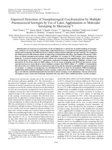
Figure 4: Images of the detected AR orders under (a) complex-valued and (b) magnitudeonly data approaches for the finger-tapping dataset, using the LRT statistic with FDR thresholding at a q ∗ = 0.05 level. 5. Application to fMRI dataset We detected activated voxels for the finger-tapping dataset under both the complex-valued and magnitude-only models. We used the model matrix X described in Section 4 in this application. Our computation of functional activation had three steps: order detection, computation of LRT activation statistics, and thresholding. First, we detected the AR order for each voxel time series, applying the magnitude-only and complex-valued model procedures presented in Section 3.2. As shown in Figure 4, inside the brain, the complex-valued model primarily detected an order of four while the magnitude-only model mostly detected zero or two. Based on these detected orders, LRT activation statistics for the test of H0 : β2 = 0 vs. Ha : β2 6= 0 were calculated for both models. The voxel-wise p-values, computed from the χ21 null distribution, were thresholded at a q ∗ = 0.05 FDR level, determining whether each voxel was detected. The resulting activation maps for complex-valued and magnitude-only statistics are shown in Figures 5(b) and 5(c), respectively. On them, only detected activated voxels are colored – with intensities according the size of the activation statistic – and are overlayed on top of the greyscale anatomical image. Thus, our displayed activation maps display both the location of voxels detected and their “degree” of activation, where larger activation statistics demonstrate stronger activation.

52

JSM2015 - Section on Statistics in Imaging

(a) Anatomical Image

(b) Complex-valued model

(c) Magnitude-only model

Figure 5: (a) Anatomical image of the subject’s brain displaying the central sulci (in green), which contain the sensori-motor finger area cortices. Activation maps of the (b) complexvalued and (c) magnitude-only model LRT statistics (overlayed on top of the same anatomical image), thresholded at the 5% false discovery rate. (Note that activation maps are drawn after masking out voxels outside the brain, as determined by the anatomical image.) We now discuss our findings and the relative advantages of using the complex-valued model over magnitude-only analysis. As indicated earlier, the finger-tapping task has wellestablished fMRI-detected activation regions in the central sulci, which are identified on the anatomical image in Figure 5(a). We argue that the complex-valued model activation map of Figure 5(b) is visually preferable to its magnitude-only counterpart displayed in Figure 5(c). Although both activation maps detect regions of voxels containing the central sulci, the one obtained using the complex-valued model identifies the central sulci more clearly. Also, voxels detected outside the central sulci in the complex map, better adhere to grey matter (shown lighter in Figure 5(a)), which is intrinsically where neural activation takes place. Our maps may also be compared to those in Figure 6 of Rowe and Logan (2004), which are computed (for the same dataset) under the assumption of temporal independence. Our maps, under both complex-valued and magnitude-only models, identify the central sulci more clearly, which we attribute to modeling the AR(p) independence. Thus, we see improved detection and localization abilities in using the time series information, which is enhanced when we use the complex-valued observations over the magnitude-only datasets. 6. Discussion In this paper, we have further developed the complex-valued time series analysis of fMRI data for use in fMRI data analysis. As explained here, fMRI datasets are really complexvalued when collected, but most analysis methods routinely discard the phase information, utilizing only the magnitude images in the data analysis. In doing so, current practice has been to assume a Gaussian distribution for the magnitude data, a supposition that is not even approximately correct for low SNR values. This last point is important to note because SNR (being proportional to voxel volume) decreases with increased spatial resolution. In this paper therefore, we have proposed an AR(p) model for complex-valued time series, thus extending the independent model of Rowe and Logan (2004). Under this model framework, we derived an LRT statistic for detecting activated brain voxels. We compared its performance to a statistic similarly derived under a Gaussian-assumed magnitude-only linear model with AR(p) errors. For low-SNR simulated data, the complex-valued statistic demonstrates notably higher activation detection rates than the Gaussian magnitude-only statistic, due to the inaccuracy of the normal approximation to the Rice-distributed magnitude data. This is potentially advantageous especially for the case of fMRI datasets col-

53

JSM2015 - Section on Statistics in Imaging

lected at higher spatial resolutions and for datasets with higher-level cognitive tasks. In either cases, SNR and CNR values are lower and thus, there is a greater payoff for using the complex-valued approaches. Even for high-SNR simulated data, the complex-valued approach yields lower AR order detection error rates (which negatively affect activation detection) and lower false activation detection rates, simply due to the availability of twice as many quantities in the complex-valued setting. For the finger-tapping dataset, the activation map for the complex-valued statistic more clearly identifies brain regions known to be associated with finger movement – evidence which also indicates a lower false detection rate. There are several aspects of our work that require further attention. For one, we have evaluated and demonstrated performance on a dataset with high SNR in order to establish the validity of our methodology: it would be interesting to also evaluate performance on a low-SNR experimental dataset. There is some scope for optimism here, given the results of our simulation experiments and the fact that our modeling is more accurate than a Gaussian-approximated magnitude-only time series approach which is actually more suspect at lower SNR. Secondly, while we hope that our methods and applications here will spur the adoption of complex-valued methodology for fMRI datasets, we note that since the practice to date has been to rely on magnitude-only fMRI datasets, there are a large number of available datasets for which the phase information has been discarded. For such datasets, temporal models that correctly model the time series in terms of the Rice distribution are needed. It is our view that complex-valued data analysis should become the norm in fMRI: however, for the these datasets, methods on Rice-distributed regression time series that accurately model the temporal correlation also need to be developed. Thus, we note that while we have presented a compelling case for incorporating complex-valued analysis in fMRI, there are many issues that could benefit further with increased attention. References Bandettini, P. A., Jesmanowicz, A., Wong, E. C., and Hyde, J. S. (1993), “Processing strategies for time-course data sets in functional MRI of the human brain,” Magnetic Resonance in Medicine, 30, 161–173. Belliveau, J. W., Kennedy, D. N., McKinstry, R. C., Buchbinder, B. R., Weisskoff, R. M., Cohen, M. S., Vevea, J. M., Brady, T. J., and Rosen, B. R. (1991), “Functional mapping of the human visual cortex by magnetic resonance imaging,” Science, 254, 716–719. Benjamini, Y. and Hochberg, Y. (1995), “Controlling the false discovery rate: a practical and powerful approach to multiple testing,” Journal of the Royal Statistical Society. Series B (Methodology), 57, 289–300. Bullmore, E., Brammer, M., Williams, S. C. R., Rabe-Hesketh, S., Janot, N., David, A., Mellers, J., Howard, R., and Sham, P. (1996), “Statistical methods of estimation and inference for function MR image analysis,” Magnetic Resonance in Medicine, 35, 261– 277. Cochrane, D. and Orcutt, G. (1949), “Applications of least squares regression to relationships containing autocorrelated errors,” Journal of the American Statistical Association, 44, 32–61. den Dekker, A. J., Poot, D. H. J., Bos, R., and Sijbers, J. (2009), “Likelihood-based hypothesis tests for brain activation detection from MRI data disturbed by colored noise: a simulation study,” IEEE Transactions on Medical Imaging, 28, 287–296.

54

JSM2015 - Section on Statistics in Imaging

den Dekker, A. J. and Sijbers, J. (2005), “Implications of the Rician distribution for fMRI generalized likelihood ratio tests,” Magnetic Resonance Imaging, 23, 953–959. Friston, K. J., Frith, C. D., Liddle, P. F., Dolan, R. J., Lammertsma, A. A., and Frackowiak, R. S. J. (1990), “The relationship between global and local changes in PET scans,” Journal of Cerebral Blood Flow and Metabolism, 10, 458–466. Friston, K. J., Holmes, A. P., Worsley, K. J., Poline, J.-B., Frith, C. D., and Frackowiak, R. S. J. (1995), “Statistical parametric maps in functional imaging: A general linear approach,” Human Brain Mapping, 2, 189–210. Friston, K. J., Jezzard, P., and Turner, R. (1994), “Analysis of functional MRI time-series,” Human Brain Mapping, 1, 153–171. Friston, K. J., Josephs, O., Zarahn, E., Holmes, A. P., Rouqette, S., and Poline, J.-B. (2000), “To smooth or not to smooth? Bias and efficiency in fMRI time-series analysis,” NeuroImage, 12, 196–208. Genovese, C. R., Lazar, N. A., and Nichols, T. E. (2002), “Thresholding of statistical maps in functional neuroimaging using the false discovery rate:,” NeuroImage, 15, 870–878. Glover, G. H. (1999), “Deconvolution of impulse response in event-related BOLD fMRI,” NeuroImage, 9, 416–429. Gudbjartsson, H. and Patz, S. (1995), “The Rician distribution of noisy data,” Magnetic Resonance in Medicine, 34, 910–914. Jain, A. K. (1989), Fundaments of Digital Image Processing, Prentice Hall. Jezzard, P. and Clare, S. (2001), “Principles of nuclear magnetic resonance and MRI,” in Functional MRI: An Introduction to Methods, eds. Jezzard, P., Matthews, P. M., and Smith, S. M., Oxford University Press, chap. 3, pp. 67–92. Kwong, K. K., Belliveau, J. W., Chesler, D. A., Goldberg, I. E., Weisskoff, R. M., Poncelet, B. P., Kennedy, D. N., Hoppel, B. E., Cohen, M. S., Turner, R., Cheng, H.-M., Brady, T. J., and Rosen, B. R. (1992), “Dynamic Magnetic Resonance Imaging of Human Brain Activity During Primary Sensory Stimulation,” Proceedings of the National Academy of Sciences of the United States of America, 89, 5675–5679. Lazar, N. A. (2008), The Statistical Analysis of Functional MRI Data, Springer. Locascio, J. J., Jennings, P. J., Moore, C. I., and Corkin, S. (1997), “Time series analysis in the time domain and resampling methods for studies of functional magnetic resonance brain imaging,” Human Brain Mapping, 5, 168–193. Logan, B. R. and Rowe, D. B. (2004), “An evaluation of thresholding techniques in fMRI analysis,” NeuroImage, 22, 95–108. Marchini, J. L. and Ripley, B. D. (2000), “A new statistical approach to detecting significant activation in functional MRI,” NeuroImage, 12, 366–380. Miller, J. W. (1995), “Exact Maximum Likelihood Estimation in Autoregressive Processes,” Journal of Time Series Analysis, 16, 607–615. Nan, F. Y. and Nowak, R. D. (1999), “Generalized Likelihood Ratio Detection for fMRI Using Complex Data,” IEEE Transactions on Medical Imaging, 18, 320–329.

55

JSM2015 - Section on Statistics in Imaging

Ogawa, S., Lee, T. M., Nayak, A. S., and Glynn, P. (1990), “Oxygenation-sensitive contrast in magnetic resonance image of rodent brain at high magnetic fields,” Magnetic Resonance in Medicine, 14, 68–78. Pourahmadi, M. (2001), Foundations of Time Series Analysis and Prediction Theory, Wiley. Purdon, P. L. and Weisskoff, R. M. (1998), “Effect of temporal autocorrelation due to physiological noise and stimulus paradigm on voxel-level false-positive rates in fMRI,” Human Brain Mapping, 6, 239–249. Rice, S. O. (1944), “Mathematical analysis of random noise,” Bell Systems Technical Journal, 23, 282. Rowe, D. B. (2005), “Parameter estimation in the magnitude-only and complex-valued fMRI data models,” NeuroImage, 25, 1124–1132. Rowe, D. B. and Logan, B. R. (2004), “A complex way to compute fMRI activation,” NeuroImage, 23, 1078–1092. — (2005), “Complex fMRI analysis with unrestricted phase is equivalent to a magnitudeonly model,” NeuroImage, 24, 603–606. Shumway, R. H. and Stoffer, D. S. (2006), Time Series Analysis and Its Applications, Springer, second edition ed. Wang, T. and Wei, T. (1994), “Statistical analysis of MR imaging and its applications in image modeling,” Proceedings of the IEEE International Conference on Image Processing and Neural Networks, 1, 866–870. Woolrich, M. W., Ripley, B. D., Brady, M., and Smith, S. M. (2001), “Temporal autocorrelation in univariate linear modeling of FMRI data,” NeuroImage, 14, 1370–1386. Worsley, K. J. and Friston, K. J. (1995), “Analysis of fMRI time-series revisited - again,” NeuroImage, 2, 173–181. Worsley, K. J., Liao, C. H., Aston, J., Petre, V., Duncan, G. H., Morales, F., and Evans, A. C. (2002), “A general statistical analysis for fMRI data,” NeuroImage, 15, 1–15. Worsley, K. J., Marrett, S., Neelin, P., Vandal, A. C., Friston, K. J., and Evans, A. C. (1996), “A unified statistical approach for determining significant voxels in images of cerebral activation,” Human Brain Mapping, 4, 58–73. Zhu, H., Li, Y., Ibrahim, J. G., Shi, X., An, H., Chen, Y., Gao, W., Lin, W., Rowe, D. B., and Peterson, B. S. (2009), “Regression Models for Identifying Noise Sources in Magnetic Resonance Images,” Journal of the American Statistical Association, 104, 623–637.

56