Mar 19, 2014 - some collection such as web pages or photos. ... [3], these are the words ranked highest by LexRank [10], after removal of stop words such ... The Wordle website allows users to ...... [16] K. Koh, B. Lee, B. H. Kim, and J. Seo.
Improved Approximation Algorithms for Box Contact Representations Michael A. Bekos∗
arXiv:1403.4861v1 [cs.DS] 19 Mar 2014
Stephen Kobourov‡
Thomas C. van Dijk† Sergey Pupyrev‡
Martin Fink†
Philipp Kindermann†
Joachim Spoerhase†
Alexander Wolff†
Abstract We study the following geometric representation problem: Given a graph whose vertices correspond to axis-aligned rectangles with fixed dimensions, arrange the rectangles without overlaps in the plane such that two rectangles touch if the graph contains an edge between them. This problem is called Contact Representation of Word Networks (Crown) since it formalizes the geometric problem behind drawing word clouds in which semantically related words are close to each other. Crown is known to be NP-hard, and there are approximation algorithms for certain graph classes for the optimization version, Max-Crown, in which realizing each desired adjacency yields a certain profit. We present the first O(1)-approximation algorithm for the general case, when the input is a complete weighted graph, and for the bipartite case. Since the subgraph of realized adjacencies is necessarily planar, we also consider several planar graph classes (namely stars, trees, outerplanar, and planar graphs), improving upon the known results. For some graph classes, we also describe improvements in the unweighted case, where each adjacency yields the same profit. Finally, we show that the problem is APX-hard on bipartite graphs of bounded maximum degree.
1
Introduction
In the last few years, word clouds have become a standard tool for abstracting, visualizing, and comparing text documents. For example, word clouds were used in 2008 to contrast the speeches of the US presidential candidates Obama and McCain. More recently, the German media used them to visualize the newly signed coalition agreement and to compare it to a similar agreement from 2009 [24]. A word cloud of a given document consists of the most important (or most frequent) words in that document. Each word is printed in a given font and scaled by a factor roughly proportional to its importance (the same is done with the names of towns and cities on geographic maps, for example). The printed words are arranged without overlap and tightly packed into some shape (usually a rectangle). Tag clouds look similar; they consist of keyword metadata (tags) that have been attributed to resources in some collection such as web pages or photos. ∗
Wilhelm-Schickard-Institut f¨ ur Informatik, Universit¨ at T¨ ubingen, Germany. Email: bekos@informatik. uni-tuebingen.de † Lehrstuhl f¨ ur Informatik I, Universit¨ at W¨ urzburg, Germany. http://www1.informatik.uni-wuerzburg. de/en/staff ‡ Department of Computer Science, University of Arizona, USA. http://gama.cs.arizona.edu
1
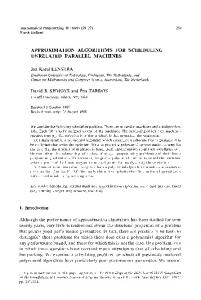
Fig. 1: Semantics-preserving word cloud for the 35 most “important” words in this paper. Following the text processing pipeline of Barth et al. [3], these are the words ranked highest by LexRank [10], after removal of stop words such as “the”. The edge profits are proportional to the relative frequency with which the words occur in the same sentences. The layout algorithm of Barth et al. [3] first extracts a heavy star forest from the weighted input graph as in Theorem 5 and then applies a force-directed post-processing.
Wordle [23] is a popular tool for drawing word or tag clouds. The Wordle website allows users to upload a list of words and, for each word, its relative importance. The user can further select font, color scheme, and decide whether all words must be placed horizontally or whether words can also be placed vertically. The tool then computes a placement of the words, each scaled according to its importance, such that no two words overlap. Generally, the drawings are very compact and aesthetically appealing. In the automated analysis of text one is usually not just interested in the most important words and their frequencies, but also in the connections between these words. For example, if a pair of words often appears together in a sentence, then this is often seen as evidence that this pair of words is linked semantically [17]. In this case, it makes sense to place the two words close to each other in the word cloud that visualizes the given text. This is captured by an input graph G = (V, E) of desired contacts. We are also given, for each vertex v ∈ V , the dimensions (but not the position) of a box Bv , that is, an axis-aligned rectangle. We denote the height and width of Bv by h(Bv ) and w(Bv ), respectively, or, more briefly, by h(v) and w(v). For each edge e = (u, v) of G, we are given a positive number p(e) = p(u, v), that corresponds to the profit of e. For ease of notation, we set p(u, v) = 0 for any non-edge (u, v) ∈ V 2 \ E of G. Given a box B and a point q in the plane, let B(q) be a placement of B with lower left corner q. A representation of G is a map λ : V → R2 such that for any two vertices u 6= v, it holds that Bu (λ(u)) and Bv (λ(v)) are interior-disjoint. Boxes may touch, that is, their boundaries may intersect. If the intersection is non-degenerate, that is, a line segment of positive length, we say that the boxes are in contact. We say that a representation λ realizes an edge (u, v) of G if boxes Bu (λ(u)) and Bv (λ(v)) are in contact. This yields the problem Contact Representation of Word Networks (Crown): Given an edge-weighted graph G whose vertices correspond to boxes, find a representation of G with the vertex boxes such that every edge of G is realized. In this paper, we study the optimization version of Crown, Max-Crown, where the aim is to maximize the total profit (that is, the sum of the weights) of the realized edges. We also consider the unweighted version of the
2
problem, where all desired contacts yield a profit of 1. Previous Work. Barth et al. [2] recently introduced Max-Crown and showed that the problem is strongly NP-hard even for trees and weakly NP-hard even for stars. They presented an exact algorithm for cycles and approximation algorithms for stars, trees, planar graphs, and graphs of constant maximum degree; see the first column of Table 1. Some of their solutions use an approximation algorithm with ratio α = e/(e − 1) ≈ 1.58 [12] for the Generalized Assignment Problem (Gap), defined as follows: Given a set of bins with capacity constraints and a set of items that possibly have different sizes and values for each bin, pack a maximum-valued subset of items into the bins. The problem is APX-hard [6]. Max-Crown is related to finding rectangle representations of graphs, where vertices are represented by axis-aligned rectangles with non-intersecting interiors and edges correspond to rectangles with a common boundary of non-zero length. Every graph that can be represented this way is planar and every triangle in such a graph is a facial triangle. These two conditions are also sufficient to guarantee a rectangle representation [5]. Rectangle representations play an important role in VLSI layout, cartography, and architecture (floor planning). In a recent survey, Felsner [11] reviews many rectangulation variants. Several interesting problems arise when the rectangles in the representation are restricted. Eppstein et al. [9] consider rectangle representations which can realize any given area-requirement on the rectangles, so-called areapreserving rectangular cartograms, which were introduced by Raisz [22] already in the 1930s. Unlike cartograms, in our setting there is no inherent geography, and hence, words can be positioned anywhere. Moreover, each word has fixed dimensions enforced by its importance in the input text, rather than just fixed area. N¨ollenburg et al. [20] recently considered a variant where the edge weights prescribe the length of the desired contacts. Finally, the problem of computing semantics-aware word clouds is related to classic graph layout problems, where the goal is to draw graphs so that vertex labels are readable and Euclidean distances between pairs of vertices are proportional to the underlying graph distance between them. Typically, however, vertices are treated as points and label overlap removal is a post-processing step [8, 14]. Most tag cloud and word cloud tools such as Wordle [23] do not show the semantic relationships between words, but force-directed graph layout heuristics are sometimes used to add such functionality [3, 7, 16, 21, 25]. Our Contribution. Known results and our contributions to Max-Crown are shown in Table 1. Our results rely on two main tools; (i) a PTAS for a special case of Gap [4] and (ii) a lemma for combining results for subgraphs of the given input graph; see Section 2. The combination lemma is quite simple but very useful when a graph can be covered by few subgraphs that belong to graph classes that admit good approximations for Max-Crown. For stars, trees and planar graphs, it suffices to plug the Gap PTAS into the algorithms of Barth et al. [2] to improve their results. Our algorithm for outerplanar graphs, which have not been studied before, also relies on the Gap PTAS. Our other main result is the use of the combination lemma, which, among others, yielded the first approximation algorithms for bipartite and for general graphs; see Section 3. For general graphs, we present a simple randomized solution (based on the solution for bipartite graphs) and a more involved deterministic algorithm. For trees, planar graphs of constant maximum degree, and general graphs, we have improved results in the unweighted case; see Section 4. Finally, we show APX-hardness for bipartite graphs of maximum degree 9 (see
3
Table 1: Previously known and new results for the unweighted and weighted versions of Max-Crown (for α ≈ 1.58 and any ε > 0).
Weighted Graph class
Ratio [2]
cycle, path star tree
1 α 2α NP-hard b(∆ + 1)/2c
max-degree ∆ planar max-deg. ∆ outerplanar planar bipartite
5α
general
Unweighted
Ratio [new]
Ref.
Ratio
Ref.
1+ε 2+ε
Thm. 1 Thm. 1
2
Thm. 6
1+ε
Thm. 7
3+ε 5+ε 16α/3 (≈ 8.4) APX-hard 32α/3 (≈ 16.9; rand.) 40α/3 (≈ 21.1; det.)
Thm. Thm. Thm. Thm. Thm. Thm.
2 1 3 9 4 5
5 + 16α/3 Thm. 8
Section 5) and list some open problems (see Section 6). Model. As in most work on rectangle contact representations, we do not count point contacts of boxes. In other words, we consider two boxes in contact only if their intersection is a line segment of positive length. In this model, the contact graph of the boxes is clearly planar. Our algorithms can easily be modified to guarantee O(1)-approximations also in the model that allows and rewards point contacts; see Appendix B. Runtimes. Most of our algorithms involve approximating a number of Gap instances as a subroutine, using either the PTAS [4] if the number of bins is constant or the approximation algorithm of Fleischer et al. [12] for general instances. Because of this, the runtime of our algorithms consists mostly of approximating Gap instances. Both the PTAS and the existing algorithm solve linear programs, so we refrain from explicitly stating the runtime of these algorithms.
2
Some Basic Results
In this section, we present two technical lemmas that will help us to prove our main results in the following two sections where we treat the weighted and unweighted cases of Max-Crown. The second lemma immediately improves the results of Barth et al. [2] for stars, trees, and planar graphs.
2.1
A Combination Lemma
Several of our algorithms cover the input graph with subgraphs that belong to graph classes for which the Max-Crown problem is known to admit good approximations. The following
4
lemma allows us to combine the solutions for the subgraphs. We say that a graph G = (V, E) is covered by graphs G1 = (V, E1 ), . . . , Gk = (V, Ek ) if E = E1 ∪ · · · ∪ Ek .
Lemma 1. Let graph G = (V, E) be covered by graphs G1 , G2 , . . . , Gk . If, for i = 1, 2, . . . , k, weighted Max-Crown on � graph Gi admits an αi -approximation, then weighted Max-Crown �P k on G admits a i=1 αi -approximation.
Proof. Our algorithm works as follows. For i = 1, . . . , k, we apply the αi -approximation algorithm to Gi and report the result with the largest profit as the result for G. We show that this algorithm has the claimed performance guarantee. For the graphs G, G1 , . . . , Gk , let OPT, OPT1 , . . . , OPTk be the optimum profits and let ALG, ALG1 , . . . , ALGk be the profits of the approximate solutions. By definition, ALGi ≥ OPTi /αi for i = 1, . . . , k. Moreover, P OPT ≤ ki=1 OPTi because the edges of G are covered by the edges of G1 , . . . , Gk . Assume, w.l.o.g., that OPT1 /α1 = maxi (OPTi /αi ). Then Pk OPT1 OPT i=1 OPTi ALG ≥ ALG1 ≥ ≥ P ≥ Pk . k α1 i=1 αi i=1 αi
2.2
Improvement on existing approximation algorithms
Lemma 2 ([4]). For any � > 0, there is a (1 + �)-approximation algorithm for Gap with a constant number of bins. The algorithm takes nO(1/�) time. Using Lemmas 1 and 2, we improve the approximation algorithms of Barth et al. [2]. Theorem 1. Weighted Max-Crown admits a (1 + ε)-approximation algorithm on stars, a (2 + ε)-approximation algorithm on trees, and a (5 + ε)-approximation algorithm on planar graphs. Proof. By Lemma 1, the claim for stars implies the other two claims since a tree can be covered by two star forests and a planar graph can be covered by five star forests in polynomial time [15]. We now show that we can use Lemma 2 to get a PTAS for uc1 uc2 uh2 stars. Here, we give the PTAS for the model with point contacts; in Appendix A we show how to handle the model without point uv1 uv2 u contacts. uh2 Let u be the center vertex of the star. We create eight bins: uc3 uc4 c c c c four corner bins u1 , u2 , u3 , and u4 modeling adjacencies on the four corners of the box u, two horizontal bins uh1 and uh2 modeling ad- Fig. 2: Notation for the jacencies on the top and bottom side of u, and two vertical bins PTAS for stars uv1 and uv2 modeling adjacencies on the left and right side of u; see Fig. 2. The capacity of the corner bins is 1, the capacity of the horizontal bins is the width w(u) of u, and the capacity of the vertical bins is the height h(u) of u. Next, we introduce an item i(v) for any leaf vertex v of the star. The size of i(v) is 1 in any corner bin, w(v) in any horizontal bin, and h(v) in any vertical bin. The profit of i(v) in any bin is the profit p(u, v) of the edge (u, v). Note that any feasible solution to the Max-Crown instance can be normalized so that any box that touches a corner of u has a point contact with u. Hence, the above is an approximation-preserving reduction from weighted Max-Crown on stars (with point contacts) to Gap. By Lemma 2, we obtain a PTAS. 5
3
The Weighted Case
In this section, we consider the weighted Max-Crown problem. First, we give a (3 + ε)approximation for outerplanar graphs. Then, we present a 16α/3-approximation for bipartite graphs. For general graphs, we provide a simple randomized 32α/3-approximation and a deterministic 40α/3-approximation. Theorem 2. Weighted Max-Crown on outerplanar graphs admits a (3 + ε)-approximation. Proof. It is known that the star arboricity of an outerplanar graph is 3, that is, it can be partitioned into at most three star forests [15]. Here we give a simple algorithm for finding such a partitioning. Any outerplanar graph has degeneracy at most 2, that is, it has a vertex of degree at most 2. We prove that any outerplanar graph G can be partitioned into three star forests such that every vertex of G is the center of only one star. Clearly, it is sufficient to prove the claim for maximal outerplanar graphs in which all vertices have degree at least 2. We use induction on the number of vertices of G. The base of the induction corresponds to a 3-cycle for which the claim clearly holds. For the induction step, let v be a degree-2 vertex of G and let (v, u) and (v, w) be its incident edges. The graph G − v is maximal outerplanar and thus, by induction hypothesis, it can be partitioned into star forests F1 , F2 , and F3 such that u is the center of a star in F1 and w is the center of a star in F2 . Now we can cover G with three star forests: we add (v, u) to F1 , we add (v, w) to F2 , and we create a new star centered at v in F3 . Applying Lemmas 1 and 2 to these three star forests completes the proof. Theorem 3. Weighted Max-Crown on bipartite graphs admits a 16α/3-approximation. Proof. Let G = (V, E) be a bipartite input graph with V = V1 ∪˙ V2 and E ⊆ V1 × V2 . Using G, we build an instance of Gap as follows. For each vertex u ∈ V1 , we create eight bins uc1 , uc2 , uc3 , uc4 , uh1 , uh2 , uv1 , uv2 and set the capacities exactly as we did for the star center in Theorem 1. Next, we add an item i(v) for every vertex v ∈ V2 . The size of i(v) is, again, 1 in any corner bin, w(v) in any horizontal bin, and h(v) in any vertical bin. For u ∈ V1 , the profit of i(v) is p(u, v) in any bin of u. It is easy to see that solutions to the Gap instance are equivalent to word cloud solutions (with point contacts) in which the realized edges correspond to a forest of stars with all star centers being vertices of V1 . Hence, we can find an approximate solution of profit ALG01 ≥ OPT01 /α where OPT01 is the profit of an optimum solution (with point contacts) consisting of a star forest with centers in V1 . We now show how to get a solution without point contacts. If the three bins on the top side of a vertex u (two corner bins and one horizontal bin) are not completely full, we can slightly move the boxes in the corners so that point contacts are avoided. Otherwise, we remove the lightest item from one of these bins. We treat the three bottommost bins analogously. Note that in both cases we only remove an item if all three bins are completely full. The resulting solution can be realized without point contacts. We do the same for the three left and three right bins and finally choose the heavier of the two solutions. It is easy to see that we lose at most 1/4 of the profit for the star center u. If we do this for all star centers, we get a solution with profit ALG1 ≥ 3/4 · ALG01 ≥ 3 OPT01 /(4α) ≥ 3 OPT1 /(4α) where OPT1 is the profit of an optimum solution (without point contacts) consisting of a star forest with centers in V1 . 6
H2
H1
G (a) The graph G? realized by an optimum solution is planar and bipartite.
(b) G? can be decomposed into two forests H1 and H2 and further into four star forests S1 , S2 (black) with centers in V1 (disks) and S10 , S20 (dashed) with centers in V2 (boxes).
Fig. 3: Partitioning the optimum solution in the proof of Theorem 3
Similarly, we can find a solution of profit ALG2 ≥ 3 OPT2 /(4α) with star centers in V2 , where OPT2 is the maximum profit that a star forest with centers in V2 can realize. Among the two solutions, we pick the one whose profit ALG = max {ALG1 , ALG2 } is larger. Let G? = (V, E ? ) be the contact graph realized by a fixed optimum solution, and let OPT = p(E ? ) be its total profit. We now show that ALG ≥ 3 OPT /(16α). As G? is a planar bipartite graph, |E ? | ≤ 2n − 4. Hence, we can decompose E ? into two forests H1 and H2 using a result of Nash-Williams [18]; see Fig. 3. We can further decompose H1 into two star forests S1 and S10 in such a way that the star centers of S1 are in V1 and the star centers of S10 are in V2 . Similarly, we decompose H2 into a forest S2 of stars with centers in V1 and a forest S20 of stars with centers in V2 . As we decomposed the optimum solution into four star forests, one of them—say S1 —has profit p(S1 ) ≥ OPT /4. On the other hand, OPT1 ≥ p(S1 ). Summing up, we get ALG ≥ ALG1 ≥ 3 OPT1 /(4α) ≥ 3p(S1 )/(4α) ≥ 3 OPT /(16α). Theorem 4. Weighted Max-Crown on general graphs admits a randomized 32α/3-approximation. Proof. Let G = (V, E) be the input graph and let OPT be the weight of a fixed optimum solution. Our algorithm works as follows. We first randomly partition the set of vertices into V1 and V2 = V \V1 , that is, the probability that a vertex v is included in V1 is 1/2. Now we consider the bipartite graph G0 = (V1 ∪˙ V2 , E 0 ) with E 0 = {(v1 , v2 ) ∈ E | v1 ∈ V1 and v2 ∈ V2 } that is induced by V1 and V2 . By applying Theorem 3 on G0 , we can find a feasible solution for G with weight ALG ≥ 3 OPT0 /(16α), where OPT0 is the weight of an optimum solution for G0 . Any edge of the optimum solution is contained in G0 with probability 1/2. Let OPT be the total weight of the edges of the optimum solution that are present in G0 . Then, E[OPT] = OPT /2. Hence, E[ALG] ≥ 3E[OPT0 ]/(16α) ≥ 3E[OPT]/(16α) = 3 OPT /(32α). Theorem 5. Weighted Max-Crown on general graphs admits a 40α/3-approximation. Proof. Let G = (V, E) be the input graph. As in the proof of Theorem 3, our algorithm constructs an instance of Gap based on G. The difference is that, for every vertex v ∈ V , we create both eight bins and an item i(v). Capacities and sizes remain as before. The profit of placing item i(v) in a bin of vertex u, with u 6= v, is p(u, v). 7
Let OPT be the value of an optimum solution of Max-Crown in G, and let OPTGAP be the value of an optimum solution for the constructed instance of Gap. Since any optimum solution of Max-Crown, being a planar graph, can be decomposed into five star forests [15], there exists a star forest carrying at least OPT /5 of the total profit. Such a star forest corresponds to a solution of Gap for the constructed instance; therefore, OPTGAP ≥ OPT /5. Now we compute an α-approximation for the Gap instance, which results in a solution of total profit ALGGAP ≥ OPTGAP /α ≥ OPT /(5α). Next, we show how our solution induces a feasible solution of Max-Crown where every vertex v ∈ V is either a bin or an item. Consider the directed graph GGAP = (V, EGAP ) with (u, v) ∈ EGAP if and only if the item corresponding to u ∈ V is placed into a bin corresponding to v ∈ V . A connected component in GGAP with n0 vertices has at most n0 edges since every item can be placed into at most one bin. If n0 = 2, we arbitrarily make one of the vertices a bin and the other an item. If n0 > 2, the connected component is a 1-tree, that is, a tree and an edge. In this case, we partition the edges into two subgraphs; a star forest Fig. 4: Partitioning a 1-tree and the disjoint union of a star forest and a cycle; see Fig. 4. into a star forest (gray) and Note that both subgraphs can be represented by touching boxes the union of a cycle and a star forest (black) if we allow point contacts. This is due to the fact that the stars correspond to a solution of GAP. Hence, choosing a subgraph with larger weight and post-processing the solution as in the proof of Theorem 3 results in a feasible solution of Max-Crown with no point contacts. Initially, we discarded at most half of the weight and the post-processing keeps at least 3/4 of the weight, so ALG ≥ 3 ALGGAP /8. Therefore, ALG ≥ 3 OPT /(40α).
4
The Unweighted Case
In this section, we consider the unweighted Max-Crown problem, that is, all desired contacts have profit 1. Thus, we want to maximize the number of edges of the input graph realized by the contact representation. We present approximation algorithms for different graph classes. First, we give a 2-approximation for trees. Then, we present a PTAS for planar graphs of bounded degree. Finally, we provide a (5 + 4α)-approximation for general graphs. Theorem 6. Unweighted Max-Crown on trees admits a 2-approximation. Proof. Let T be the input tree. We first decompose T into edge-disjoint stars as follows. If T has at most two vertices, then the decomposition is straight-forward. So, we assume w.l.o.g. that T has at least three vertices and is rooted at a non-leaf vertex. Let u be a vertex of T such that all its children, say v1 , . . . , vk , are leaf vertices. If u is the root of T , then the decomposition contains only one star centered at u. Otherwise, denote by π the parent of u in T , create a star Su centered at u with edges (u, π), (u, v1 ), . . . , (u, vk ) and call the edge (u, π) of Su the anchor edge of Su . The removal of u, v1 , . . . , vk from T results in a new tree. Therefore, we can recursively apply the same procedure. The result is a decomposition of T into edge-disjoint stars covering all edges of T . We next remove, for each star, its anchor edge from T . We apply the PTAS of Theorem 1 to the resulting star forest and claim that the result is a 2-approximation for T . To prove the claim, consider a star Su0 of the new star forest, centered at u with edges (u, v1 ), . . . , (u, vk ) 8
and let ALG be the total number of contacts realized by the (1 + ε)-approximation algorithm on Su0 . We consider the following two cases. (A) 1 ≤ k ≤ 4: Since it is always possible to realize four contacts of a star, ALG ≥ k. Note that an optimal solution may realize at most k + 1 contacts (due to the absence of the anchor edge from Su0 ). Hence, our algorithm has approximation factor (k + 1)/k ≤ 2. (B) k ≥ 5: Since it is always possible to realize four contacts of a star, we have ALG ≥ 4. On the other hand, an optimal solution realizes at most (1 + ε) ALG +1 contacts. Thus, the approximation factor of our algorithm is ((1+ε) ALG +1)/ ALG ≤ (1+ε)+1/4 < 2. The theorem follows from the fact that all edges of T are incident to the star centers. Next, we develop a PTAS for bounded-degree planar graphs. Our construction needs two lemmas, the first of which was shown by Barth et al. [2]. Lemma 3 ([2]). If the input graph G = (V, E) has maximum degree ∆ then OPT ≥ 2|E|/(∆ + 1). The second lemma provides an exponential-time exact algorithm for Max-Crown. Lemma 4. There is an exact algorithm for unweighted Max-Crown with running time 2O(n log n) . Proof. Consider a placement which assigns a position [`B , rB ]×[bB , tB ] to every box, with `B + w(B) = rB and bB + h(B) = tB . For the x-axis, this gives a (non-strict) linear order on the values `B and rB ; an order on the y-axis is implied similarly. Together, these two orders fully determine the combinatorial structure of overlaps and contacts. (For contact, two boxes must have a side of equal value and a side with overlap, both of which can be seen from the orders.) The algorithm enumerates all possible combinations of these orders. A single order can be enumerated using a permutation of the variables and, between every two variables adjacent in this permutation, whether it is ‘=’ or ‘≤’. The number of orders is bounded by O(22n (2n)!), for a total of 2O(n log n) combinations. For any given pair of orders, it can be determined if they imply overlaps and what the objective value is: the number of profitable contacts. If there are no overlaps, the existence of an actual placement realizing the orders is tested using linear programming. As these tests run in polynomial time, an optimal placement can be found in 2O(n log n) time. Theorem 7. Unweighted Max-Crown on planar graphs with maximum degree ∆ admits a PTAS. More specifically, for any ε > 0 there is an (1 + ε)-approximation algorithm with linear O(1) running time n2(∆/ε) . Proof. Let r be a parameter to be determined later. Frederickson [13] showed that we can √ find a vertex set X ⊆ V (called separator ) of size O(n/ r) such that the following holds. The vertex set V \ X can be partitioned into n/r vertex sets V1 , . . . , Vn/r such that (i) |Vi | ≤ r for i = 1, . . . , n/r and (ii) there is no edge running between any two distinct vertex sets Vi and Vj . In what follows, we assume w.l.o.g. that G is connected, as we can apply the PTAS to every connected component separately. We apply the result of Frederickson to the input graph and compute a separator X. By √ removing the vertex set X from the graph, we remove O(n∆/ r) edges from G. Now, we apply the exact algorithm of Lemma 4 to each of the induced subgraphs G[Vi ] separately. The solution is the union of the optimum solutions to G[Vi ]. 9
Since no edge runs between the distinct sets Vi and Vj , the subgraphs G[Vi ] cover G − X. Let E ? be the set of edges realized by an optimum solution to G, let OPT = |E ? |, and let OPT0 = |E ? ∩ E(G − X)|. By Lemma 3, we have that OPT ≥ 2(n − 1)/(∆ + 1) = √ Ω(n/∆). When we removed X from G, we removed O(n∆/ r) edges. Hence, OPT = √ √ OPT0 +O(n∆/ r) and OPT0 = Ω(n(1/∆ − ∆/ r)). Since we solved each sub-instance G[Vi ] optimally and since these sub-instances cover G − X, the solution created by our algorithm realizes at least OPT0 many edges. Using this fact and the above bounds on OPT and OPT0 , the total performance of our algorithm can be bounded by � � � � √ √ OPT ∆2 OPT0 +O(n∆/ r) n∆/ r √ = 1+O √ . = = 1+O OPT0 OPT0 n(1/∆ − ∆/ r) r−∆ We want this last term to be smaller than 1+ε for some prescribed error parameter 0 < ε ≤ 1. It is not hard to verify that this can be achieved by letting r = Θ(∆4 /ε2 ). Since each of the subgraphs G[Vi ] has at most r vertices, the total running time for determining the solution O(1) is n2(∆/ε) . Before tackling the case of general graphs, we need a lower bound on the size of maximum matchings in planar graphs in terms of the numbers of vertices and edges. Lemma 5. Any planar graph with n vertices and m edges contains a matching of size at least (m − 2n)/3. Proof. Let G be a planar graph. Our proof is by induction on n. The claim clearly holds for n = 1. For the inductive step assume that n > 1. If G is not connected, the claim follows by applying the inductive hypothesis to every connected component. Now assume that G has a vertex u of degree less than 3. Consider the graph G0 = G − u with n0 = n − 1 vertices and m0 ≥ m − 2 edges. By the inductive hypothesis G0 (and hence, G, too) has a matching of size at least (m0 − 2n0 )/3 ≥ ((m − 2) − 2(n − 1))/3 = (m − 2n)/3. It remains to tackle the case where G is connected and has minimum degree 3. Nishizeki and Baybars [19] showed that any connected planar graph with at least n ≥ 10 vertices and minimum degree 3 has a matching of size at least d(n + 2)/3e ≥ n/3. This shows the claim for n ≥ 10 since m ≤ 3n − 6. Finally, we consider the case that G is connected, has minimum degree 3 and n ≤ 9 vertices. First, we assume that a maximum matching of G consists of a single edge e = (u, v). Any edge in G is either equal to or incident on e. Since the minimum degree of G is 3, there is an edge (u, x) 6= e incident on u and an edge (v, y) 6= e incident on v. Since the matching is maximum, we have x = y. Hence, G must be a triangle, which is a contradiction. Now we assume that the maximum matching consists of two edges e = (u, v) and e0 = 0 (u , v 0 ). We show that n ≤ 5, which completes the proof since then 6 ≤ n ≤ 9 guarantees a matching of size at least 3. Assume for a contradiction that there are vertices x and y on which e and e0 are not incident. Due to the maximality of the matching {e, e0 }, edges incident on x and y can only be incident on u, v, u0 , and v 0 . Since x has degree at least 3, G contains, w.l.o.g., the edges (x, u) and (x, v). Since y also has degree 3, y must be adjacent to at least one of the vertices u and v, say u. But then (x, v, u, y) is an augmenting path for the matching, contradicting its optimality.
10
)
V0 V \V 0
)
G0 G¯
¯ (bipartite, gray) (a) G is covered by G and G0 ; perfect matching M (gray, bold).
(b) maximum matching M 00 (gray/black) in G00 = G0 −M .
(c) optimum solution to G0 : graph G∗ (black) and part of M (gray).
Fig. 5: Partitioning the input graph and the optimum solution in the proof of Theorem 8
Theorem 8. Unweighted Max-Crown on general graphs admits a (5+16α/3)-approximation. Proof. The algorithm first computes a maximal matching M in G. Let V 0 be the set of vertices matched by M , let G0 be the subgraph induced by V 0 , and let E 0 be the edge set ¯ = G−E 0 is a bipartite graph with partition (V 0 , V \V 0 ) since the matching of G0 . Note that G M is maximal and hence every edge in E \ E 0 is incident to a vertex of V 0 and to a vertex not ¯ using the algorithm in V 0 ; see Fig. 5a. Hence, we can compute a 16α/3-approximation to G presented in Theorem 3. Consider the graph G00 = (V 0 , E 0 \ M ) and compute a maximum matching M 00 in G00 ; see Fig. 5b. The edge set M ∪ M 00 is a set of vertex-disjoint paths and cycles and can therefore be completely realized [2]. The algorithm realizes this set. Below, we argue that this realization is in fact a 5-approximation for G0 , which completes the proof (due to Lemma 1 and since G ¯ is covered by G0 and G). 0 0 Let n = |V | be the number of vertices of G0 . Let E ∗ be the set of edges realized by an optimum solution to G0 , and let OPT = |E ∗ |. Consider the subgraph G∗ = (V 0 , E ∗ \ M ) of G00 ; see Fig. 5c. Note that G∗ is planar and contains at least OPT −n0 /2 many edges. Applying Lemma 5 to G∗ , we conclude that the maximum matching M 00 of G00 has size at least (OPT −5/2n0 )/3. Hence, by splitting OPT appropriately, we obtain OPT = (OPT −5n0 /2) + 5n0 /2 ≤ 3|M 00 | + 5|M | ≤ 5|M 00 ∪ M | .
5
APX-Hardness
Theorem 9. Weighted Max-Crown is APX-hard even if the input graph is bipartite of maximum degree 9, each edge has profit 1, 2 or 3, and each vertex corresponds to a square of one out of three different sizes. Proof. We give a reduction from 3-dimensional matching (3DM). An instance of this problem is given by three disjoint sets X, Y, Z with cardinalities |X| = |Y | = |Z| = k and a set E ⊆ X × Y × Z of hyperedges. The objective is to find a set M ⊆ E, called matching, such that no element of V = X ∪ Y ∪ Z is contained in more than one hyperedge in M and such that |M | is maximized. The problem is known to be APX-hard [12]. More specifically, for the special case of 3DM where every v ∈ V is contained in at most three hyperedges (hence |E| ≤ 3k) it is NP-hard to decide whether the maximum matching has cardinality k or only k(1 − ε0 ) for some constant 0 < ε0 < 1. We reduce from this special case of 3DM to Max-Crown. To this end, we construct the following Max-Crown instance from a given 3DM instance. We create, for each v ∈ V , a square of side length 1. For each hyperedge e ∈ E, we create 11
e2
e1
e8
e2 x y z e8
e3
e?
e7
e3
e?
e7
e4
e5
e6
e4
e5
e6
(a) profit 7 · 3 + 2 = 23
(b) profit 7 · 3 + 3 · 1 = 24
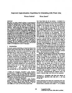
Fig. 6: The two possible configurations of a hyperedge e = (x, y, z) in the proof of Theorem 9
nine squares e? , e1 , . . . , e8 where e? has side length 3.5 and e1 , . . . , e8 have side length 3. In the desired contact graph, we create an edge (e? , e1 ) of profit 2 and, for i = 2, . . . , 8, an edge (e? , ei ) of profit 3. We also create an edge (e? , v) of profit 1 if v is incident to e in the 3DM instance. Consider an optimum solution to the above Max-Crown instance. It is not hard to verify that, for any hyperedge e = (x, y, z), the solution will realize the edges (e? , ei ) for i = 2, . . . , 8. Moreover, we can assume w.l.o.g. that the solution either realizes all three adjacencies (e? , x), (e? , y), and (e? , z) of total profit 3 or the adjacency (e? , e1 ) of profit 2; see Fig. 6 in. We call such a solution well-formed. Assume that there is a solution M to the 3DM instance of cardinality k. Then this can be transformed into a well-formed solution to Max-Crown of profit (7·3+2)|E|+|M | = 23|E|+k. Conversely, suppose that the maximum matching has cardinality at most (1 − ε0 )k. Consider an optimum solution to the respective Max-Crown instance. We may assume that the solution is well-formed. Let M be the set of hyperedges e = (x, y, z) for which all three adjacencies (e? , x), (e? , y), (e? , z) are realized. Then, the profit of this solution is (7 · 3 + 2)|E| + |M | = 23|E| + |M |. Note that M is in fact a matching because the solution to Max-Crown was well-formed. Thus, the optimum profit is bounded by 23|E| + (1 − ε0 )k. Hence, it is NP-hard to distinguish between instances with OPT ≥ 23|E|+k and instances with OPT ≤ 23|E| + (1 − ε0 )k. Using |E| ≤ 3k, this implies that there cannot be any approximation algorithm of ratio less than 23|E| + k ε0 k ε0 k ε0 = 1+ ≥ 1+ = 1+ , 23|E| + (1 − ε0 )k 23|E| + (1 − ε0 )k (70 − ε0 )k 70 − ε0 which is a constant strictly larger than 1.
6
Conclusions and Open Problems
We presented approximation algorithms for the Max-Crown problem, which can be used for constructing semantics-preserving word clouds. Apart from improving approximation factors for various graph classes, many open problems remain. Most of our algorithms are based on covering the input graph by subgraphs and packing solutions for the individual subgraphs. Both subproblems—covering graphs with special types of subgraphs and packing individual solutions together—are interesting problems in their own right. Practical variants of the problem are also of interest, for example, restricting the heights of the boxes to predefined values (determined by font sizes), or defining more than immediate neighbors to be in contact, thus considering non-planar “contact” graphs.
12
References [1] E. Ackerman. A note on 1-planar graphs. Available at http://sci.haifa.ac.il/˜ackerman/ publications/1planar.pdf, Nov. 2013. [p. 15] [2] L. Barth, S. I. Fabrikant, S. Kobourov, A. Lubiw, M. N¨ollenburg, Y. Okamoto, S. Pupyrev, C. Squarcella, T. Ueckerdt, and A. Wolff. Semantic word cloud representations: Hardness and approximation algorithms. In Proc. 11th Latin American Theoret. Inform. Symp. (LATIN’14), volume 8392 of LNCS, pages 514–525. Springer, 2014. Available at arxiv.org/abs/1311.4778. [pp. 3, 4, 5, 9, 11] [3] L. Barth, S. Kobourov, and S. Pupyrev. Experimental comparison of semantic word clouds. In Proc. Symposium on Experimental Algorithms (SEA’14), LNCS. Springer, 2014. To appear. Available at ftp://ftp.cs.arizona.edu/reports/2013/TR13-02.pdf. [pp. 2, 3]
[4] P. Briest, P. Krysta, and B. V¨ ocking. Approximation techniques for utilitarian mechanism design. SIAM J. Comput., 40(6):1587–1622, 2011. [pp. 3, 4, 5] [5] A. L. Buchsbaum, E. R. Gansner, C. M. Procopiuc, and S. Venkatasubramanian. Rectangular layouts and contact graphs. ACM Trans. Algorithms, 4(1), 2008. [p. 3] [6] C. Chekuri and S. Khanna. A PTAS for the multiple knapsack problem. In Proc. 11th ACM-SIAM Symp. Discrete Algorithms (SODA’00), pages 213–222, 2000. [p. 3] [7] W. Cui, Y. Wu, S. Liu, F. Wei, M. Zhou, and H. Qu. Context-preserving dynamic word cloud visualization. IEEE Comput. Graphics Appl., 30(6):42–53, 2010. [p. 3] [8] T. Dwyer, K. Marriott, and P. J. Stuckey. Fast node overlap removal. In Proc. 13th Int. Symp. Graph Drawing (GD’05), volume 3843 of LNCS, pages 153–164. Springer, 2005. [p. 3]
[9] D. Eppstein, E. Mumford, B. Speckmann, and K. Verbeek. Area-universal and constrained rectangular layouts. SIAM J. Comput., 41(3):537–564, 2012. [p. 3] [10] G. Erkan and D. R. Radev. Lexrank: graph-based lexical centrality as salience in text summarization. J. Artif. Int. Res., 22(1):457–479, 2004. [p. 2] [11] S. Felsner. Rectangle and square representations of planar graphs. In J. Pach, editor, Thirty Essays on Geometric Graph Theory, pages 213–248. Springer, 2013. [p. 3] [12] L. Fleischer, M. X. Goemans, V. S. Mirrokni, and M. Sviridenko. Tight approximation algorithms for maximum separable assignment problems. Math. Oper. Res., 36(3):416– 431, 2011. [pp. 3, 4, 11] [13] G. N. Frederickson. Fast algorithms for shortest paths in planar graphs, with applications. SIAM J. Comput., 16(6):1004–1022, 1987. [p. 9] [14] E. R. Gansner and Y. Hu. Efficient, proximity-preserving node overlap removal. J. Graph Algortihms Appl., 14(1):53–74, 2010. [p. 3]
13
[15] S. L. Hakimi, J. Mitchem, and E. F. Schmeichel. Star arboricity of graphs. Discrete Math., 149(1–3):93–98, 1996. [pp. 5, 6, 8] [16] K. Koh, B. Lee, B. H. Kim, and J. Seo. Maniwordle: Providing flexible control over Wordle. IEEE Trans. Vis. Comput. Graph., 16(6):1190–1197, 2010. [p. 3] [17] H. Li and N. Abe. Word clustering and disambiguation based on co-occurrence data. In Proc. 17th Int. Conf. Comput. Linguistics (COLING’98), volume 2, pages 749–755, Stroudsburg, PA, USA, 1998. ACL. [p. 2] [18] C. Nash-Williams. Decomposition of finite graphs into forests. J. London Math. Soc., 39:12, 1964. [p. 7] [19] T. Nishizeki and I. Baybars. Lower bounds on the cardinality of the maximum matchings of planar graphs. Discrete Math., 28(3):255–267, 1979. [p. 10] [20] M. N¨ ollenburg, R. Prutkin, and I. Rutter. Edge-weighted contact representations of planar graphs. In Proc. 20th Int. Symp. Graph Drawing (GD’12), volume 7704 of LNCS, pages 224–235. Springer, 2013. [p. 3] [21] F. V. Paulovich, F. M. B. Toledo, G. P. Telles, R. Minghim, and L. G. Nonato. Semantic wordification of document collections. Comput. Graph. Forum, 31(3):1145–1153, 2012. [p. 3]
[22] E. Raisz. The rectangular statistical cartogram. Geogr. Review, 24(3):292–296, 1934. [p. 3]
[23] F. B. Vi´egas, M. Wattenberg, and J. Feinberg. Participatory visualization with Wordle. IEEE Trans. Vis. Comput. Graphics, 15(6):1137–1144, 2009. [pp. 2, 3] [24] S. Weiland. Der Koalitionsvertrag im Schnellcheck (Quick overview of the [German] coalition agreement). Spiegel Online, www.spiegel.de/politik/deutschland/wasder-koalitionsvertrag-deutschland-bringt-a-935856.html. Click on “Fotos”, 27 Nov. 2013. [p. 1]
[25] Y. Wu, T. Provan, F. Wei, S. Liu, and K.-L. Ma. Semantic-preserving word clouds by seam carving. Comput. Graphics Forum, 30(3):741–750, 2011. [p. 3]
14
Appendix A
The Model without Point Contacts for Stars
We show how we can reduce, for Max-Crown on stars, the case without point contacts to the model with point contacts. This completes the proof of Theorem 1. We first assume that all boxes have integral edge lengths, which can be accomplished by scaling. Consider a feasible solution without point contacts. We now modify the solution as follows. Each box that touches a corner of u is moved so that it has a point contact with this corner. Afterwards, we move some of the remaining boxes until all corners of u have point contacts or until we run out of boxes. This yields a solution with point contacts in which there are two opposite sides of u—say the two horizontal sides—which either do not touch any box or from which we removed one box during the modification. Now observe that, if we shrink the two horizontal sides by an amount of 1/2, then all contacts can be preserved since there was a slack of at least 1 at both horizontal sides. Conversely, observe that any feasible solution with point contacts to the modified instance with shrunken horizontal sides can be transformed into a solution without point contacts since we always have a slack of at least 1/2 on both horizontal sides. This shows that there is a correspondence between feasible solutions without point contacts and feasible solutions with point contacts to a modified instance where we either shrink the horizontal or the vertical sides by 1/2. The PTAS for Max-Crown on stars consists in applying a PTAS to two instances of Max-Crown with point contacts where we shrink the horizontal or vertical sides, respectively, and in outputting the better of the two solutions.
B
The Model with Point Contacts
In the model with point contacts, adjacencies between boxes may be realized by a point contact, that is, if two boxes touch each other in two corners. Note that the APX-hardness proof also holds for this model without any modification. Bipartite and general graphs. For these graph classes, we do, on the one hand, no longer need the post-processing that we applied in Theorems 3 and 5 (and implicitly also in Theorem 4). This post-processing cost us up to a quarter of the total profit. Hence, we can (for now) replace α by 3α/4, which improves the approximation factors for these cases. On the other hand, a realized graph is now not necessarily planar as four boxes can meet in a point and both diagonals correspond to edges of the input graph. It is, however, easy to see that the graphs that can be realized are 1-planar. This means that an optimal solution has at most 4n − 8 edges in the case of general graphs and at most 3n − 6 edges in the case of bipartite graphs. Furthermore, Ackerman [1] showed very recently that a 1-planar graph can be covered by a planar graph and a tree. Hence, we can cover a 1-planar graph with seven star forests and a bipartite 1-planar graph with six star forests (via a bipartite planar graph and a tree). If our approximation algorithm for bipartite graphs uses this decomposition into six star forests, we easily get a 6α-approximation for this case. As a consequence, we get (as in Theorem 4) a randomized 12α-approximation for general graphs. Similarly, decomposing
15
Table 2: Approximation ratios for the version of Max-Crown where point contacts are allowed.
graph class bipartite general
weighted
unweighted
6α 14α (det.), 12α (rand.)
7 + 6α
an optimum 1-planar solution into seven star forests (instead of five star forests for planar graphs), we get a deterministic 14α-approximation for general graphs. Unweighted general graphs. In order to modify the algorithm for the unweighted case, we use the new decomposition of bipartite graphs. It is easy to prove that any 1-planar graph with m edges and n vertices contains a matching of size at least (m − 3n)/3: we planarize the graph (by removing at most n edges) and then apply Lemma 5. This results in a (7 + 6α)-approximation for unweighted general graphs. Table 2 shows the approximation factors for the model with point contacts; in the cases not mentioned in this table, the approximation ratio is the same as in the model without point contacts shown in Table 1.
16