Improved Automatic Detection & Segmentation of Cell

This article has been accepted for publication in a future issue of this journal, but has not been fully edited. Content may change prior to final publication.

TBME-00175-2009.R1

1

Improved Automatic Detection & Segmentation of Cell Nuclei in Histopathology Images Yousef Al-Kofahi, Wiem Lassoued, William Lee, and Badrinath Roysam, Senior Member, IEEE  Abstract— Automatic segmentation of cell nuclei is an essential step in image cytometry and histometry. Despite substantial progress, there is a need to improve accuracy, speed, level of automation, and adaptability to new applications. This paper presents a robust and accurate novel method for segmenting cell nuclei using a combination of ideas. The image foreground is extracted automatically using a graph cuts based binarization. Next, nuclear seed points are detected by a novel method combining multi-scale Laplacian of Gaussian filtering constrained by distance map based adaptive scale selection. These points are used to perform an initial segmentation that is refined using a second graph cuts based algorithm incorporating the method of alpha expansions and graph coloring to reduce computational complexity. Nuclear segmentation results were manually validated over 25 representative images (15 in vitro images and 10 in vivo images, containing more than 7,400 nuclei) drawn from diverse cancer histopathology studies, and four types of segmentation errors were investigated. The overall accuracy of the proposed segmentation algorithm exceeded 86%. The accuracy was found to exceed 94% when only over- and undersegmentation errors were considered. The confounding image characteristics that led to most detection/segmentation errors were high cell density, high degree of clustering, poor image contrast and noisy background, damaged/irregular nuclei, and poor edge information. We present an efficient semi-automated approach to editing automated segmentation results that requires two mouse clicks per operation. Index Terms— Image cytometry, segmentation, cell nuclei, histopathology

T

I. INTRODUCTION

HE goal of this work is to develop efficient and accurate algorithms for detecting and segmenting cell nuclei in two-dimensional (2-D) histological images. This is commonly a first step to counting cells, quantifying molecular Manuscript received February 18, 2009. This work was primarily supported by IDEA grant W81XWH-07-1-0325 BC061142 from the U.S. Army Breast Cancer Research Program. Some aspects were supported by grant R01 EB005157 from the NIBIB, and by NSF grant EEC-9986821 to the Center for Subsurface Sensing & Imaging Systems. Yousef Al-Kofahi is with Rensselaer Polytechnic Institute, Troy, New York 12180 USA (e-mail: [email protected]) Wiem Lassoued is with the University of Pennsylvania, Philadelphia, PA 19104, USA (e-mail: [email protected]) William Lee is with the University of Pennsylvania, Philadelphia, PA 19104, USA (e-mail: [email protected]) Badrinath Roysam is with Rensselaer Polytechnic Institute, JEC 7010, 110 8th Street, Troy, New York 12180 USA (e-mail: [email protected])

markers (antigens) of interest in healthy and pathologic specimens [1, 2], and also for quantifying aspects of normal/diseased tissue architecture [1]. The cell nuclei may be stained using fluorescent markers (e.g., DAPI), or with histochemical stains (e.g., hematoxylin). It is important in these applications to be able to detect the correct number of cells with high accuracy, and to delineate them accurately with utmost automation and minimal human effort. It is also helpful to be able to easily adapt the software algorithms to images of different tissues captured under differing imaging conditions. Automated segmentation of cell nuclei is now a wellstudied topic for which a large number of algorithms have been described in the literature [2-18], and newer methods continue to be investigated. The main challenges in segmenting nuclei in histological, especially pathological tissue specimens, result from the fact that the specimen is a 2D section of a three-dimensional (3-D) tissue sample. The 2-D sectioning can result in partially imaged nuclei, sectioning of nuclei at odd angles, and damage due to the sectioning process. Furthermore, sections have finite thickness resulting in overlapping or partially superposed cells and nuclei in planar images. The end result of these limitations is a set of image objects that differ considerably from the ideal of round blob-like shapes. Their sizes and shapes in images can be irregular, and not always indicative of their 3-D reality. There is natural variability among nuclear shapes and sizes even when they are ideally sectioned. With pathological samples, nuclei can exhibit unnatural shapes and sizes. Variable chromatin texture is another source of segmentation error – highly textured nuclei are harder to segment, especially when they are densely clustered. Separation of densely clustered cell nuclei is a long-standing problem in this field. The presence of a large number of nuclei in the field (especially whole-slide images) necessitates methods that are computationally tractable, in addition to being effective. Finally, imaging noise in the background regions, especially for fluorescence data, and the presence of spectral unmixing errors in processed multispectral images results in additional errors. Perhaps the most critical aspect of nuclear segmentation algorithms is the process of detecting a set of points in the image, usually one per cell nucleus and close to its center, that are variously referred to as “markers” or “seeds”. These points are used by subsequent algorithms to delineate the spatial extent of each cell nucleus. Indeed, the accuracy of the segmentation depends critically on the accuracy and reliability of the initial seed points. Several approaches have been used to detect seed points. The early work in this field [3, 19] relied

Copyright (c) 2009 IEEE. Personal use is permitted. For any other purposes, Permission must be obtained from the IEEE by emailing [email protected]. Authorized licensed use limited to: Rensselaer Polytechnic Institute. Downloaded on November 12, 2009 at 20:10 from IEEE Xplore. Restrictions apply.


TBME-00175-2009.R1 upon the peaks of the Euclidean distance map. This method is often used in conjunction with the watershed algorithm [9] due to its computational efficiency and ready availability. However, it has the widely acknowledged disadvantage of detecting too many seeds, leading to over-segmentation. Some efforts at addressing this limitation include filtering of seeds based on mutual proximity [3], incorporation of additional cues such as the image intensity gradient [9], and the use of region merging algorithms as a post-processing step [10, 11]. Another technique is to detect local maxima points in the gray-scale image using the h-maxima transform [16, 20]. This method was found to be overly sensitive to image texture, and resulted in over-seeding with our images. The Hough transform [21] has also been used for detecting seed points [2, 6]. This method is practical for nearly circular nuclei, and requires excessive computation. More recently, the very elegant iterative radial voting algorithm was presented in [22], and has been used in several papers [14, 23]. This method requires edge extraction based on gradient thresholding, and a careful choice of several parameters that proved impractical in the automated pathology context. In [24] a regularized centroid transform was used. This method only uses the binarized image and does not exploit additional cues present in the image intensity data. In [8], a gradient flow tracking algorithm was used. Like the radial voting idea, this method is conceptually elegant. The difficulty with this method in our experiments was the rough chromatin texture that produces inaccurate flow values and/or directions. In this paper, we present a method that overcomes many of the limitations of the afore-mentioned methods. It is based on the multi-scale Laplacian of Gaussian (LoG) filter originally introduced by Lindeberg [25] as a generic blob detection method. Recently, Byun et al. [4], used a blob detector based on the Laplacian of Gaussian (LoG) filter at a fixed scale (set empirically) to count cells in retinal images. This method offers important advantages, including computational efficiency, ability to exploit shape and intensity information, ease of implementation, especially the ability to specify the approximate expected sizes of nuclei, and robustness to variations. Building upon this work, and keeping in mind the challenges specific to histopathology images noted above, we propose a method combining the Laplacian of Gaussian filter with automatic and adaptive scale selection. Aside from advances in seed detection, the field of automated image analysis has also witnessed the emergence of a new generation of image segmentation algorithms. Notable among these advances are methods based on graph cuts [2630] that offer the important advantage of computing globally optimal solutions. Additional advances have been reported across the literature. Notwithstanding these advances, several needs have remained. For instance, the graph cuts algorithm requires effective initialization. For this, we present a method in which the results of seed detection are processed by a new generation of fast clustering algorithms to generate an initial segmentation that is subsequently refined using the graph-cuts segmentation algorithm. Another important need is to be able to segment large connected clusters of nuclei efficiently and accurately. For this, we introduce a novel segmentation algorithm based on automatic graph coloring and the method of α- expansions. Overall, the effectiveness of the combination

2 of these methods is demonstrated on breast histopathology images. Figure 1 shows a flow-chart illustrating the main steps of our method.

Figure 1: Flow chart outlining the main steps of the proposed nuclear segmentation algorithm. The initial segmentation and refinement steps are illustrated in Figure 2. The optional editing step is illustrated in Figure 3.

II. MATERIALS AND METHODS A. Histology and nuclear staining For the in-vivo tissue examples, de-paraffinized 5 M sections of formalin-fixed, paraffin-embedded human breast tissues were rehydrated, and stained with hematoxylin (Vector Laboratories, Burlingame, CA). For the in-vitro tissue examples, 6 M sections of OCT frozen blocks of cultured K1735 tumor cells were stained with DAPI, 4’,6’-diamidino2-phenylindole (Vector Laboratories, Burlingame, CA). B. Image capture Images of hematoxylin or DAPI stained histopathology slides were captured using a Nuance® multispectral camera (CRI Inc., Woburn, MA) mounted on a Leica epifluorescence microscope (Leica DMRA2). Images were captured using full resolution of the Nuance camera at 8 bits of data per pixel and with 10nm spectral widths from 420 nm to 720 nm for brightfield images, and 440-480 nm for DAPI. Nuance software was used to unmix the chromogens and fluorophores in the data cube into a set of non-overlapping channels based on user–provided reference spectra of the pure chromogens or fluorochromes, respectively. We denote the raw spectral datacube collected by the instrument I ( x, y ,  ) , where

( x, y ) are spatial coordinates of a pixel, and  is the wavelength. The spectral unmixing procedure results in multiple non-overlapping channels that are denoted as follows. The nuclear channel is denoted I N ( x, y ) . This paper is primarily concerned with the processing of

I N ( x, y ) .

C. Automatic Image Binarization The first step in nuclear segmentation is to separate the foreground pixels in the nuclear channel I N ( x, y ) from the background pixels. Several approaches have been presented in the literature, and a survey on image thresholding methods can



TBME-00175-2009.R1

3

be found in [31]. Common methods include histogram-based [32], clustering-based [33-35], and entropy-based [7] algorithms. More advanced techniques are based on graph cuts [15] and level set [36] algorithms, but they require good initialization/training. With this in mind, we propose a hybrid approach that starts with an initial binarization that is subsequently refined using the graph cuts algorithm. For the initial binarization, we compute the normalized image histogram, denoted h(i ) , where i denotes the intensity of a pixel in the range {0...I max } . We found that 128 bins were adequate for these histograms. For the specimens studied here, the histograms were found to be bi-modal as expected, and are modeled well by a mixture of two Poisson distributions. This modeling choice was supported by analysis of the image formation process [37], prior literature [38], and empirical comparison against the more commonly used mixture of Gaussians model [34, 39, 40]. We used the Poisson distribution-based minimum error thresholding algorithm [39, 40]. The normalized image histogram for the mixture of Poisson distributions is written as: (1) h(i )  P0  p (i | 0)  P1  p (i |1) , where P0 and P1 are the a priori probabilities of the

p(i | j ), j  0,1 are Poisson distributions with means  j . For a threshold t , background and foreground regions, and

the Poisson mixture parameters are given by: t

P0 (t )   h(i) i 0

,  0 (t ) 

P1 (t )  1 ( t ) 

t 1 i  h (i ) ;  P0 (t ) i  0

I max

 h(i) ,

i t 1

1 I max  i  h (i ) , P1 (t ) i  t 1

The optimal threshold criterion[39], as follows:

(2)

t  is chosen to minimize an error

t *  arg min   P0 (t )  ln P0 (t )  0 (t ) ln 0 (t )  t

 P1 (t )  ln P1 (t )  1 (t ) ln 1 (t ) 

,

(3)

where  is the mean intensity of the complete image. The result of thresholding

I N ( x, y ) using t  is refined by

incorporating spatial continuity constraints. We seek the pixel labeling L( x, y) that minimizes the following energy function:

E  L ( x, y )  

 D  L( x, y); I

N

( x, y ) 

( x, y )







V  L( x, y ), L( x ', y ') 

,

(4)

( x , y ) ( x ', y ')N ( x , y )

where N ( x, y ) is a spatial neighbor of pixel ( x, y ) . The globally-optimal labeling is computed using the widely-used graph cuts algorithm [26-30, 41, 42]. The first term in equation (4) is the data term representing the cost of assigning

a label to a pixel. It has two-possible values depending upon whether the foreground or background model is used. Mathematically, this is written as follows: D( L( x, y); I N ( x, y))   ln p( I N ( x, y) | j  {0,1}) . (5) The second term is the pixel continuity term that penalizes different labels for neighbouring pixels. Following [26], this is written as follows:

V ( L( x, y ), L( x, y))   ( L( x, y ), L( x, y))



 exp  

I

N



( x, y )  I N ( x, y)  , (6) 2 L2

 

where

 1,  0,

(L(x, y), L( x, y  ))  

if L(x, y)  L( x , y  ); if L(x, y)  L( x , y  ).

. The V-term penalizes different labels for neighbouring pixels when | I N ( x, y )  I N ( x ', y ') |   L . In our work, the scale factor

 L is set empirically to values in the range 20 – 30

pixels. Lower values are used when the image is smooth, and higher values are used when the nuclear chromatin is highly textured. We used an implementation of the fast maxflow/min-cut algorithm described by Boykov et al. [27]. The above method results in accurate binarization results. Figure 2(B) provides a visual example of the binarization results for the image in Figure 2(A). D. Automatic Seed Detection & Initial Segmentation The graph-cuts binarization algorithm extracts connected clusters of nuclei that must be separated into individual nuclei. This requires identification of initial markers (a.k.a. seed points) such that there is one marker per cell. For the present work, multi-scale LoG filter based approaches proved to be the most effective. The Laplacian of Gaussian filter is given by:

 2G( x, y; )  2G( x, y; ) LoG( x, y; )   , (7) x 2 y 2 where  is the scale value, and G ( x, y;  ) is a Gaussian

with 0 mean and scale  . When applied to an image containing blob-like objects, this filter produces a scaleselective peak response at the center of each object with radius r when r   2 . The main advantage of this filter is that the locations of these peaks are robust to the chromatin texture that has a much smaller scale value compared to the nuclear blobs. The filtering results form a topographic surface that provides a basis for cell segmentation. In addition, as we describe below, it provides additional useful information about the boundaries of touching nuclei. A direct application of the multi-scale LoG to images of nuclei would be naïve, since our tissue specimens contain a heterogeneous population of cell types with different nuclear sizes. For this, we propose a multi-scale LoG with automatic scale selection, as described by Lindeberg [25]. While this multi-scale method greatly improved upon the fixed-scale method, as expected, it was nevertheless inadequate as illustrated in Figures 2(C,D). In



TBME-00175-2009.R1 particular, this method fails over heterogeneous clusters of nuclei with different sizes, and weak separating edges. In these cases, it is possible for clusters of 2 or more small nuclei to be detected falsely as a single larger blob that may also encroach on smaller blobs in its vicinity. Overcoming this issue requires a more sophisticated control over the scale values. Our method to achieve such control relies on exploiting shape and size cues available in the Euclidean distance map DN ( x, y ) of the binarized image [43, 44]. Our method proceeds as follows. We compute the response of the scale-normalized LoG filter LoGnorm ( x , y ;  )   2 LoG ( x , y ;  ) at multiple scales

  [ min ,..,  max ] in steps of 1. Then, we use the Euclidean distance map to constrain the maximum scale values when combining the LoG filtering results across scales to compute a single response surface denoted RN ( x, y ) as follows:

RN ( x, y)  arg max  LoGnorm ( x, y;  )  I N ( x, y ) , (8)  [ min , MAX ]

where

 MAX  max  min , min{ max , 2  DN ( x, y )} .

In effect, the distance map constrains the maximum scale value at each point. The response RN ( x, y ) can be thought of as a topographical surface whose peaks indicate centers of individual nuclei – these are the seed points (nuclear markers). We identify the local maxima of RN ( x, y ) , and impose a minimum size (based on the expected range of nuclear diameters) to filter out irrelevant minima, as described further in the following subsection. The effect of using the distance map constraint is illustrated in Figure 2. For instance, panels (C) and (D) show a surface plot of the multi-scale Laplacian of Gaussian and the corresponding initial segmentation (discussed below) respectively. Clearly, the central nucleus is over-smoothed and encroaches into its neighbors. The reason for the encroachment is the use of large  max that is needed to detect large cells in other regions in the image. Figures 2 (E) and (F) respectively show surface plots of RN ( x, y ) and the corresponding initial segmentation. It is clear that the accuracy of seed locations and the initial cells boundaries are much improved by imposing the scale constraint. Using RN ( x, y ) and the seed points detected as described above, we compute an initial segmentation of the nuclei, as described below. The classical approach used by several authors (including ourselves) is based on the watershed algorithm, and its many variants and improvements [2, 3, 5, 911, 16, 45, 46]. This method has the advantage of speed, simplicity, absence of adjustable parameters and a degree of flexibility that results from being able to modify the underlying distance map. The main disadvantage of this algorithm for the present task is its sensitivity to even minor

4 peaks in the distance map that results in over segmentation, and detection of tiny regions as objects. To address this problem, we propose an alternate method based on sizeconstrained clustering. The use of clustering for nuclear/cell segmentation is not new, and predates the watershed method e.g., [45, 47]. However, clustering methods have been computationally expensive and difficult to scale to large images. Recently, Wu et al. [48] described the local-maximum clustering algorithm [48] that overcomes the previous limitations, and paved the way for the present work. This algorithm has a resolution parameter r that is used to define a search area, denoted A( x, y ) of size 2 r  2 r around each pixel in RN ( x, y ) . In a nutshell, this algorithm uses the seed points as cluster centers, and assigns each pixel in the foreground image to these centers to form clusters. To illustrate the effect of varying the resolution parameter on the clustering (initial segmentation results), figure 3 shows two 1-D examples. The shown curve consists of several 1-D blobs with different sizes. When using a small resolution parameter ( r  3 ) all the 3 blobs are detected. The local maxima (seed points) are indicated in dark red, and the vertical dashed-red lines separate the blobs. The direction and length of the black arrows indicate the assignment of each point to its local maximum in a region (distance in 1-D) defined by the resolution parameter. In panel B, we use a larger value of the resolution parameter ( r  6 ). Therefore, the small blob (center) is bypassed and pixels to its left are assigned to their local maxima points to its right. Only two blobs (with two corresponding seed points) were detected. Notice that the separating lines pass through the minima between the two blobs. These points can be thought of as inflection points, where one inflection point is present between blobs. In 2-D images, we have separating boundaries between 2-D blobs. There are two major advantages of using this method over the watershed method [49]. First, the resolution parameter r provides the ability to avoid forming small clusters, as was clearly shown in the two synthetic examples of Figure 3. Second, the clustering method works on foreground points only, which makes it faster. In our experiments, this algorithm was comparably fast to the watershed, and often faster. In our work, the parameter r was set empirically in the range of 5 pixels. Intuitively, r specifies the smallest size of the clusters that we are willing to accept for the next stage of processing. E. Refinement of Initial Nuclear Segmentation using  expansions & Graph Coloring The segmentation contours produced by the above-described cluster analysis are approximate because the clusters are formed using RN ( x, y) rather than the original image, and therefore require further refinement using the image intensity.



TBME-00175-2009.R1

5

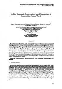
Figure 2: Illustrating key steps of the proposed nuclear segmentation method. (A) Nuclear channel from spectral unmixing. (B) Foreground extraction results. Pixels marked yellow represent a large connected component. (C) Surface plot of the multi-scale LoG filtering results for a small region. (D) Initial segmentation based on the LoG. (E) Surface plot of the distance map constrained multi-scale LoG. (F) Improved initial segmentation resulting from the distance constrained LoG. (G) Color coding of the yellow pixels in panel B. (H) Final segmentation of the image in panel A. Panels (I & J), (K & L), (M & N), (O & P), (Q & R), and (S & T) indicate initial and final segmentation close-ups taken from different regions in the image shown in panel H.

Figure 3: Illustrating the local-maximum clustering method. A 1-D curve with 3 blobs is used. The blob in the middle is very small compared to the others. Two values for the resolution parameter are used. Using in panel (A) results in detecting all 3 blobs. In panel (B), the use of resulted in missing the small blob and merging it to the larger one on the right. The black arrows indicate the assignments of points to their local maxima. The detected seed points are displayed as red dots.

The purpose of the refinement is to enhance the initial contours between touching nuclei to better delineate the true edges between them. To meet this goal, three requirements are needed in the segmentation refinement step. First, it should preserve the shape of the cell nucleus based on some shape model. Second, there should be some rules that prevent two or more nuclei from being merged. This happens if we allow two non-neighbor nuclei to encroach into a third one between them until they merge. Third, given the large number of cell nuclei found in real images, the refinement step should allow multiple cell nuclei need to be refined concurrently for efficiency.



TBME-00175-2009.R1

6

As with the binarization refinement, this step is also formulated as an energy minimization that is solved using a graph-cuts algorithm. However, the problem here is more challenging since we have multiple labels, where the number of labels equals the number of cells in a connected component. In the binary case, the graph cuts method finds the global minima in polynomial time. However, finding a multi-way cut, such that the resulting labeling configuration minimizes the energy function is known to be NP-hard. Boykov et al. [29] introduced two algorithms, known as   expansion and    swap , respectively, that can efficiently find good approximate solutions to the multi-way cut to within a known factor of the global minimum. In this work, the former is used.   expansion method, we formulate the In the segmentation as an iterative binary labeling problem. At each iteration, one label is set to an integer  , and the rest of the labels are set to another value, denoted  , where    . Then, a binary graph-cuts step (called an expansion) is carried out, in which pixel labels are allowed to change in one direction from  to  . The border of the cell labelled with  is refined by expanding it into its neighbours until the energy function is minimized. In the ideal case, the energy function will reach its minimum when the segmentation contour delineates the true nucleus contour, at which the gradient is maximum. The data and smoothness terms of the energy function should be chosen carefully in order to achieve that goal. For the   expansion method to work, the

V has to be a metric, that requires three conditions to hold [29]. Given any three pixel labels L1 , smoothness term denoted

L2 , and L3 , the three conditions are listed below: (1) V ( L1 , L2 )  0



L1  L2 ;

(2) V ( L1 , L2 )  V ( L2 , L1 )  0; (3) V ( L1 , L2 )  V ( L1 , L3 )  V ( L3 , L2 ). We used a spatially varying smoothness function similar to the one used in the binarization step:

V  L ( x, y ), L ( x, y )    ( L ( x, y ), L ( x, y ))

 exp   I N ( x, y )  I N ( x, y )  where:

 Const,  0,

(L(x, y), L( x, y ))  

if L(x, y)  L( x, y ); if L(x, y)  L( x, y ).

The above smoothness function is reached when the labeling discontinuities occur at the edges between the nuclei. The data term at each pixel depends on the likelihood of assigning it to each label (nucleus). As mentioned earlier, the LoG output profile of each nucleus is roughly similar to a Gaussian. In addition, the elliptical shape of the cell is similar to that of the 2-D Gaussian. Hence, a Gaussian model is used to represent each cell. A Maximum Likelihood method (MLE) is used to estimate the Gaussian parameters. The inputs to the MLE are the ( x, y ) coordinates of the pixels of each

nucleus, weighted by the pixel-wise LoG responses. The likelihood for a pixel ( x, y ) to be assigned to cell i is

G ( x, y; i , i ) , where i and i are the mean and the th

covariance matrix of the i Gaussian, respectively. Unfortunately, the   expansion method is not practical when the number of cells in a connected component is large (>20), leading to an excessive number of expansions that require an impractical amount of computer memory and time. To address this difficulty, we propose a novel method based on graph coloring that is described next. We start by noting that when the   expansion procedure is applied to an initially segmented cell, it will only expand to its neighboring regions. This is because the expansion procedure will not assign a pixel to a distant cell. So, we turn the problem into using a small number of labels, with each having a large number of cells expanding in parallel. This is achieved by using a graph coloring approach similar to the one used in [13], but we differ in the use a two-level region adjacency graph. Using the initial segmentation, we build a region adjacency graph. Unlike our prior work [10, 11], we now use a two-level adjacency graph in which a cell is adjacent to its direct neighbors, and to the neighbors’ neighbors as well. The second level of adjacency is added to reduce the possibility that two non-neighboring cells with the same color merge after an expansion. The graph is then colored sequentially such that no two adjacent cells have the same color. Choosing the number of colors is a challenge since the well-known 4-color theorem [50] does not apply in our case because of our twolevel structure. The problem of finding the minimal number of colors is NP-hard. For these reasons, we use a sequential coloring method that is simple to implement, but does not necessarily yield the smallest number of colors. Figure 2(G) shows the coloring output for the initial segmentation of a connected component. That connected component (also shown in yellow in the binarization shown in Figure 2(B)) contains 123 nuclei, but only 8 colors are used. The resulting colors are used as labels for the   expansion step. At each iteration, all the nuclei with a given color are assigned the label  , while all others are assigned  . Then,  cells are expanded concurrently into  cells. As a result, just a few (usually less than 10) expansions are needed regardless of the much larger number of cells in a connected cluster. The smoothness term described above is a pixel-level function, since it depends on the local gradient between adjacent pixels, and hence it is not affected by the grouping of cells based on graph coloring. On the other hand, the data term is a function defined on a cell level, since it is based on a Gaussian model of the cell. Therefore, it is modified in order to compute likelihoods to be assigned to groups (colors) rather than individual cells. Suppose that the number of colors assigned to a connected component with N c cells is N r , where N r  N c . The likelihood that a pixel

( x, y ) will be assigned the j th colour is p  L( x, y )  j   max G ( x, y; i , i ) | Ci  j , j  1 , (9)



TBME-00175-2009.R1

7

The corresponding data term that represents the penalty for assigning pixel ( x, y ) to colour j is:

D( L( x, y)  j; I N ( x, y))   ln p( L( x, y)  j ) ,

(10)

The segmentation refinement consists of multiple iterations of   expansion up to a preset maximum number of iterations (usually 3), or until no change in any pixel label will reduce the energy function. Finally, the resulting objects are renumbered to achieve consistency with the numbers of the initial objects. In Figure 2, panels (I & J), (K & L), (M & N), (O & P), (Q & R), and (S & T) respectively represent initial and refined segmentation close-ups taken from different regions in the image shown in panel H of the same figure. F. Efficient Computer-Assisted Editing of Automated Segmentation Results Automatic segmentation algorithms can provide fast and accurate segmentation of nuclei. However, segmentation errors cannot be avoided even when using optimal parameter values. Hence, human interaction might be needed to fix some the segmentation errors in order to obtain the highest level of accuracy. Indeed, human interaction should be made minimal by tuning the segmentation parameters to reduce the number of errors. In addition, the editing method should be made easy and fast. In this work, two types of errors (defined in the next section) can be corrected using manual editing. The first type is over segmentation and is corrected by merging fragments of over-segmented nuclei. The merging is performed on pairs of neighbor objects by clicking on one point inside each one of them. Figure 4(A, E & I) shows close-ups of initial segmentation results. User selected points (using mouse clicks) for pair of objects that need to be merged are shown in yellow. The merging results are shown in Figure 4(B,F & J). The second type of errors that can be corrected is under segmentation. An under-segmented object is split into two objects by clicking at two points inside it. An automatic splitting method is used to draw an initial contour between the two new objects. The splitting method starts by computing the approximate Euclidian distances from each point inside the undersegmented object to the manually selected points. Then, the splitting is done based on the minimum of the two distances at each point. Blue crosses in Figure 4(B,F & J) represent user selected pairs of points indicating objects that need to be split. Figure 4(C,G & K) shows the automatic splitting results. Changes to the initial segmentation caused by editing are also applied on all the images needed in the segmentation refinement step. As illustrated previously, the refinement step uses a Graph-Cuts based technique (   expansion ), where both the initial segmentation and the LoG output ( RN ( x, y ) ) are needed. The editing methods mentioned above will update the labels in the initial segmentation. On the other hand, the LoG output RN ( x, y ) is updated as follows. In the case of over-segmentation, the LoG output profile of the oversegmented object is replaced by the inverted distance map from the center of the new object produced by merging. On the other hand, the LoG output profile of an over-segmented object is replaced by the inverted distance map from the

centers of the two new objects resulting from splitting. Figure 4(D,H & L) show the final segmentation after refinement. A related two-mouse-click based technique for interactive whole cell segmentation was presented in [51], where the user segments one cell at a time by clicking on a point at the center of cell and another one on its border. The image is then transformed into polar coordinates, a dynamic programming algorithm is used to find the optimal path on the cell border from left to right, and finally that path is mapped back into Cartesian coordinates. One drawback of the presented editing tool is the need to scan the image visually to search for segmentation errors. This can be a time consuming task in very large images with large numbers of cells. One possible solution is to adopt the approach presented by the same group [52] in which a segmentation confidence score is computed for each segmented cell nucleus based on some morphological an intensity based features. The lower the confidence score, the more likely the segmentation error is. Then, segmented cell nuclei are sorted based on their confidence scores and the user starts inspecting those them starting from those with low confidence values. Yet another approach that is explored as part of the FARSIGHT project (www.farsight-toolkit.org) is to identify outliers (based on one or more features) to detect nuclei that require further inspection for potential editing. In general, the use of pattern analysis tools to guide the user for expedited editing is a topic of ongoing research. III. RESULTS AND VALIDATION The results of automated analysis for 25 representative images (15 in-vitro images and 10 in-vivo images, containing more than 7,400 nuclei in all) drawn from diverse cancer histopathology studies were inspected and scored manually with the goal of developing a conservative assessment of the frequency and types of segmentation errors. The manual scoring was recorded electronically, and a sample is displayed in Figure 5A. In this figure, the type of error is indicated as a color-coded dot. Seeds of correctly segmented nuclei are displayed as green dots. Under-segmentation errors (i.e., a failure to split a region into the correct number of nuclei) are indicated as dark blue dots. Over-segmentation errors (i.e., excessive splitting) are indicated as purple dots. In addition to these standard types of errors, we also looked for encroachment errors (indicated as yellow dots) that occur when the automated algorithms do not correctly place the boundary between a pair of touching nuclei. In other words, it is the error in delineating the true border between two nuclei. The last type of segmentation errors is binarization errors. This type of error includes the case of nuclei encroaching on their neighbors, or nuclei encroached over by their neighbors. The main difficulty with quantification of encroachment errors is its innate subjectivity. Another difficulty is the acceptance threshold. In a strict sense, one could argue successfully that every adjacent pair of nuclei suffers from some encroachment error. In our work, a slight encroachment of a few pixels that does not change the nucleus shape or size significantly is not considered as an error. We only consider moderate to severe encroachment errors in which the error corresponds to at least 25 percent of the total nucleus area. Although this manual



TBME-00175-2009.R1

8

observation is still subjective and may vary from an observer to another, it can give a good approximation of the number of encroachment errors. Furthermore, we also examined errors from automatic binarization of the image data. The binarization is visualized as boundaries overlaid on the image (Figure 5A). Incorrectly binarized nuclei are indicated with light blue dots in Figure 5A. We considered errors for which a cell nucleus or part of it is missed at the binarization step.

panel D. It is clear that significant improvement is achieved after applying graph-cuts refinement.

Figure 4: Illustrating the impact of (optional) seed editing on the final segmentation. Initial segmentations are shown in the first column (A,E & I) for 3 selected regions. Yellow crosses indicate locations of mouse clicks requesting pairs of segmented objects to be merged. The results of merging are shown in the second column (B,F & J), in addition to the user’s requests to split objects indicated as blue crosses. The blue crosses are initial seeds locations for the two new objects. The results of splitting are shown in the third column (C,G & K). The final segmentation after refinement is shown in the fourth column (D,H & L).

Figure 4: Illustrating the results validation criteria. (A) Segmentation output of an image with color coded seeds on each nucleus to identify whether it is correctly segmented or the type of segmentation error. (B) An example of an under-segmentation error. (C) An example of over-segmentation error. (D) An example of an encroachment error. (E) An example of a binarization error. Table 1: Summary of segmentation performance data for 25 sample images*

Finally, Figure 6 shows six typical examples of segmented nuclear images. All of the scoring results are provided to the reader in the electronic supplement. Table I summarizes the error analysis using 25 images. The first 15 in the table are invitro images while the last 10 are in-vivo. Overall, just considering under- and over-segmentation errors alone, our fully automated algorithm achieved > 94% accuracy. This data is helpful in comparing our algorithm to previously published methods [9, 18]. When encroachment and binarization errors are included, our algorithm showed an accuracy of more than 86%. The performance of our algorithm with regard to over- and under-segmentation errors can be described in terms of precision and recall measures. Specifically, the last two columns of these values are indicated in Table I. The overall F-measure (2  precision  recall)/(precision + recall) for these data is 0.97. We studied the performance of our binarization refinement step by comparing its output with the initial binarization using 20 2-D phantom images for which we have ground truth data. For each image, we compared the percentages of incorrectly labeled pixels before and after binarization refinement using graph cuts as detailed in Table II. Figure 7 (A &B) shows a sample phantom image and the corresponding ground truth. Initial segmentation output is shown in panel C, while the refinement output is shown in



TBME-00175-2009.R1

9

Figure 5: Sample segmentation results of six 2-D nuclear images including two in-vitro images (Panels A & B) and four in-vivo images (Panels C-F).

Finally, we studied the complexity reduction achieved using graph coloring by comparing segmentation processing times with and without graph coloring for 15 automatically created phantom images. All the images have the same size ( 300  300 ), with only one connected component (cluster of nuclei), and a varying number of nuclei in each cluster (10 150). Table III shows a summary of the analysis. Increasing numbers of nuclei in the cluster results in rapidly increasing processing time when graph coloring is not used. That is because the number of required  -expansions is equal to the number of nuclei in the cluster. However, no significant increase in processing time is noticed when graph coloring is

used, since the number of  -expansions is equal to the number of colors, which is in the range of 5 to 10 colors. Three sample phantom images are shown in Figure 8 (A, B, & C) containing 10, 70, and 130 nuclei respectively. The segmentation results are shown as red outlines. A graphical representation of the results in Table III is shown in Figure 8 (D), which shows 2-D plots of the number of cells in the connected component (cluster) versus the processing time for both cases. IV. DISCUSSION The present work has built upon, integrated, and extended multiple recent advances in the biological image analysis field.



TBME-00175-2009.R1 The resulting algorithms have proved to be extremely robust and accurate. In our experience, the usually tricky task of choosing the optimal parameter settings for the proposed algorithm is both simple as well as intuitive. When errors do occur, our method of editing the seeds, followed by segmentation refinement is extremely efficient in practice. It requires minimal effort, and makes best use of the human observer’s ability to discern complex patterns, and resolve ambiguities. The actual segmentation is best carried out computationally.

10 or when the nucleus shape is extremely elongated. This is particularly common with nuclei that deviate significantly from a blob shape, as is the case with some vascular endothelial cells. Under-segmentation usually occurs when nuclei (especially small ones) are highly clustered with weak borders between the nuclei. The causes of encroachment errors were much more diverse, and most often caused by weak object separation cues in the image. The above types of errors are, to some extent, influenced by the choice of parameter settings. This is discussed further below. Binarization errors were largely due to variations in the nuclear signal intensity, specifically, a weak signal resulted in most binarization errors. Table 3: Illustrating the complexity and processing time reduction after using graph coloring

Figure 6: Comparing initial and graph-cut refined binarization results using a phantom image for which the ground truth is known. (A) A 2D phantom image. (B) Binarization ground truth. (C) Initial binarization output. (D) Results of binarization refinement using graph cuts. Table 2: Comparison of binarization accuracy before and after Graph-Cut refinement

Figure 7: Illustrating the effect of graph coloring using 15 phantom images with the same size and one nuclear cluster, but with different number of nuclei (x axis). Three examples are shown in panels A, B & C containing 10, 70, and 130 nuclei respectively. Detected seeds are shown as green dots and nuclear segmentation results are shown as red outlines. Panel D is a plot of the number of cell nuclei in the cluster versus segmentation processing time (without graph coloring in red and with graph coloring in blue).

There are several known sources of the errors analyzed by us. Over-segmentation usually happens when a nucleus’ chromatin is highly textured (especially true for large nuclei)

A traditional difficulty with automated algorithms is the effort required to tune them by selecting appropriate parameter settings to new images and applications. In this regard, the algorithms we described are well behaved and intuitive. The main parameters that must be provided to the software include the minimum scale for the LoG filter  min , the maximum



TBME-00175-2009.R1

11

scale value  max , that define the expected range of sizes of the nuclei. In our experiments, we used values in the range of 4 – 8 pixels for  min , and 10 – 20 pixels for  max . Although our algorithms are multi-scale by design, the choice of these parameters affects the balance of over- and undersegmentation errors to a small extent. Among these two parameters,  min is more influential. Specifically, if the value

of  min is much smaller than the expected minimum size of the nuclei, then the incidence of over-segmentation increases. Smaller values of this parameter are also needed to account for small fragments of nuclei that are characteristic of 2D sections of 3D tissue. On the other hand, if the value of  max is too low, over-segmentation errors become more prevalent. An overly high value of  max is much more benign in nature because it is used in combination with the distance map – it can result in under-segmentation or encroachment errors when exceptionally large and highly clustered groups of nuclei are encountered. The clustering resolution parameter r was generally chosen in the 3 – 5 pixel range, and the weighting parameter  L for the graph cuts segmentation algorithm was in the range of 20 – 30. The algorithm described here is incorporated into the FARSIGHT toolkit [52] that is designed to analyze multiparameter histopathology images. This software system and implementations of the algorithms reported here are available to interested colleagues from the corresponding author.

[8]

[9]

[10]

[11]

[12] [13]

[14]

[15] [16]

[17]

ACKNOWLEDGMENT The authors wish to thank Dr. Sumit Nath for helpful discussions.

[18] [19]

REFERENCES [1]

[2]

[3]

[4]

[5]

[6]

[7]

C. Bilgin, C. Demir, C. Nagi, and B. Yener, “Cell-Graph Mining for Breast Tissue Modeling and Classification,” in Proc. Engineering in Medicine and Biology Society, 2007. EMBS 2007. 29th Annual International Conference of the IEEE, 2007, pp. 5311 - 5314. C. Ortiz de Solorzano, E. Garcia Rodriguez, A. Jones, D. Pinkel, J.W. Gray, D. Sudar, and S.J. Lockett, “Segmentation of confocal microscope images of cell nuclei in thick tissue sections,” J Microsc, vol. 193, (no. Pt 3), pp. 212-26, Mar 1999. H. Ancin, B. Roysam, T.E. Dufresne, M.M. Chestnut, G.M. Ridder, D.H. Szarowski, and J.N. Turner, “Advances in automated 3-D image analyses of cell populations imaged by confocal microscopy,” Cytometry, vol. 25, (no. 3), pp. 221-34, Nov 1 1996. J.Y. Byun, M.R. Verardo, B. Sumengen, G.P. Lewis, B.S. Manjunath, and S.K. Fisher, “Automated tool for the detection of cell nuclei in digital microscopic images: Application to retinal images,” Molecular Vision, vol. 12, (no. 105-07), pp. 949-960, Aug 16 2006. M.K. Chawla, G. Lin, K. Olson, A. Vazdarjanova, S.N. Burke, B.L. McNaughton, P.F. Worley, J.F. Guzowski, B. Roysam, and C.A. Barnes, “3D-catFISH: a system for automated quantitative three-dimensional compartmental analysis of temporal gene transcription activity imaged by fluorescence in situ hybridization,” J Neurosci Methods, vol. 139, (no. 1), pp. 13-24, Oct 15 2004. C.O. De Solorzano, R. Malladi, S.A. Lelievre, and S.J. Lockett, “Segmentation of nuclei and cells using membrane related protein markers,” Journal of Microscopy-Oxford, vol. 201, pp. 404-415, Mar 2001. P.R. Gudla, K. Nandy, J. Collins, K.J. Meaburn, T. Misteli, and S.J. Lockett, “A high-throughput system for segmenting nuclei using multiscale techniques,” Cytometry A, vol. 73, (no. 5), pp. 451-66, May 2008.

[20] [21] [22] [23] [24] [25] [26] [27]

[28] [29]

G. Li, T.M. Liu, J.X. Nie, L. Guo, J. Malicki, A. Mara, S.A. Holley, W.M. Xia, and S.T.C. Wong, “Detection of blob objects in microscopic zebrafish images based on gradient vector diffusion,” Cytometry Part A, vol. 71A, (no. 10), pp. 835-845, Oct 2007. G. Lin, U. Adiga, K. Olson, J.F. Guzowski, C.A. Barnes, and B. Roysam, “A hybrid 3D watershed algorithm incorporating gradient cues and object models for automatic segmentation of nuclei in confocal image stacks,” Cytometry A, vol. 56, (no. 1), pp. 23-36, Nov 2003. G. Lin, M.K. Chawla, K. Olson, C.A. Barnes, J.F. Guzowski, C. Bjornsson, W. Shain, and B. Roysam, “A multi-model approach to simultaneous segmentation and classification of heterogeneous populations of cell nuclei in 3D confocal microscope images,” Cytometry A, vol. 71, (no. 9), pp. 724-36, Sep 2007. G. Lin, M.K. Chawla, K. Olson, J.F. Guzowski, C.A. Barnes, and B. Roysam, “Hierarchical, model-based merging of multiple fragments for improved three-dimensional segmentation of nuclei,” Cytometry A, vol. 63, (no. 1), pp. 20-33, 2005. S.K. Nath, F. Bunyak, and K. Palaniappan, “Robust Tracking of Migrating Cells Using Four-Color Level Set Segmentation,” Lect Notes Comput Sci, vol. 4179, (no. LNCS), pp. 920-932, 2006. S.K. Nath, K. Palaniappan, and F. Bunyak, “Cell segmentation using coupled level sets and graph-vertex coloring,” Medical Image Computing and Computer-Assisted Intervention - Miccai 2006, Pt 1, vol. 4190, pp. 101-108, 2006. B. Parvin, Q. Yang, J. Han, H. Chang, B. Rydberg, and M.H. BarcellosHoff, “Iterative voting for inference of structural saliency and characterization of subcellular events,” Ieee Transactions on Image Processing, vol. 16, (no. 3), pp. 615-623, Mar 2007. C. Russell, D. Metaxas, C. Restif, and P. Torr, “Using the Pn Potts model with learning methods to segment live cell images,” in Proc. IEEE 11th International Conference on Computer Vision, 2007, pp. 1-8. C. Wahlby, I.M. Sintorn, F. Erlandsson, G. Borgefors, and E. Bengtsson, “Combining intensity, edge and shape information for 2D and 3D segmentation of cell nuclei in tissue sections,” Journal of MicroscopyOxford, vol. 215, pp. 67-76, Jul 2004. M. Wang, X. Zhou, F. Li, J. Huckins, R.W. King, and S.T. Wong, “Novel cell segmentation and online SVM for cell cycle phase identification in automated microscopy,” Bioinformatics, vol. 24, (no. 1), pp. 94-101, Jan 1 2008. G. Li, T. Liu, A. Tarokh, J. Nie, L. Guo, A. Mara, S. Holley, and S.T. Wong, “3D cell nuclei segmentation based on gradient flow tracking,” BMC Cell Biol, vol. 8, pp. 40, 2007. N. Malpica, C.O. de Solorzano, J.J. Vaquero, A. Santos, I. Vallcorba, J.M. Garcia-Sagredo, and F. del Pozo, “Applying watershed algorithms to the segmentation of clustered nuclei,” Cytometry, vol. 28, (no. 4), pp. 289-97, Aug 1 1997. P. Soille, Morphological Image Analysis: Principles and Applications: Springer-Verlag Telos 1999. D.H. Ballard, “Generalizing the Hough Transform to Detect Arbitrary Shapes,” Pattern Recognition, vol. 13, (no. 2), pp. 111-122, 1981. Q. Yang and B. Parvin, “Perceptual Organization of Radial Symmetries,” in Proc. IEEE Computer Society Conference on Computer Vision and Pattern Recognition 2004, pp. 320-325. H. Chang, Q. Yang, and B. Parvin, “Segmentation of heterogeneous blob objects through voting and level set formulation,” Pattern Recognition Letters, vol. 28, (no. 13), pp. 1781-1787, Oct 1 2007. Q. Yang and B. Parvin, “Harmonic cut and regularized centroid transform for localization of subcellular structures,” IEEE Transactions on Biomedical Engineering, vol. 50, (no. 4), pp. 469-475, Apr 2003. T. Lindeberg, “Feature detection with automatic scale selection,” International Journal of Computer Vision, vol. 30, (no. 2), pp. 79-116, Nov 1998. Y. Boykov and G. Funka-Lea, “Graph cuts and efficient N-D image segmentation,” International Journal of Computer Vision, vol. 70, (no. 2), pp. 109-131, Nov 2006. Y. Boykov and V. Kolmogorov, “An experimental comparison of mincut/max-flow algorithms for energy minimization in vision,” IEEE Transactions on Pattern Analysis and Machine Intelligence, vol. 26, (no. 9), pp. 1124-1137, Sep 2004. Y. Boykov and J.M. P., “Interactive graph cuts for optimal boundary & region segmentation of objects in N-D images,” in Proc. International Conference on Computer Vision, 2001, pp. 1025-112. Y. Boykov, O. Veksler, and R. Zabih, “Fast approximate energy minimization via graph cuts,” IEEE Transactions on Pattern Analysis and Machine Intelligence, vol. 23, (no. 11), pp. 1222-1239, Nov 2001.



TBME-00175-2009.R1 [30] V. Kolmogorov and R. Zabih, “What energy functions can be minimized via graph cuts?,” IEEE Transactions on Pattern Analysis and Machine Intelligence, vol. 26, (no. 2), pp. 147-159, Feb 2004. [31] M. Sezgin and B. Sankur, “Survey over image thresholding techniques and quantitative performance evaluation,” Journal of Electronic Imaging, vol. 13, (no. 1), pp. 146-168, Jan 2004. [32] R. Guo and S.M. Pandit, “Automatic threshold selection based on histogram modes and a discriminant criterion,” Machine Vision and Applications, vol. 10, (no. 5-6), pp. 331-338, Apr 1998. [33] J. Kittler and J. Illingworth, “On Threshold Selection Using Clustering Criteria,” IEEE Transactions on Systems Man and Cybernetics, vol. 15, (no. 5), pp. 652-655, 1985. [34] J. Kittler and J. Illingworth, “Minimum Error Thresholding,” Pattern Recognition, vol. 19, (no. 1), pp. 41-47, 1986. [35] N. Otsu, “Threshold Selection Method from Gray-Level Histograms,” IEEE Transactions on Systems Man and Cybernetics, vol. 9, (no. 1), pp. 62-66, 1979. [36] J. Lie, M. Lysaker, and X.C. Tai, “A binary level set model and some applications to Mumford-Shah image segmentation,” IEEE Transactions on Image Processing, vol. 15, (no. 5), pp. 1171-1181, May 2006. [38] N.R. Pal and S.K. Pal, “Image model, Poisson distribution and object extraction,” International Journal of Pattern Recognition and Artificial Intelligence, vol. 5, (no. 3), pp. 25, 1991. [39] J.L. Fan, “Notes on Poisson distribution-based minimum error thresholding,” Pattern Recognition Letters, vol. 19, (no. 5-6), pp. 425431, Apr 1998. [40] N.R. Pal and D. Bhandari, “On Object Background Classification,” International Journal of Systems Science, vol. 23, (no. 11), pp. 19031920, Nov 1992. [41] Y. Boykov, O. Veksler, and R. Zabih, “Markov random fields with efficient approximations,” in Proc. IEEE Conference on Computer Vision and Pattern Recognition 1998, pp. 648-655. [42] D. Geiger, A. Gupta, L.A. Costa, and J. Vlontzos, “Dynamic programming for detecting, tracking, and matching deformable contours (vol 17, pg 294 1995),” IEEE Transactions on Pattern Analysis and Machine Intelligence, vol. 18, (no. 5), pp. 575-575, May 1996. [43] G.J. Breu H, Kirkpatrick D, Werman M, “Linear Time Euclidean Distance Transform Algorithms,” IEEE Transactions on Pattern Analysis and Machine Intelligence, vol. 17, (no. 5), pp. 529-533, May 1995. [44] O. Cuisenaire, “Fast Euclidean distance transformations by propagation using multiple neighbourhoods,” Computer Vision and Image Understanding, vol. 76, (no. 2), pp. 163-172, November 1999. [45] R.W. Mackin, B. Roysam, T.J. Holmes, and J.N. Turner, “Automated three-dimensional image analysis of thick and overlapped clusters in cytologic preparations. Application to cytologic smears,” Anal Quant Cytol Histol, vol. 15, (no. 6), pp. 405-17, Dec 1993. [46] R.W. Mackin, Jr., L.M. Newton, J.N. Turner, and B. Roysam, “Advances in high-speed, three-dimensional imaging and automated segmentation algorithms for thick and overlapped clusters in cytologic preparations. Application to cervical smears,” Anal Quant Cytol Histol, vol. 20, (no. 2), pp. 105-21, Apr 1998. [47] B. Roysam, H. Ancin, A.K. Bhattacharjya, M.A. Chisti, R. Seegal, and J.N. Turner, “Algorithms for automated characterization of cell populations in thick specimens from 3-D confocal fluorescence microscopy data,” J Microsc, vol. 173, (no. Pt 2), pp. 115-26, Feb 1994. [48] X.W. Wu, Y.D. Chen, B.R. Brooks, and Y.A. Su, “The local maximum clustering method and its application in microarray gene expression data analysis,” Eurasip Journal on Applied Signal Processing, vol. 2004, (no. 1), pp. 53-63, Jan 1 2004. [49] L. Vincent and P. Soille, “Watersheds in Digital Spaces - an Efficient Algorithm Based on Immersion Simulations,” IEEE Transactions on Pattern Analysis and Machine Intelligence, vol. 13, (no. 6), pp. 583-598, Jun 1991. [50] N. Robertson, D.P. Sanders, P. Seymour, and R. Thomas, “Efficiently four-coloring planar graphs,” in Proc. Proceedings of the twenty-eighth annual ACM symposium on Theory of computing, 1996, pp. 571-575. [51] D. Baggett, M.A. Nakaya, M. McAuliffe, T.P. Yamaguchi, and S. Lockett, “Whole cell segmentation in solid tissue sections,” Cytometry A, vol. 67, (no. 2), pp. 137-43, Oct 2005. [52] C.S. Bjornsson, G. Lin, Y. Al-Kofahi, A. Narayanaswamy, K.L. Smith, W. Shain, and B. Roysam, “Associative image analysis: a method for automated quantification of 3D multi-parameter images of brain tissue,” J Neurosci Methods, vol. 170, (no. 1), pp. 165-78, May 15 2008.

12 Yousef Al-Kofahi received the B.S degree in computer engineering from Yarmouk University, Irbid, Jordan, in 2003, and the M.S. degree from the Electrical, Computer and Systems Engineering (ECSE) Department, Rensselaer Polytechnic Institute (RPI), Troy, NY, in 2005. He is currently a Ph.D. candidate in computer systems engineering at RPI. His current research interest includes computer vision, pattern recognition, and image processing/analysis. His Ph.D. research is focused on developing computer vision and machine learning algorithms for objectlevel mapping of complex biological tissues from 2D/3D multi-spectral images. Wiem Lassoued received her master degree in Sciences from the University of Sciences of Tunis in Tunisia in 2001. She has been working as a specialist researcher C at Dr William’s Lee laboratory for the past 5 years, at the University of Pennsylvania, Abramson Cancer center. In her research, one of her area of interest is to develop computerized quantitative analysis of histopatholgy tumor specimen based on image analysis, and look at different mechanisms involved to develop cancer. William Lee received his Ph.D. and M.D. from the University of Chicago, Chicago, IL in 1974 and 1975, respectively. He is currently an Associate Professor of Medicine in the Division of Hematology-Oncology, co-leader of the Tumor Biology Program in the Abramson Cancer Center, and an Associate Editor of the Journal of Clinical Investigation. A major focus of his research is development of methods for quantitative analysis of human tumor histopathology and of the biological events and processes preserved in these specimens. Badrinath Roysam (SM ’89) received the B. Tech degree in electronics engineering from the Indian Institute of Technology, Madras, India, in 1984, and the M.S. and D.Sc. degrees from Washington University, St. Louis, in 1987, and 1989, respectively. He has been at Rensselaer Polytechnic Institute, Troy, New York since 1989, where he is currently a Professor in the Electrical, Computer and Systems Engineering Department. He is an associate director of the Center for Subsurface Sensing and Imaging Systems (CenSSIS) - a multi-university NSF-sponsored engineering research center, and co-director of the Rensselaer Center for Open Source Software. He also holds an appointment in the Biomedical Engineering Department. He is an associate editor for the IEEETBME and IEEE-TITB. His ongoing projects are in the areas of 2-D, 3-D, and 4-D biomedical image analysis, biotechnology automation, optical instrumentation, high-speed and real-time computing architectures, and parallel algorithms. Dr. Roysam is a senior member of IEEE, the Microscopy Society of America, International Society for Analytical Cytology, Society for Neuroscience, and the Association for Research in Vision and Ophthalmology.
