Improved Behavioral Animation Through Regression Jonathan Dinerstein, Parris K. Egbert Brigham Young University
[email protected],
[email protected]
Abstract
level. Specifically, a character selects its own actions, which are carried out by a motor-control module. Several powerful and popular behavioral animation systems have been introduced [1, 2, 3, 4, 5]. Excellent surveys of behavioral animation techniques and related topics can be found in [6, 7].
Behavioral and cognitive modeling have become popular for creating autonomous, selfanimating virtual characters. However, existing techniques have some weaknesses. In particular, cognitive models are usually very computationally expensive, limiting their usefulness. Also, behavioral and cognitive models can behave unexpectedly since it may be impossible to exhaustively test the model for the entire input space (especially if the input space is continuous). In this paper we present a general technique for approximating behavioral and cognitive models through regression with machine learning. This provides several benefits, such as fast execution in fixed time, and generalization using a finite set of known behavior examples. We examine the usefulness of alternative machine learning techniques for our problem of interest, and compare their strengths and weaknesses. We also present a custom method for automatic input selection, which helps simplify the process of machine learning to approximate a behavioral/cognitive model.
Figure 1: Example of behavioral animation in an interactive virtual world. A human user is playing rugby against a group of characters. There are two primary approaches to behavioral animation. A behavioral model [1] is an executable model defining how the character should react to the current state of its environment. Alternatively, a cognitive model [2] is an executable model of the character’s thought process, allowing it to deliberate over its possible actions (e.g. through a tree search). Thus a cognitive model is generally considered more powerful than a behavioral one, but can require significantly more processing power. As can be seen, behavioral and cognitive modeling have unique strengths and weaknesses, and each has
1 Introduction Computer animation is often a costly endeavor, requiring a large amount of work from human animators. In the past decade, some notable research has been performed in developing techniques to reduce this workload through automation. One such automatic technique for computer animation is behavioral animation [1] (see figure 1). In behavioral animation, virtual characters are designed to be autonomous agents, intelligent enough to animate themselves at a high
1
cially true when sub-optimal inputs have been selected. We also present a custom method for automatically performing input selection, designed specifically for regression of behavioral/cognitive models. This method greatly simplifies and speeds up the machine learning process for the programmer, and often selects better inputs than the programmer as well.
proven to be very useful for virtual character animation. However, despite the success of these techniques in certain domains, there are two notable limitations which we address in this paper. First, cognitive models are traditionally very slow to execute, as a tree search must be performed to formulate a plan. Thus the character can only make sub-optimal decisions, and the number of virtual characters that can be used simultaneously in real-time is limited, and it is necessary to use only a small set of candidate actions. Second, behavioral and cognitive models can act unexpectedly, producing undesirable behavior in certain regions of the state space. This is because it may be impossible to exhaustively test the model for the entire state space (especially if the state space is continuous). This can be worrisome for end-user applications involving autonomous virtual characters, such as training simulators. In this paper, we build off our previous work reported in [8]. We introduced a novel technique for rapidly approximating behavioral/cognitive models through regression with artificial neural networks. The purpose of that technique was to help eliminate the problems listed above, and it succeeded to some degree. However, there are many interesting and powerful machine learning methods, each with unique strengths and weaknesses. As a result, since the technique in [8] only uses neural networks for regression, it is inherently limited and one-sided. Also, that paper does not address the problem of input selection, an important initial step in machine learning which often requires more programmer time and effort than any other step. Our contributions in this paper include a general technique for approximating behavioral/cognitive models through any machine learning technique which supports a real-vectorvalued formulation of inputs and outputs. We also discuss the respective strengths and weaknesses of several popular machine learning techniques for approximating behavioral/cognitive models through regression. We have found that local regression techniques (e.g. case-based reasoning) are often more useful than global regression techniques (e.g. neural nets) for our problem of interest, as character behavior is often not a simple, smooth mapping. This is espe-
2 Regression of Behavioral and Cognitive Models We now present our general technique for approximating behavioral/cognitive models through machine learning (see figure 2). For an introduction to machine learning, see [9]. A behavioral or cognitive model uses the virtual character’s perception of the current state of its virtual world to select the next action to perform. More formally, a behavioral/cognitive model performs a state → action mapping. By representing states and actions as realvector-valued points of fixed dimensionality n and m (state ∈ Rn and action ∈ Rm ) we have a mapping Rn → Rm . Thus our regression problem is: f : state ∈ Rn → action0 ∈ Rm ,
(1)
where action0 signifies that it is approximate. This real-vector-valued formulation is important as it is a very general format, and therefore useful for our needs in creating a general model approximation technique. Not all behavioral/cognitive models use realvector-valued representations for their states and actions. However, most alternative state and action representations can be converted to a real-vector-valued form through simple, custom transformations (and vice versa): Ts : STATE → state,
(2)
Ta : ACTION → action,
(3)
Ta−1
(4)
: action → ACTION,
where caps signify the external format of states and actions (see figure 2). It is important, for the sake of generalization, that our real-vector-valued states and actions be organized such that similar states usually map to
2
STATE
Ts
state
action'
f
Ta-1
ACTION'
Figure 2: Overview of our model regression method. represent all regions of the state space, illustrating the entire scope of decision-making the character may engage in. Moreover, it can be useful to vary the density of the examples according to the importance of each region of the state space (i.e. how often that region is visited by the character). Behavior regression, as formulated in equation 1, can only provide a deterministic and Markovian approximation. We have found in our experiments that these limitations are usually acceptable, and perhaps even preferable since it helps keep the regression problem tractable. Nevertheless, there will be situations where a behavioral/cognitive model cannot be cast as a deterministic Markovian process. A non-Markovian formulation of our technique is:
similar actions. More formally: (kstate1 , state2 k < εa ) ⇒ (kaction1 , action2 k < εb ),
(5)
where k k is the l2-norm, and εa and εb are small scalar thresholds. Certainly, this constraint need not always hold, but the smoother the mapping the simpler it will be to learn. Moreover, if possible, it can be useful for the mapping to be C 0 and C 1 continuous. Of course, the importance of these constraints vary depending on the machine learning technique used. We will discuss this in more detail later in this paper. Regardless of the machine learning technique utilized, n (the input dimensionality) must be kept as small as possible. This is due to the “curse of dimensionality”, a famous thesis in machine learning stating that the difficulty of learning a mapping increases exponentially for each additional input. Therefore, the behavioral/cognitive model we wish to approximate should require as little information about the current state of the virtual world as possible, and this information should be presented to the machine learner in a compact form. If the state space representation cannot be compressed enough to effectively learn the desired behavior, it may be necessary to modify the model we wish to approximate to better meet the requirements of machine learning. This is usually possible, but there are some types of decisionmaking that fundamentally require a lot of state information (e.g. the game of chess) and therefore may never be good candidates for regression. To approximate a behavioral/cognitive model, a finite set of discrete state → action examples of the model’s decision making needs to be assembled. This can be done by running internal, undisplayed animations using the behavioral/cognitive model and recording a subset of its input-output pairs. The selected machine learning technique can then use this set of examples to perform regression. Regardless of the learning method used, these examples should
action0 = g(state, context),
(6)
where context can be either the character’s internal state or the last few actions performed. However, we usually do not need to explicitly input context, because if there are a few discrete contexts (e.g. a small number of emotional states or goals) we can use a separate machine learner to approximate each individually: action0 = f1 (state), .. . action0 = fp (state), where each learned function fi corresponds to one context. For most behavioral/cognitive models, though, the decision making is Markovian and we can simply use a single instance of equation 1. To achieve a non-deterministic approximation, we use the following formulation of our technique: value = h(state, action),
(7)
where value is the expected utility of performing action in the current situation state. After utilities are computed for a (sub)set of actions, they are ranked and one is selected probabilistically. Thus a character can stochastically
3
every fifth decision). Since we record examples over several animations, we are likely to get data for most of the state space and the density of the data corresponds to those regions most often visited by the character. In our experiments, we used between 5,000 to 65,000 examples. The number necessary varies depending on how smooth the mapping is and the machine learning method used. Of course, our technique for regression of behavioral/cognitive models only replaces the decision-making module of a model. Other important modules such as perception and motor control need not be altered.
select actions in an intelligent manner. However, the input dimensionality of equation 7 is higher than that of equation 1, so we prefer to use deterministic regression whenever possible. Our technique is actually quite scalable, since a behavioral/cognitive model can be approximated by several separate machine learners, each of which learn a distinct subset of the state-action mapping. For example, decisionmaking in different regions of the state space may rely on different state information, and therefore these machine learners can use different state formulations (reducing the dimensionality). Similarly, if a virtual character has several distinct candidate goals, these can be learned separately. To allow for smooth switching between learners during animation, the actions recommended by each can be blended for a period of time. Since our actions are realvector-valued, this can be performed through a weighted vector average.
3 Comparison of Machine Learning Techniques Our technique for approximation of behavioral/cognitive models can be used with any machine learning method, providing that it allows real-vector-valued inputs and outputs. This is the case with the most popular and common machine learning methods for regression. In the following subsections, we consider several notable machine learning techniques. We examine the strengths and weaknesses of each technique, as they pertain to approximation of behavioral and cognitive models. Our findings are drawn from several experiments, as well as theoretical considerations. Our experimental test beds are listed in figure 3, and encompass a wide range of virtual characters, environments, and target behaviors. The results of our experiments are summarized in table 1.
Our implementation: In our experiments, we created our virtual worlds and characters with the needs of regression in mind. Therefore, we defined the external state and action spaces to be real-vector-valued. As a result, no action transformations Ta or Ta−1 are required. However, we do use a transformation Ts to convert a complete external state STATE into a compact internal form state. Specifically, only information pertinent to the current character is retained, and this information is converted into a compact set of features. Most features are constructed by making angles and distances between characters/objects translation and rotation invariant according to the current character’s frame of reference. We will discuss creation of features in more detail later in this paper. To ensure that the input dimensionality is tractable, we use approximate state information whenever possible. While such state approximations limit the accuracy of learning a mapping, they can significantly reduce the dimensionality and thereby make learning tractable. To ensure that we have a representative set of state → action examples, we run several internal (i.e. non-displayed) animations. We regularly sample and record the behavioral/cognitive model’s input-output pairs (e.g.
The artificial neural network (NN): The artificial neural network or NN (also known as the “multi-layer perceptron”), is a global regression technique (i.e. the entire network contributes in computing an answer). It was the machine learning method of choice in our previous work [8]. NN proved to work well in many of our experiments, as detailed in table 1. However, because it is a compact and global technique, it only worked well when the mapping to learn was fairly smooth and continuous. As a result, it often took several days to design an effective, compact state representation to use as input
4
Figure 3: We used several test beds in our experiments. These include: (a) 3D asteroid field navigation; (b) flocking and herding; (c) virtual rugby. We used cognitive models for asteroid navigation and virtual rugby, and a behavioral model for flocking behavior.
Asteroids
Flocking
Rugby
Execution time NMSE Storage Execution time NMSE Storage Execution time NMSE Storage
k-nn 16 µsec 0.00042 1.6 MB 13.8 µsec 8.1E−5 0.88 MB 15 µsec 0.00039 1.1 MB
NN 2 µsec 0.0021 1.2 KB 1.5 µsec 0.0013 0.4 KB 1.8 µsec 0.0021 0.6 KB
SVM 5 µsec 0.0015 17 KB 4.8 µsec 0.00093 4.4 KB 5 µsec 0.002 13 KB
Other 6 µsec 0.0038 ∼ 1 MB 5.9 µsec 0.0025 ∼ 1 MB 5.9 µsec 0.0035 ∼ 1 MB
Table 1: Typical performance results of our behavioral/cognitive model approximation technique, utilizing different machine learning algorithms. NMSE denotes normalized mean-squared-error (i.e. output ∈ [0, 1]). We used a 1.7 GHz PC with 512 MB RAM in these experiments. In comparison, our asteroid navigation cognitive model required approximately 0.5 seconds to compute a decision. also means that unique local behavior is likely to be blended out. Moreover, behavior discontinuities are likely to be smoothed.
for the neural net. However, even with a nearoptimal state representation, some of the more complex character behavior was never learned well since it was still too irregular or of too high dimensionality. Thus scalability is a big issue when using a NN. To combat this, we often found it necessary to train several NN’s for a single behavioral/cognitive model, each NN covering a distinct subset of the state space. Nevertheless, once adequate regression was achieved, the resulting animations were smooth and pleasing due to good generalization.
The support vector machine (SVM): The support vector machine or SVM is another global regression technique, and is related to NN. The only primary difference with respect to our needs between SVM and NN is that SVM training is guaranteed to achieve global minimum mean-squared-error, whereas NN training (backpropagation) can converge to a local minimum. We used the radial basis kernel and epsilon-regression training method in our experiments. SVM proved to have similar strengths and weaknesses to traditional NN’s. In particular, with both of these machine learning techniques, it proved necessary to use an effective, compact state space formulation. The only notable
NN requires few training examples (∼ 5,000 to 15,000) since it generalizes well when learning. This can be a useful property, since generating examples may be computationally expensive. Moreover, due to powerful generalization, NN tends to blend out noise, mistakes, and aliasing in the decision-making examples. However, this powerful generalization
5
gression of rough mappings may result in jittery animation because of incorrect generalization of cases. Moreover, k-nn does not generalize powerfully like NN, so it is more prone to jittering due to noise or mistakes in the behavior examples. To combat these problems, we have found it potentially useful to temporally filter actions recommended by k-nn to eliminate high frequencies. For example, with a cognitive model, we examine the character’s plan to determine whether the character’s next action contradicts the following action:
benefit we found to using SVM over NN was that the approximation error was usually somewhat smaller. However, visually, the results usually appeared indistinguishable from a traditional NN in most cases. This is likely due to the fact that our real-vector-valued formulation of actions is somewhat tolerant of noise and error. In our experience, SVM requires two to three times as many training examples as NN. Continuous k-nearest neighbor (k-nn): Continuous k-nearest neighbor is probably the most well-known local machine learning technique, and is an example of case-based reasoning. Unlike NN and SVM which are compact, k-nn keeps a library of all examples of the target mapping it has been provided. To compute an output for a given input, the k examples closest to the input (according to the Euclidean metric) are found and their associated outputs are distance-weighted and averaged. K-nn has proven in our experiments to be very simple to use and work remarkably well for regression of behavioral/cognitive models. This is primarily due to the fact that, unless the programmer carefully designs the state space representation to provide a smooth and simple stateaction mapping, it is likely that the mapping will be quite rough. As a result, compact techniques like NN and SVM will fail to learn such a mapping well, whereas k-nn has no such trouble. However, since k-nn uses explicit examples, a suboptimal state space representation may have a higher dimensionality than necessary, requiring an exponentially-increasing number of examples to populate each additional dimension. Nevertheless, even with more input axes than necessary, storage requirements are still usually quite reasonable (e.g. usually < 2 MB). But knn does require more training examples than NN and SVM (∼ 15,000 to 60,000) due to poorer generalization. We have found that k = 3 works well, as this keeps regression quite local but generalizes sufficiently to provide smooth animation. We use a kd-tree to make the lookup of cases fast. We scale the input space axes (as described in [9]) to minimize the mean-squared-error. While k-nn has proven capable of performing adequate regression of rough mappings, such re-
if
action1 action2 • < γ ≈ 0.4, kaction1 k kaction2 k then average action1 and action2 .
Other machine learning techniques: We also tried several other machine learning techniques, but the results were not interesting enough to warrant individual attention. Either they produced poor results, or non-remarkable results at the cost of using an unusual technique. Therefore, we now briefly summarize the rest of our findings. Because we achieved such good results with k-nn, we also tried a few other local regression techniques. First, we tried a lookup table of adaptive resolution. The results were no better than k-nn, but the software was significantly more complex. We also tried replacing the simple weighting metric in k-nn with a radial basis function, but the accuracy was not notably superior. Alternative forms of NN’s and different SVM kernels performed much like the sigmoidal NN and radial-basis SVM we discuss above. A linear perceptron (i.e. single-layer NN) could not adequately approximate the desired behavior in any of our experiments. Regression with a decision tree performed quite poorly, producing choppy animation.
4 Input Selection for Behavior Regression Input selection (often called feature selection) [10] is a well-known problem in machine learning. As discussed previously, all machine learning techniques suffer from the curse of dimen-
6
mapping. For a detailed discussion on creating features for behavioral animation, see [8]. Our approach to input selection proceeds as follows:
sionality. Therefore, it is essential to carefully select and use only those candidate inputs that are necessary for the system to learn the target function. However, this is a difficult task, since it is often unclear which inputs are critical to adequately define a mapping. Thus it is attractive to use an automatic input selection technique. For regression of behavioral and cognitive models, we often have many candidate inputs. This is due to the fact that any given variable contained in the full state of the virtual world could be a useful input. Therefore, we need an input selection technique that will robustly handle large sets of candidate inputs, some of which are partially redundant and many of which are of no value. Several automatic input selection techniques have been developed by the machine learning and statistics communities [10]. However, these existing techniques (in their traditional forms) are not a good fit for our needs. This is due to several factors. For example, the most wellknown technique, Principal Component Analysis (PCA), does not consider the target output and therefore cannot differentiate between valid input data and noise. Many of these techniques are designed for classification rather than regression, some only reject noisy inputs, or are not robust when there are many candidate inputs, etc. As a result, we have developed our own custom method for input selection, which we present in this section. First, note that we do not address the problem of feature creation in our input selection method. A feature is a high-level concept, constructed from raw, low-level variables. Features are usually better inputs than raw variables, because they can define a more learnable target function (i.e. smooth enough and of a sufficiently low input dimensionality). However, there are no mature and well-established theories or techniques for automatic feature creation [11]. Thus feature creation has traditionally been left to the programmer. We follow this standard approach, and require that the programmer first specify a complete set or superset of useful inputs (features). Then our input selection technique automatically chooses a (suboptimal) minimal subset of inputs. This is useful because it is often not clear which inputs are needed to minimally but accurately represent a
1. The programmer provides a (super)set of the inputs necessary to learn the target state-action mapping. 2. Determine linear correlation between the candidate inputs and output by computing the Pearson correlation coefficient: R(i) = p (cov(Xi , Y ))/( var(Xi )var(Y )). Reject all candidate inputs Xi where R(i)2 < α ≈ 0.005. 3. Perform forward selection [10] on all remaining candidate inputs. Specifically, add inputs (one at a time) until no additional mean-squared-error improvement is realized. 4. (Optional) — Perform principal component analysis to project the selected inputs onto a manifold of lower dimensionality. The reason we list PCA as optional is because we have found it is not useful if the programmer has supplied a set of good features. This is because the features may represent non-redundant information. Our approach is interesting because we first perform a fast and simple rejection test using R(i)2 , which seeds and expedites the more complex forward selection algorithm. This also helps make selection more robust by initially rejecting inputs with no clear statistical correlation to the output. Our custom input selection method is a combination of existing techniques: correlation, forward selection, and PCA. This combined approach is effective because we leverage the strengths of each technique, while side-stepping many of their weaknesses. So that the Pearson correlation can be computed quickly, we use the approximation detailed in [10].
5 Summary and Discussion We achieved our best results by performing regression with k-nn, using k = 3. This
7
While our input selection method does not create features (an open problem), it does quickly and accurately select a minimum set of inputs from a superset, in a way oriented toward the requirements of regression of behavioral/cognitive models. Although our method is suboptimal (like most input selection techniques), it has performed nearly optimally in our experiments.
is because local regression makes it simple to accurately approximate any given behavioral/cognitive model, as long as enough stateaction mapping examples can be gathered to cover the state space. While k-nn is slower to execute than compact techniques (like NN), it can still usually be computed in under 20 microseconds on a 1.7 GHz PC. Because its execution is near fixed-time (using a balanced kdtree for case lookup), and it generalizes using known behavior examples, our model approximation technique with k-nn provides a solution to the two problems listed in the introduction. Note that novel paths through the state space are possible, and thus novel behavior sequences, but no immediate behavior except blending of local cases is possible. However, we did find two circumstances under which compact regression techniques were more useful. First, if there are few state-action examples of the desired behavior compared to the input dimensionality, the state space may not be adequately populated with examples to use knn. Second, if there is notable noise in the stateaction examples, it can cause high-frequency dithering in an animation when using k-nn. In contrast, with a compact technique like NN or SVM, such noise is usually averaged out during training. An interesting benefit of our regression technique is that, since the decision-making examples are generated off-line, they can be of very high quality. In other words, the character has a lot of CPU time with which to make its decisions. As a result, our technique allows a character to exhibit significant intelligence on-line with the use of little CPU. Our regression technique does have some weaknesses which are important to discuss. First, due to generalization of state-action examples, it is difficult or impossible to guarantee that a character will never generalize cases in such a way that unrealistic behavior is the result. Nevertheless, this weakness has not proven a significant problem in our case studies. Second, our technique cannot be used to approximate any behavioral/cognitive model because of the curse of dimensionality. Our custom input selection method greatly simplifies for the programmer the process of machine learning a behavioral/cognitive model.
References [1] C Reynolds. Flocks, herds, and schools: A distributed behavioral model. In Proceedings of ACM SIGGRAPH, pages 25–34, 1987. [2] J Funge, X Tu, and D Terzopoulos. Cognitive modeling: Knowledge, reasoning, and planning for intelligent characters. In Proceedings of ACM SIGGRAPH, pages 29–38, 1999. [3] J Monzani, A Caicedo, and D Thalmann. Integrating behavioural animation techniques. In Proceedings of EUROGRAPHICS Conference, 2001. [4] F Devillers, S Donikian, F Lamarche, and J-F Taille. A programming environment for behavioural animation. Journal of Visualization and Computer Animation, 13:263–274, 2002. [5] B Blumberg, M Downie, Y Ivanov, M Berlin, M Johnson, and B Tomlinson. Integrated learning for interactive synthetic characters. In Proceedings of ACM SIGGRAPH, pages 417–426, 2002. [6] J Millar, J Hanna, and S Kealy. A review of behavioural animation. Computers and Graphics Journal, 23:127–143, 1999. [7] A Pina, E Cerezo, and F Seron. Computer animation: from avatars to unrestricted autonomous actors (a survey on replication and modelling mechanisms). Computers and Graphics Journal, 24:297– 311, 2000. [8] J Dinerstein, P K Egbert, H de Garis, and N Dinerstein. Fast and learnable behavioral and cognitive modeling for virtual character animation. Journal of Computer Animation and Virtual Worlds, 15:95– 108, 2004. [9] T Mitchell. Machine Learning. McGraw Hill, 1997. [10] I Guyon and A Elisseeff. An introduction to variable and feature selection. Journal of Machine Learning Research, 3:1157–1182, 2003. [11] C Thornton. Indirect sensing through abstractive learning. Intelligent Data Analysis, 7(3):1–16, 2003.
8