243 Daxue Road, Shantou, Guangdong, China e-mail: {lsfan, jyq}@stu.edu.cn. §Department of Electrical and Electronic Engineering, University College London.
Improved BER Performance for MIMO-OFDM Systems with Interference Using Joint Parameter Estimation Spatial Filtering aided MAP Detection Lisheng Fan‡ , Yangyang Zhang§ , Yongquan Jiang‡ , Kai-Kit Wong§ ‡ Department
of Electronic Engineering, Shantou University 243 Daxue Road, Shantou, Guangdong, China e-mail: {lsfan, jyq}@stu.edu.cn § Department of Electrical and Electronic Engineering, University College London Torrington Place, London, WC1E 7JE, United Kingdom e-mail: {y.zhang, k.wong}@adastral.ucl.ac.uk Abstract— This paper develops a joint maximum a posteriori (MAP) spatial filtering receiver by employing a joint parameter estimation approach for multiple-input multiple-output (MIMO) orthogonal frequency-division multiplexing (OFDM) modulation systems, which can achieve promising bit-error-rate (BER) performance in the presence of co-channel interference (CCI). For a MAP receiver to suppress the CCI, conventionally, this can be done in two ways: 1) spatio-temporal filtering (STF) the received signals prior to the fast Fourier transform (FFT), which we refer to it as preFFT-STF; 2) spatial filtering (SF) the received signals posterior to FFT, which is referred to as postFFT-SF. Simulation results show that the proposed scheme outperforms significantly both the preFFT-STF and postFFT-SF systems.
I. I NTRODUCTION Multiple-input multiple-output (MIMO) antenna technologies and orthogonal frequency-division multiplexing (OFDM) are the key techniques for improving the link reliability as well as the spectral efficiency of wireless communications systems [1], [2]. In MIMO-OFDM, fast Fourier transform (FFT) will be used to extract the subcarrier components from the received signals for detection. However, conventional receivers such as the maximum a posteriori (MAP) receiver appear to have poor bit-error-rate (BER) if co-channel interference (CCI) is present. To overcome this, various approaches based on using spatial filtering (SF) with MAP have been proposed to deal with CCI [3]–[7]. This joint processing can be broadly classified into two categories: 1) postFFT-SF [3], [4], where SF is performed after FFT and the filter coefficients are computed in the frequency domain, and 2) preFFT-STF [5]–[7], in which spatio-temporal filtering (STF) is used prior to FFT and the filter coefficients are estimated in the time domain. It is known that with ideal parameter estimation, postFFT-SF is superior than preFFT-STF because the latter has fewer filter taps and cannot suppress the CCI as effectively as the former. Nevertheless, if the parameter estimation is achieved using a limited number of preamble or pilot symbols, then preFFT-STF will outperform postFFT-SF. In order to suppress CCI for postFFT-SF, this paper proposes a novel joint parameter estimation method. Specifically,
OFDM Modulator #1 #1 #0 Channel Encoder
Information bits
p
Subcarrier Modulator IFFT
S/P
GI Insertion
Pulse Shaping
#N-1 Subcarrier Modulator
S/P Channel Encoder
p
OFDM Modulator #LT
#LT Pulse Shaping
p : Interleaver
Fig. 1.
MIMO-OFDM transmitter.
in the first process of the MAP equalization [8], the transform of the preFFT-STF parameters is employed to approximate the postFFT-SF parameters. In the iterative process of the MAP equalization, our proposed method employs a smoothing algorithm in [9] for iterative MAP for improved performance. The reason for using different parameter estimation methods in different processes is that the data symbols reliably detected in the first process can be regarded as preamble symbols in the iterative process. Computer simulation results will demonstrate that the proposed method outperforms significantly both preFFT-STF and postFFT-SF. II. S YSTEM M ODEL : MIMO-OFDM U PLINK Consider a random access system in the uplink using slotted ALOHA and MIMO-OFDM [5]–[7]. There are NU mobile user transmitters each with LT antennas and a central base station receiver with LR antennas. To consider an interference environment, we assume that users transmit their packets at the same time and frequency channel. Without loss of generality, the first user is assumed to be the desired one. A. Mobile Transmitter Fig. 1 provides a block diagram of a MIMO-OFDM transmitter. An information bit sequence is first divided into LT parallel streams and each is fed into a channel encoder with the cyclic redundancy check (CRC) bits. The coded bit sequence is then passed into an interleaver and the OFDM modulator to generate OFDM signals with N subcarriers and the guard
978-1-4244-4148-8/09/$25.00 ©2009 This full text paper was peer reviewed at the direction of IEEE Communications Society subject matter experts for publication in the IEEE "GLOBECOM" 2009 proceedings.
interval (GI). After pulse shaping, the OFDM signals are upconverted into RF and then transmitted.
#1
Symbol Candidate #0
#LR
Branch Metric Generator #1 #N-1
B. Signal Model
MAP Equalizer
Let TS , TF and TG be the durations of the OFDM symbol, FFT and GI, respectively, such that TS = TF + TG and the sampling period ∆t equals TNF . Then, the signal transmitted from the kth antenna at time m∆t , sk (m), is given by sk (m) =
N−1 X
#0 Branch Metric Generator #LB #N-1
~ H l b (k,n) ~ C
wl b
lb
Recursive EVD
bkn (i)ej
2πn[m−(i+1)∆G ] N
,
Detected Bit
(1)
LLR of the coded bits
DFT
Parameter Estimator
n=0
where i is the symbol index and iTS ≤ m∆t < (i + 1)TS , bkn (i) is a modulation signal with modulation order Ns for the kth antenna at the nth (0 ≤ n < N) subcarrier of the ith (NA ≤ i ≤ NF ) symbol, where NA and NF denote the symbol numbers of the first and last OFDM symbols during a burst, and ∆G , T∆Gt is a positive integer. The received signal is represented by an LR × 1 vector r(t) =
LT X
(a) preFFT-STF Branch Metric Generator # l b Spatio-Temporal Filter (STF) #l b
#1
Fractional Transversal Filter(l b,1)
k=1 m=M(ii )+1
hk (t − m∆t )sk (m) + i(t) + n(t), (2)
where M (i) , i(N + ∆G ) − 1, hk (t), i(t), and n(t) denote, respectively, the channel impulse response from the kth transmit antenna, interfering signals, and the noise. C. Base Station MAP Receiver In the presence of CCI, two types of MAP receiver are often used. They are: preFFT-STF and postFFT-SF. 1) preFFT-STF: In Fig. 2(a), we provide a block diagram of preFFT-STF with a decision-directed parameter estimator employing the recursive eigenvalue decomposition (EVD) [7]. The signals received by the LR antennas are fed into LB branch metric generators as shown in Fig. 2(b). The generator is mainly composed of STF and N replica generators while STF consists of LR fractional tap-spacing transversal filters (FTFs) and an adder to combine the FTF outputs. In particular, a portion of the STF output corresponding to GI is removed. The use of FFT converts the resultant signals into N subcarrier signals. Subtracting the replicas from the subcarrier signals and squaring the results generates N subcarrier branch metrics, which are then combined and passed into the MAP equalizer to detect the information bits [8]. The error signal α(lb , m) of the lb th (1 ≤ lb ≤ LB ) branch metric generator at discrete time m∆t is expressed as [5] α(lb , m) = yr (lb , m) − ys (lb , m),
(3)
where yr (lb , m) is the output of STF, and ys (lb , m) is a replica signal of yr (lb , m). Moreover, yr (lb , m) can be approximated with finite FTF taps as [5] † yr (lb , m) ∼ = wlb x(m),
(4)
-
| |2
#0 GI Removal
Fractional Transversal Filter(l b ,LR)
M(if )
X
+
#LR
Symbol Candidate
Replica Generator
FFT
Replica Generator +
-
#N-1
| |2
~ (k,n) lb
Filter Coefficient w
Frequency Response H
lb
(b) Branch metric generator Fig. 2.
preFFT-STF employing decision-directed parameter estimation.
where the superscript † denotes the conjugate ⎡ r(m∆t − MF ∆) ⎢ r(m∆t − MF ∆ + ∆) ⎢ x(m) = ⎢ .. ⎣ . r(m∆t + MF ∆) ⎤ wlb ,−MF ⎢ wlb ,−(MF −1) ⎥ ⎥ ⎢ wlb = ⎢ ⎥, .. ⎦ ⎣ . ⎡
transpose, ⎤ ⎥ ⎥ ⎥, ⎦
(5)
(6)
wlb ,MF
and ∆ , ∆κt is a fractional sampling period for some positive integer κ. In addition, MF is a nonnegative integer with (2MF + 1) being equal to the number of FTF taps, and wlb ,p , −MF ≤ p ≤ MF , is an LR × 1 filtering coefficient vector. When the desired signals with a delay time up to D0 ∆t are detected, the replica signal can be approximated as ˜ † ˆs(m), ys (lb , m) ∼ =C lb
(7)
where T
˜† C ˜† ···C ˜† ··· C ˜ † ], ˜ † = [C C lb 1lb 2lb klb LT lb
ˆs (m) =
[ˆsT1 (m)
ˆsT2 (m)
· · · ˆsTk (m) · · ·
ˆsTLT (m)],
(8) (9)
˜ † and ˆsT (m) are denoted, respectively, by in which, C k klb ˜ † = [˜ C clb (k, 0) c˜lb (k, 1) · · · c˜lb (k, D0 )], klb
(10)
978-1-4244-4148-8/09/$25.00 ©2009 This full text paper was peer reviewed at the direction of IEEE Communications Society subject matter experts for publication in the IEEE "GLOBECOM" 2009 proceedings.
#1 GI Removal
III. J OINT PARAMETER E STIMATION FOR POST FFT-SF
Whitening Matched Filter #0
FFT
MAP Equalizer
Detected Bit
#LR GI Removal
Parameter Estimator
Fig. 3.
Whitening Matched Filter #N-1
FFT
Filter Coefficient
LLR of the coded bits
Frequency Response
postFFT-SF employing decision-directed parameter estimation.
ˆsTk (m) = [ˆ sk (m) sˆk (m − 1) · · · sˆk (m − D0 )],
(11)
where sˆk (m) denotes a replica of sk (m) and the superscript T denotes transposition. 2) postFFT-SF: Fig. 3 shows a block diagram of postFFTSF [4] employing decision-directed parameter estimation. After removing the signal components corresponding to GI from the received signals, FFT outputs the signals in the subcarrier domain. Then, the subcarrier signals of the same subcarrier frequency are passed into a respective whitening matched filter that spatially whitens the interfering signal components that are correlated, and generates branch metrics of the transmitted symbol candidates using channel frequency responses of the desired signals. The branch metrics are then fed into the MAP equalizer with a detailed procedure given below. Define an LR × 1 vector as Yn (i) = [Yn (i, 1) Yn (i, 2) · · · Yn (i, l) · · · Yn (i, LR )]T , (12) where Yn (i, l) is the signal received from the lth antenna at the nth subcarrier of the ith symbol. This can be rewritten as (13)
Yn (i) = Hn (i)bn (i) + en (i),
where en (i) represents the CCI plus noise, and the channel frequency response matrix Hn (i) is defined as £ ¤T Hn (i) = HTn (i, 1) · · · HTn (i, l) · · · HTn (i, LR ) , (14)
where Hn (i, l) = [Hn (i, l, 1) Hn (i, l, 2) · · · Hn (i, l, LT )], and the transmitted signal vector bn (i) is defined as bn (i) = [b1n (i) b2n (i) · · · bLT n (i)]T .
A. Parameter Estimation in the First Process Since FFT and the filtering in preFFT-STF and postFFT-SF are linear operations, the sequence of FFT and the filtering can be changed, and thus preFFT-STF is equivalent to postFFT-SF when parameter estimation is ideal, i.e., with large number of filter taps STF + FFT −−−−−−−−−−−−−−−−−−−−−−−→ FFT + SF. Based on this, the estimated parameters of preFFT-STF can be used to approximate the postFFT-SF parameters by discrete Fourier transform (DFT). The filtering and equivalent channel coefficients of preFFT-STF and postFFT-SF are listed as preFFT-STF
° °2 −1 ° −1 ˆ n (i)° αf (i, n) = °Rn 2 (i)Yn (i) − Rn 2 (i)Hn (i)b ° , (16)
postFFT-SF −1
wl†b ,p
filter coef. channel coef.
Rn 2 (i), −1
c˜lb (k, m)
Rn 2 (i)Hn (i).
As a result, we have DFT[wl†b ,p ] =
MF X
wl†b ,p e−j
2πpn Nκ
p=−MF −1
→ the lb th row of Rn 2 (i),
(15)
Moreover, Hn (i, l, k) is the channel frequency response between the kth transmit antenna and the lth receive antenna at the nth subcarrier of the ith symbol. The branch metric αf (i, n) of postFFT-SF can be expressed as [7]
where Rn (i) is the covariance matrix of en (i).
When the parameter estimation is performed using a limited number of preamble symbols, postFFT-SF is outperformed by preFFT-SF, because its parameter estimation cannot achieve a sufficient accuracy when the CCI is severe and the number of preamble symbols is limited. By contrast, with a large number of preamble symbols, postFFT-SF can improve the accuracy of the parameter estimation and is superior to preFFT-STF because preFFT-STF cannot have a large number of filters’ taps and thus cannot suppress the CCI as effectively as postFFT-SF. In order to improve parameter estimation accuracy of postFFTSF for suppressing CCI sufficiently, we proposes a novel joint parameter estimation method for postFFT-SF. To calculate the branch metric αf (i, n) of postFFT-SF in (16), we may either estimate R−1 n (i) and H1n (i), or − 12 − 12 − Rn (i) and Rn (i)Hn (i). In the following, Rn 2 (i) and 1 − Rn 2 (i)Hn (i) are estimated in the first process of MAP equalization, while R−1 n (i) and Hn (i) are estimated in the iterative process.
DFT[˜ clb (k, m)] =
D0 X
c˜lb (k, m)e−j
2πmn N
m=0 −1
→ (lb , k) element of Rn 2 (i)Hn (i). (17) Note that the number of branch metric generators of preFFTSTF, LB , is generally larger than LR for achieving branch diversity. Therefore, the transform in (17) involves the selection of LR appropriate branch metric generators from LB ones, which can be solved by using capacity-based criteria [10].
978-1-4244-4148-8/09/$25.00 ©2009 This full text paper was peer reviewed at the direction of IEEE Communications Society subject matter experts for publication in the IEEE "GLOBECOM" 2009 proceedings.
B. Parameter Estimation in the Iterative Process 1) Estimation of Hn (i): In order to obtain more accurate estimates, the estimation of Hn (i) is performed in the time domain rather than in frequency. Let an LT (D0 + 1) × 1 vector Cl (m) represent the channel impulse response of the lth receive antenna at discrete time m∆t , defined as C†l (m) = [C†l (m, 1) · · · C†l (m, k) · · · C†l (m, LT )], (18) where C†l (m, k) = [cl (m, k, 0) cl (m, k, 1) · · · cl (m, k, D0 )] with cl (m, k, d) being a complex envelope of a propagation path having delay time of d∆t between the kth transmit and the lth receive antennas at time m∆t . •
Recursive Least Squares (RLS)—Cl (m) is estimated by minimizing the mean square error between the received signal of the lth receive antenna and its replica signal ⎧ ⎪ e(m) = rl (m) − C†l ˆs(m), ⎪ ⎨ " m # X (19) 0 ˆ (m) = arg min ⎪ λm−m |e(m)|2 , C ⎪ ⎩ l Cl 0 m =D0
where rl (m) is the lth component of r(m∆t ), and λ (0 < λ ≤ 1) is the forgetting factor. The MMSE estimate ˆ l (m), can be expressed as the solution of the of Cl (m), C Wiener-Hopf equations and its recursive formula: K(m) = P(m − 1)ˆs(m)
× [ˆs† (m)P(m − 1)ˆs(m) + λ]−1 , Cl (m) = Cl (m − 1) + K(m) h i∗ × rl (m) − C†l (m − 1)ˆs(m) , −1
P(m) = λ " =
(20) (21)
†
[P(m − 1) − K(m)ˆs (m)P(m − 1)], #−1 m X m−m0 0 † 0 ˆs(m )ˆs (m ) λ , (22)
m0 =D0
•
where (·)∗ denotes complex conjugation, and K(m) is the LT (D0 + 1)-by-1 Kalman gain vector. RLS with Smoothing (RLS-S)—To improve the estimaˆ l (m), all detected signals within the tion accuracy of C whole packet are used for smoothing. The estimate of ˆ (s) (m), can be written as Cl (m), denoted as C l ˆ (s) (m) = arg min C l Cl
M(Ip +Id −1)
X
m0 =D0
0
λ|m−m | |e(m)|2 , (23)
where Ip and Id are the number of preamble and data symbols, respectively. To reduce the computational comˆ (s) (m) can be approximated as [9] plexity, C l h i ˆ l (m) + λ C ˆ (s) (m + 1) − C ˆ l (m) , (24) ˆ (s) (m) ≈ C C l l (s)
ˆ (m)]. An estimate of Hn (i) is obtained from DFT[C l
2) Estimation of R−1 n (i): Similar to the RLS-S estimation (s) of Cl (m), the estimation of R−1 n (i), Pn (i), is given by ⎧ Ip +Id −1 ⎪ X 0 ⎪ ⎪ ˆ (s) ⎨R (i) = λ|i−i | en (i0 )e†n (i0 ), n (25) i0 =0 ⎪ h i−1 ⎪ ⎪ ⎩ P(s) (i) = R ˆ (s) . n n (i) (s)
To reduce the complexity, Pn (i) is approximated as [9]
2 (s) −1 P(s) Pn (i)], (26) n (i) ≈ Pn (i) + λ [Pn (i + 1) − λ Pi 0 where Pn (i) is the inverse matrix of i0 =0 λi−i en (i0 )e†n (i0 ) and can be recursively computed.
IV. S IMULATION R ESULTS
A. Setup To evaluate the performance of the proposed joint parameter estimation scheme, computer simulations following the IEEE 802.11a standard were conducted over MIMO fading channels. The simulation parameters are summarized in Table I. In the simulations, a 17-path Rayleigh fading channel model with the maximum Doppler frequency fD was adopted, where the average power of each path follows the exponential distribution. An average power ratio of the first to the last path was set to be 10 dB. A linear antenna array was assumed. The distance between the antenna elements was considered to be half of the wavelength. Also, the average direction of arrivals (DOAs) of the desired and interfering users were, respectively, set to be 0◦ and 60◦ from the broadside direction. The DOAs were assumed to be Gaussian distributed with standard deviation of Ψ. The number of iterations for MAP equalization was set to be 3. Note that more iterations results only in marginal gain. B. Effect of Eb /N0 Fig. 4 shows the BER performance of the proposed scheme versus Eb /N0 in a CCI environment with NU = 2. Results of the conventional preFFT-STF and postFFT-SF were plotted for comparison and the BER performance results of postFFT-SF with ideal parameter estimation were also provided as a lower bound. Results show that the proposed scheme outperforms preFFT-STF, since preFFT-STF has limited ability to suppress the CCI. Furthermore, postFFT-SF is inferior to preFFT-STF, since the accuracy of parameter estimation degrades due to the CCI with only a limited number of preamble symbols. It can also be found that the proposed scheme cannot achieve the performance of postFFT-SF with ideal parameter estimation, because there is still some error existing in the parameter estimation of the proposed scheme. C. Tracking Performance The BER results of the proposed scheme versus the Doppler frequency are shown in Fig. 5. Note that fD TS of 4.0 × 10⁻³ and 1.0 × 10⁻² correspond to fD of 1 kHz and 2.5 kHz, respectively. It can be seen that even when fD is very high, the proposed scheme can provide much better BER performance than the conventional two schemes.
978-1-4244-4148-8/09/$25.00 ©2009 This full text paper was peer reviewed at the direction of IEEE Communications Society subject matter experts for publication in the IEEE "GLOBECOM" 2009 proceedings.
TABLE I S IMULATION C ONDITIONS .
Interleaver MAP decoding DOA spread: Ψ Forgetting factor: λ Iteration number of MAP equalization
Parameters QPSK 14 Symbols (4, 10) 2 3 1 52 (4, 48) 312.5 kHz 4.0 μs 0.8 μs 64 0.18 16 40 MHz 5.0 GHz Convolutional code (R = 1/2, K = 7) Block interleaver (16 × 6) Max-Log-MAP 4 Degrees 0.999 3
0
10
Average CIR = 0 dB Average Eb/N0 = 10 dB -1
10
Average BER
Items Modulation scheme Packet format (Preamble, Data) Number of trans. antennas: LT Number of rec. antennas: LR Number of interfering users Number of active subcarriers (Pilot, Data) Subcarrier interval: ∆f Symbol duration: TS (= TG + TF ) Guard interval: TG FFT points: N Roll off factor: Maximum delay time: D0 Sampling rate: 2N ∆f Carrier frequency: fc Channel coding
0
10
preFFT-STF
-2
10
-3
10
postFFTSF
Proposed Scheme
-4
10
-5
10
-2 4.0x10⁻³ 6.0x10⁻³ 8.0x10⁻³ 1.0x10 Normalized Doppler Frequency fDTS
2.0x10⁻³
0
Fig. 5.
BER performance versus the Doppler frequency.
the parameters estimated from preFFT-STF were transformed to approximate the postFFT-SF parameters. In the iterative process, postFFT-SF used its own RLS-based parameter estimation as well as the smoothing algorithm to improve the estimation accuracy. Results demonstrated that the proposed scheme outperforms significantly conventional postFFT-SF or preFFT-STF in terms of BER under severe CCI environments. R EFERENCES
-1
Average BER
10
-2
10
postFFTIdeal SF Parameter Estimation
-3
preFFTSTF
10
Proposed Scheme
-4
10
Average CIR = 0 dB fDTS = 6.0x10⁻³ -5
10
0
2
4
6
8
10
12
Average Eb/No (dB)
Fig. 4.
BER performance versus average Eb /N0 .
D. Computational Complexity The computational complexities of all the schemes are briefly compared here. The complexity of preFFT-STF and postFFT-SF is about the same order [4], [7]. Compared with postFFT-SF, the additional complexity required by the proposed scheme lies in the parameter transform, given by (17). As a result, compared with the complexity of preFFT-STF or postFFT-SF, the additional complexity in the parameter transform is relatively marginal, which makes the performance gain by the proposed scheme particularly appealing. V. C ONCLUSION This paper devised a joint parameter estimation for postFFTSF in MIMO-OFDM systems. In the first process of MAP,
[1] H. Sampath, S. Talwar, J. Tellado, V. Erceg, and A. Paulraj, “A fourth-generation MIMO-OFDM broadband wireless system: Design, performance, and field trial results,” IEEE Commun. Mag., vol. 40, no. 9, pp. 143–149, Sep. 2002. [2] A. Zelst and T. C. W. Schenk, “Implementation of a MIMO OFDMbased wireless LAN system,” IEEE Trans. Sig. Proc., vol. 52, pp. 483– 494, Feb. 2004. [3] S. Suthaharan, A. Nallanathan, and B. Kannan, “Space-time coded MIMO-OFDM for high capacity and high data-rate wireless communication over frequency selective fading channels,” in Proc. Int. Workshop Mobile and Wireless Commun. Net., pp. 424–428, Sep. 2002. [4] S. Y. Park and C. G. Kang, “Complexity-reduced iterative MAP receiver for interference suppression in OFDM-based spatial multiplexing systems,” IEEE Trans. Veh. Tech., vol. 53, no. 5, pp. 1316–1326, Sep. 2004. [5] K. Fukawa, Y. Yamada, H. Suzuki, and S. Suyama, “A MIMO-OFDM maximum likelihood reception scheme in cochannel interference environments,” in Proc. IEEE Veh. Tech. Conf., vol. 4, pp. 1849–1853, May 2004. [6] J. Li, K. B. Letaief, and Z. Cao, “Co-channel interference cancellation for space-time coded OFDM systems,” IEEE Trans. Wireless Commun., vol. 2, no. 1, pp. 41–49, Jan. 2003. [7] F. Lisheng, K. Fukawa, H. Suzuki, and S. Suyama, “MIMO-OFDM MAP receiver with spatial-temporal filters employing decision-directed recursive eigenvalue decomposition parameter estimation,” IEICE Trans. Commun., vol. E91-B, no. 4, pp. 1112–1121, Apr. 2008. [8] G. Bauch and V. Franz, “Iterative equalization and decoding for the GSM-system,” in Proc. IEEE Veh. Tech. Conf., vol. 3, pp. 2262–2266, May 1998. [9] T. Kashima, K. Fukawa, and H. Suzuki, “Adaptive MAP receiver via the EM algorithm and message passings for MIMO-OFDM mobile communications,” IEEE J. Select. Areas Commun., vol. 24, no.3, pp. 437–447, Mar. 2006. [10] F. Lisheng, K. Fukawa, and H. Suzuki, “ML detection of MIMO-OFDM signals in selected spatial-temporal subspace for prewhitening with recursive eigenvalue decomposition in mobile interference environments,” in Proc. IEEE Veh. Tech. Conf., pp. 2114–2118, Apr. 2007.
978-1-4244-4148-8/09/$25.00 ©2009 This full text paper was peer reviewed at the direction of IEEE Communications Society subject matter experts for publication in the IEEE "GLOBECOM" 2009 proceedings.