Improved bounds for perfect simulation of a continuous one ...

arXiv:math/0504254v1 [math.PR] 12 Apr 2005

Improved bounds for perfect simulation of a continuous one-dimensional loss network Nancy L. Garcia, UNICAMP Nevena Mari´c, USP

∗

†

February 1, 2008

Abstract Perfect simulation of an one-dimensional loss network on R with length distribution π and cable capacity C is performed using the clan of ancestors method. Domination of the clan of ancestors by a branching process with longer memory improves the sufficient conditions for the perfect scheme to be applicable. Key words: clan of ancestors, multitype branching process, perfect simulation AMS Classification: Primary: 93E30, 60G55; Secondary: 15A18

1

Introduction

Kelly (1991) introduced a continuous unbounded loss network described as follows. Imagine that users are arranged along an infinitely long cable and that a call between two points on the cable s1 , s2 ∈ R involves just that section of the cable between s1 and s2 . Past any point along its length the cable has the capacity to carry simultaneously up to C calls: a call attempt between s1 , s2 ∈ R, s1 < s2 , is lost if past any point of the interval [s1 , s2 ] the cable is already carrying C ∗

Corresponding author:

IMECC/UNICAMP, Caixa Postal 6065, 13.081-970 - Campinas SP BRAZIL,

[email protected] † IME/USP, Caixa Postal 66281, 05311-970 - S˜ ao Paulo SP BRAZIL, [email protected]

1

calls. Suppose that calls are attempted at points in R following a homogeneous Poisson process with rate λ. Assume that the section of the cable demanded by a call has distribution π with finite mean ρ1 and the duration of a call has exponential distribution with mean one. Assume that the location of a call, the cable section needed and its duration are independent. Let m(s, t) be the number of calls in progress past point s on the cable at time t. Kelly (1991) conjectured that ((m(s, t), s ∈ R), t ≥ 0) has a unique invariant measure, given by a stationary M/G/∞ queue (Markov arrivals, general service time and infinite servers) conditioned to have at most C clients at all times. Ferrari and Garcia (1998) used a continuous (non-oriented) percolation argument to prove the above conjecture whenever π has finite third moment and the arrival rate λ is sufficiently small. Fern´ andez, Ferrari and Garcia (2002) using an oriented percolation argument improved this bound to λFc F G =

1 (ρ2 + ρ1 + 1)

(1.1)

where ρ1 and ρ2 are the first and second moment of distribution π respectively. This argument is based on a graphical representation of the birth and death process and it is the basis for the perfect simulation scheme “Backward-Forward Algorithm”, described in Fern´ andez, Ferrari and Garcia (2002). This algorithm involves the “thinning” of a marked Poisson process —the free process— which dominates the birth-and-death process, and it involves a time-backward and a time-forward sweep. The initial stage of the construction is done toward the past, starting with a finite window and retrospectively looking to ancestors, namely to those births in the past that could have (had) an influence on the current birth. The construction of the clan of ancestors constitutes the time-backward sweep of the algorithm. Once this clan is completely constructed, the algorithm proceeds in a time-forward fashion “cleaning up” successive generations according to appropriate penalization schemes. The relation “being ancestor of” induces a backward in time contact/oriented percolation process. The algorithm is applicable as long as this oriented percolation process is sub-critical. Garcia and Mari´c (2003) using the Perron-Frobenius theory for sub-criticality of branching process obtained a new bound given by 1 λ∗c = √ . ( ρ2 + ρ1 )

(1.2)

However, studying the characteristics of the clan of ancestors through simulation in Section 5 it is clear that the domination by the branching process is not sharp. That is, the number of

2

ancestors is much smaller than the total number of the population in the branching process and the clan of ancestors can be finite even though the branching is supercritical. By studying the perfect simulation algorithm and constructing a 2-generation branching process, that is a Markov process with order 2, it is possible to improve bound (1.2) to λ∗∗ c = ∗ and it stands that λ∗∗ c ≥ (4/3)λc .

2

4 p 3ρ1 + ρ21 + 8ρ2

(1.3)

Loss networks

Let G be a family of intervals of the line γ (γ = (x, x + u), x, u ∈ R), which will be named calls,

and consider a state space S = {ξ ∈ NG : ξ(γ) 6= 0 only for a countable set of γ ∈ G}.

Loss networks are a particular class of spatial birth-and-death processes. The evolution of these processes in time are given either by the birth of a new call to be added to the actual configuration or by the death of an existing call that will be eliminated from the actual configuration. Moreover, they have the Markovian property in time that, the probability of a change depends only on the actual configuration of the system. A loss network ηt is defined by a marked Poisson process where births are controlled by a birth rate, a non-negative measurable function b(γ, η) such that Z

B

b(γ, η)dγ < ∞

for each B, bounded Borel set, and for all η ∈ S. The births are regulated by the exclusion principle, depending on the capacity (C) of the network. The marks include a life-time exponentially distributed with mean one and the length of the call which is distributed according to a distribution π with finite first and second moments ρ1 and ρ2 respectively. The death rate also a non-negative measurable function d : Rd × S → [0, ∞). In this work, we are going to assume that the death rate is always equal to one. The generator of the process is given by Af (η) =

Z

(f (η + δγ ) − f (η))b(γ, η)dγ +

Z

(f (η − δγ ) − f (η))η(dγ)

where η ∈ {0, 1}B(R) . The death rate 1 is included in the second expression.

3

(2.1)

For a process αt with rate densities which are independent of the actual configuration there exists ω : G → [0, ∞) such that b(γ, α) = ω(γ)

(2.2)

we call this process a free process. Such a process is just a space-time marked Poisson process. It exists and is ergodic whichever the choice of w. In the particular case where ω(γ) = λ the invariant measure is the λ-homogeneous Poisson process. For the one-dimensional loss networks (described in Section 1) the birth rate is uniformly bounded and it can be decomposed as b((x, x + u), η) = λ π(u) M ((x, x + u), η)

(2.3)

where, 0 ≤ M (γ, η) ≤ 1. The first factor represents a basic birth-rate density due to an “internal” Poissonian clock and the last factor acts as an unnormalized probability for the individual to be actually born once the internal clock has rang. The birth is hindered or reinforced according to the configuration η. In this case, for capacity C = 1, M (γ, η) =

Y

θ:η(θ)6=0

(1 − I(γ, θ))

  1 γ ∩ θ 6= ∅ I(γ, θ) =  0 otherwise

where γ, θ are of the form (x, x + u). For C   1       0 M ((x, x + u), η) =       

3

(2.4)

(2.5)

> 1, the expression is less simple otherwise

there exists y ∈ (x, x + u) and θ1 , . . . , θC such that η(θi ) = 1 and y ∈ θi for all i = 1, . . . , C.

Graphical construction for the loss networks

Let N = { (ξ1 , T1 ), (ξ2 , T2 ),. . . } be a homogeneous Poisson Process with rate λ in R × [0, ∞), S1 , S2 , . . . be i.i.d. random variables exponentially distributed with mean one and U1 , U2 , . . . be i.i.d. random variables with common distribution π. Assume the family of variables {S1 , S2 , . . .}, {U1 , U2 , . . .} and the Poisson process are all independent. Consider the random rectangles

4

Ri = {(x, y); ξi ≤ x ≤ ξi + Ui , Ti ≤ y ≤ Ti + Si }. Then {Ri , i ≥ 1} = {(ξi , Ti ) + Di , i ≥ 1} is a Boolean model in R2 where Di = [0, Ui ] × [0, Si ] and represents the free process of calls. Boolean models have the property that the number of sets C ∈ C that cover a fixed point x ∈ Rd is a Poisson random variable with mean λE(vol(S)). For more details about coverage processes see Hall (1988). Now, for each rectangle Ri we associate an independent mark Zi ∼ U (0, 1), and each marked rectangle we identify with the marked point (ξi , Ti , Si , Ui , Zi ). We recognize in the marked point process R = {(ξi , Ti , Si , Ui , Zi ), i = 1, 2, . . .} a graphical representation of the birth and death process with constant birth rate λ, and constant death rate, equal to 1. We call this free process α and Zi will serve as a flag of allowed births. Calling R = (ξ, τ, s, u, z), we use the notation Basis (R) = (ξ, ξ + u), Birth (R) = τ, Life (R) = [τ, τ + s], Flag (R) = z.

(3.1)

We also define, for two rectangles R and R′ , R′ ≁ R, if R′ ∩ R 6= ∅ R′ ∼ R, otherwise.

We need a series of definitions: • For an arbitrary point (x, t) ∈ R2 define the collection of all rectangles in R that contain this point (x,t)

A1

= {R ∈ R| x ∈ Basis (R), t ∈ Life (R)}

(3.2)

• For each rectangle R define its ancestor set ′ ′ ′ AR 1 = {R ∈ R| Birth (R ) ≤ Birth (R), R ≁ R}

(3.3)

• Define recursively the generations (n > 1) of the above sets that is, the nth generation of ancestors: ′

(x,t)

′ A(x,t) = {R′′ |R′′ ∈ AR n 1 for some R ∈ An−1 }

(3.4)

′

(3.5)

′′ ′′ R ′ R AR n = {R |R ∈ A1 for some R ∈ An−1 }

We say that there is backward oriented percolation if there exists one point (x, t) such that (x,t)

An

6= ∅ for all n, that is, if there exists one point with an infinite number of ancestors.

5

Call clan of ancestors of (x, t) the union of all its ancestors: A(x,t) =

[

A(x,t) n

(3.6)

n≥1

and R[0, t] = {R ∈ R| Birth (R) ∈ [0, t]}. The existence of the process in infinite volume for any time interval is guaranteed as long as the process do not explode, that is, no rectangle has an infinite number of ancestors in a finite time. The following theorem is proved in Fern´ andez, Ferrari and Garcia (2001). Theorem 3.7 If A(x,t) ∩ R[0, t] is finite with probability one, for any x ∈ R and t ≥ 0, then for all Λ ⊆ R the loss network process defined in Λ is well-defined and has at least one invariant

measure µΛ .

For the existence of the process in infinite time, it is needed that the clan of ancestors of all rectangles are finite with probability one, that is, there is no backward oriented percolation. In order to construct the invariant measure for stationary Markov processes it is usual to construct the process beginning at −∞ with an arbitrary configuration and look at the process at time 0. If the configuration at time 0 does not depend on the initial configuration then we have a sample of invariant measure. The graphical construction described above allow us to construct the process ηt by a thinning of the free process αt for all t ∈ R. Moreover, the same argument shows that the distribution of η0 does not depend on the initial configuration. The next theorem summarizes the results about the process, see Fern´ andez et al. (2001, 2002). Theorem 3.8 If with probability one there is no backward oriented percolation in R, then the loss network process can be constructed in (−∞, ∞) in such a way that the marginal distribution of ηt is invariant. Moreover, this distribution is unique and the velocity of convergence is exponential. One way of determining the lack of percolation is the domination through a branching process. Establishing sub-criticality conditions for the branching process we obtain sufficient conditions for lack of percolation. Looking backward, the ancestors will be the branches. The time of the death will be the birth time for the branching process. The clan of ancestors in itself is not a branching process because the lack of independence.

6

Let R be a rectangle with basis γ = (x, x + u) with length u, born at time 0. Define ˜bun (v) as the number of rectangles in the nth generation of ancestors of R having basis with length v: ˜bu (v) = |{R′ ∈ AR | |Basis (R′ )| = v}|. n n

(3.9)

The process ˜bn is not a Galton-Watson process but it can be dominated by one (call it bn ) as described by Fern´ andez et al. (2001), where each call length represents a type and it has as offspring distribution the same one as ˜b1 . The number of types can be finite, countable or uncountable depending upon the distribution π. For the one-dimensional loss network the offspring distribution of bn is Poisson distributed with mean m(u, v) = λ π(v) (u + v)

(3.10)

where m(u, v) is the mean number of children type v for parents type u. In this case, Garcia and Mari´c (2003) used the Perron–Frobenius theory for sub-criticality of branching process obtained a new bound given by √ λ( ρ2 + ρ1 ) < 1.

(3.11)

In Section 6 we are going to improve this bound dominating the clan of ancestors by a branching process with order 2, that is, the reproducing mechanism is governed not only by the parents but also by the grandparents.

4

Backward-Forward Algorithm (BFA) applied to loss

networks The BFA was introduced by Fern´ andez, Ferrari e Garcia (2002) to perfect simulate from spatial point processes which are absolutely continuous with respect to a Poisson point process and that are invariant measures of spatial birth and death processes. The algorithm does involve the “thinning” of a marked Poisson process —the free process— which dominates the birth-and-death process, and it involves a time-backward and a timeforward sweep. But these procedures are performed in a form quite different from previous algorithms. The initial stage of our construction is done toward the past, starting with a finite window and retrospectively looking to ancestors, namely to those births in the past that could

7

have (had) an influence on the current birth. The construction of the clan of ancestors constitutes the time-backward sweep of the algorithm. Once this clan is completely constructed, the algorithm proceeds in a time-forward fashion “cleaning up” successive generations according to appropriate penalization schemes. The relation “being ancestor of” induces a backward in time contact/oriented percolation process. The algorithm is applicable as long as this oriented percolation process is sub-critical. To simplify the implementation of BFA to the loss network process we are going to assume that π have compact support. This assumption is not necessary and can be removed with a little modification on the generation of the free process. Define H = inf{y | π((0, y)) = 1}.

4.1

Construction of the clan of ancestors of a finite window

Λ = [a, b] ⊂ R We are interested in sampling a finite window Λ = [a, b] of the equilibrium measure in infinitevolume. 0 }; a homogeneous Poisson process with rate λ C1. Generate the free process α0 = {ξ10 , . . . , ξm

in the interval [a − H, b]. s0L = a; s0R = b. 0 i.i.d. random variables with common distribution π and let η = ∅. C2. Generate U10 , . . . , Um

For each i from 1 to m if (ξi0 , ξi0 + Ui0 ) ∩ [a, b] 6= ∅ then η = η ∪ (ξi0 , ξi0 + Ui0 )

(4.1)

We are simply generating rectangles with basis intersecting [a, b]. We have n0 = |η| ≤ m basis. C3. Generate S10 , . . . , Sn0 0 i.i.d. exponential random variables with mean one and construct the rectangles R0 ={(ξi0 , ξi0 + Ui0 ) × [−Si0 , 0]; i = 1, . . . , n}.

(4.2)

Consider now the following subset of R × (−∞, 0] Λ0 =

n [

i=1

(ξi0 − H, ξi0 + Ui0 ) × [−Si0 , 0]

8

(4.3)

C4. k = 1; ∆ = Λ0 ; k−1 , mini≤nk−1 (ξik−1 − H)) C5. skL = min(sL

k−1 , maxi≤nk−1 (ξik−1 + Uik−1 )) skR = max(sR

k−1 )∪ C6. Generate a λ-homogeneous Poisson process {(ξ1k , τ1k ), . . . , (ξnkk , τnkk )} on ∆ ∪ [skL , sL k−1 k , sR ]. (sR

C7. Generate U1k , . . . , Unkk i.i.d. random variables with distribution π and S1k , . . . , Snkk i.i.d. exponential random variables with mean one and construct the rectangles Rk ={(ξik , ξik + Uik ) × [τik − Sik , τik ]; i = 1, . . . , nk }. Consider Λk =

nk [

i=1

C8.

(ξik − H, ξik + Uik ) × [τik − Sik , 0].

(4.4)

(4.5)

– if nk = 0 then construct the clan of ancestors of η Aη :=

k−1 [

Ri

(4.6)

i=0

and STOP. – otherwise, do ∆ = Λk \Λk−1 ; k=k+1; return to C5; Remark. At Step C6., it is necessary to consider only rectangles satisfying τik − Sik >

min

j=1,...,nk−1

(τik−1 − Sik−1 ).

This restriction does not affect the generation of the clan of ancestors but reduces drastically the computational cost. We finish performing the BACKWARD step of the algorithm: the construction of the clan of ancestors. The FORWARD step corresponds to move to the beginning of the clan of ancestors and decide which rectangles are going to be kept and which ones are going to be erased. Once these clans are perfectly simulated, it is only necessary to apply the deterministic

9

“cleaning procedure”, based on the capacity C of the network , to obtain a perfect sample of the interacting process. In this case, if a point (x, t) belongs to more than C rectangles, keep the C rectangles born first and erase the others.

4.2

The cleaning algorithm

Call T the set of rectangles to be tested and K the set of kept rectangles. L1. K=∅; T= Aη ; L2. If T = ∅ go to L4. otherwise, order T by birth time. Let R1 be the first rectangle following such ordering. K = K ∪ R1 ; T = T\R1 L3. Depending upon C 1. If C = 1; For all R ∈ T such that R ≁ R1 , T = T\R. return to L2. 2. Se C > 1; for i=1 to |T| − C Ri ∈ T, if Ri ≁ R1 call Area=Ri ∩ R1 , C(Area)=2 and K = K ∪ Ri ; T = T\Ri ; for j=1 to |T| if Rj ∩ Area 6= ∅ take C(Area) = C(Area) + 1, if C(Area) > C then T = T\Rj return to L2. L4. Take Kη = K and STOP.

Obtaining Kη , we define   1 η(γ) = 1 and ∃R ∈ Kη such that Basis (R) = γ ∗ η (γ) =  0 otherwise

(4.7)

Theorem 3.18 of Fern´ andez et al. (2002) guarantees that η ∗ is a perfect sample from the invariant measure of the loss network described above.

10

4.3

Simulation results

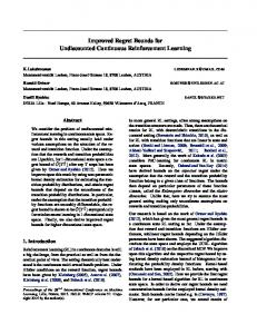
In this section we present some of the simulation results for several values of λ, C ( network capacity) and window Λ. The distribution π is taken to be U(0, 1). In this case, Garcia and Mari´c (2003) obtained that λ < 0.9282 is a sufficient condition for the simulation. The programs were written in MATLAB 5.0. For easiness of reading the results are presented in two steps: the clan of ancestors and the cleaning result. The basis of the rectangles kept at time t = 0 constitutes the perfect sample. 12

10

8

6

4

2

0

1

2

3

4

5

6

7

8

Figure 4.1: Clan of ancestors for U(0, 1), λ = 0.7, Λ = [0, 10].

11

9

12

10

8

6

4

2

0

1

2

3

4

5

6

7

8

9

1

2

3

4

5

6

7

8

9

12

10

8

6

4

2

0

Figure 4.2: Cleaning procedure for the clan presented in Figure 4.3. a) C = 1 b) C = 2.

12

5

Studying the characteristics of the clan of ances-

tors through simulation results We perform a 1,000 simulations for several values of λ < λ∗c . Conditioned on the event “the point (x, 0) is present at the free process” (which has probability 1 − exp{−λρ}), we observed

the values of N (A(x,0) ) – total number of rectangles present in the clan.

The expectations of this variable were estimated through the sample mean and compared then to the expected values for the associated branching process used to find the sub-criticality condition. The simulations were performed in two cases, when π is the U (0, 1) distribution and when π is concentrated in one point (fixed call length). From Garcia and Mari´c (2003), the critical value for λ to assure sub-criticality is • When π = U (0, 1)

• When π(d) = 1

λ∗c =

1 2

1 q + 13 λ∗c =

≈ 0.9282

1 2d

(5.1)

(5.2)

Graphic1: N (uniform) Figure 5 shows that the branching process dominates the clan of ancestors (we constructed then this way). However, due to the fact that in the branching process we can have subsequent generations of rectangles to be born in the same area as the predecessor generations, the number of rectangles of the branching process grows much faster than the number of rectangles of the clan of ancestors, as λ increases.

5.1

Estimation of the critical value using simulations

The purpose of this section is to study the behavior of the clan of ancestors as λ increases above λ∗c . From Figure 5 we can see that the critical value obtained through the domination by a branching process underestimates the true value of the finiteness of the clan of ancestors. The idea behind these results is to generate samples for increasing values of λ and to study the total

13

U(0,1)

15

Clan of ancestors Branching process

N

10

5

0

0.2

0.4

0.6

0.8

Lambda

d=0.5

80

60

N

Clan of ancestors Branching process

40

20

0

0.0

0.2

0.4

0.6 Lambda

0.8

1.0

Figure 5.3: Expected total number of rectangles in the branching process and the clan of ancestors. a) U(0, 1) b) d = 0.5

14

number of rectangles. Our conjecture is that, close to the true critical value λc the total number of rectangles should grow exponentially fast. Thus finding an assintote for E(N ) would give us an estimate of λc . This is true for the branching process, comparing the value of E(N ) as λ approaches λ∗c in Figure 5 we can see visually a vertical assintote at λ∗c . From now on, for all distributions, we sampled 1,000 observations of the clan of ancestors ¯ (the sample mean) for each value of λ. Figure 5.1 present the results for fixed and computed N length calls, d = 0.5.

1600

N

1200

800

400

0

0.0

0.5

1.0

1.5 Lambda

2.0

2.5

3.0

Figure 5.4: Expected number of rectangles in the clan of ancestors (E(N)) for d = 0.5 At first sight we see that there is an assintote close to 2.8. To be more precise, we tried to ¯ ) = 0 . We used a degree 19 polynomial to approximate find a root for the equation 1/ log(N ¯ ) and found a root in λ = 2.8231. 1/ log(N Several simulations were performed for several values of d just to get a more precise estimate for λc since due to the invariance of the Poisson process for fixed call length there is a linear relationship among the critical values for all d, see Table 5.1. Comparing the values of λ∗c =

1 2d

and λc we can see, as expected, a linear tendency and we

can adjust a regression model with no intercept using least squares to get

λc = 2.8246 ·

15

1 . 2d

(5.3)

d λc

0.5

1.0

1.4

2.0

2.5

3.0

3.5

4.0

4.5

5.0

2.8231 1.4193 1.0254 0.7312 0.5682 0.4537 0.3931 0.3530 0.3103 0.2833 Table 5.1: Critical value of λc obtained through simulation for several call lengths The question now is to perform the same comparison using different random distributions for

π. We simulated clan of ancestors for several Beta distributions and compared λ∗c and λc . Table 5.1 presents these results along with the ratio λc /λ∗c . We can see that λc ≈ 2.82λ∗c . Adjusting a least square model without any intercept: λc = 2.8243 λ∗c .

Distribution

λc

(5.4)

λc /λ∗c

U(0,1)

2.6135 2.8157

Beta(2,1)

2.0888 2.8695

Beta(2,2)

2.6746 2.8022

Beta(3,1)

1.8597 2.8353

Beta(3,2)

2.3079 2.8444

Beta(1,2)

3.7981 2.8166

Table 5.2: Critical value of λc obtained through simulation for distributions U(0, 1) and Beta(α, β)

6

Dominating the clan of ancestors by a 2-generation

branching process. Critical value. andez To construct the Galton-Watson process bn mentioned by the end of Section 3, Fern´ et al. (2001) used a multitype branching process Bn , in the set of cylinders, which dominates An . To do this they looked “backward in time” and let “ancestors” play the role of “branches”. In particular, births in the original marked Poisson process correspond to disappearance of branches. Like them, we reserve the words “birth” and “death” for the original forward-time

16

Poisson process. This construction can be done by enlarging the probability space and defining, i for any given set {R1 , . . . , Rk }, independent random sets BR 1 with the same marginal distribui tion as AR 1 . The important point here is that

k [

i=1

i AR 1 ⊂

k [

i BR 1 .

(6.1)

i=1

The procedure defined by B1 naturally induces a multitype branching process in the space of rectangles. The n-th generation of the branching process is defined by ′

R ′ R BR n = {B1 : R ∈ Bn−1 }

(6.2)

′

′

R where for all R′ , BR 1 has the same distribution as A1 and are independent random sets de-

pending only on R′ . Then, for all n ≥ 1 it follows R AR n ⊂ Bn .

(6.3)

It is introduced then a multitype branching process in the set of calls G. For an initial rectangle R with the basis of size u, bun is defined as the number of rectangles in the n-th generation of Bn that have basis with length v: ′

′

bun (v) = |{R ∈ BR n | |Basis (R )| = v}|.

(6.4)

The following relation is then established R |AR n | ≤ |Bn | =

X

bun (v).

(6.5)

v

We will have to further enlarge the set of types of Bn by creating a branching process in the set of cylinders B∗n with a new type called Color ∈ {b, g} which is inherited by a cylinder not only from the types of the first generation (parent) but also from the 2nd generation (grandparent). The types b, g are chosen to associate to black and green. The idea is to identify some rectangles in the branching process Bn that could never be present in the An . These rectangles we have in mind as “black”. Then, if the total number of “green” (not-black) rectangles is finite implies that the clan of ancestors is also finite. We expect then that counting only “green” rectangles one can obtain better critical value for λ. That is what

17

we are going to prove in the following.

For a rectangle V = (ξV , τV , sV , uV ) in the nth generation of the branching process Bn , we define an extra type to be its color as follows. For n = 1 or 2, Color (V ) = g. For n > 2, ′

R let R ∈ B∗n−1 and R′ ∈ B∗n−2 such that V ∈ BR 1 and R ∈ B1 . Denote R = (ξ, τ, s, u, c) and

R′ = (ξ ′ , τ ′ , s′ , u′ , c′ ), where c = Color (R) and c′ = Color (R′ ). Therefore, • if c = b then Color (V ) = b, • if c = g then Color (V ) = b

if and only if

D(uV , R, R′ ) = L(ξ, u, ξ ′ , u′ , uV ) × [0, τ ′ ] and

(ξV , τV + sV ) ∈ D(uV , R, R′ ) where

L(ξ, u, ξ ′ , u′ , uV ) = [max(ξ − uV , ξ ′ − uV ), min(ξ + u, ξ ′ + u′ )].

(6.6)

This way, for every rectangle is defined its bi-dimensional type Type (·) ∈ G × {b, g}. (w,c′ )

Consider dn

((u, c), (v, c′′ )) to be a 2-generation multitype branching process defined by

′

dn(w,c ) ((u, c), (v, c′′ ))

(6.7)

C = |{V : V ∈ BnC and R ∈ Bn−1 ; Type (C) = (w, c′ ), Type (R) = (u, c), Type (V ) = (v, c′′ )}|,

that is, it is the number of cylinders of type (v, c′′ ) in the nth generation of a cylinder of type (w, c′ ) which have an ancestor in the n − 1 generation of type (u, c). We can think of this branching process as a first order branching process with enlarged state space given by S = {((i, u, c), (j, v, c′′ ))} and offspring distribution to be Poisson distributed. From the definition of the process dn and the relation (6.5) it is clear that |AR n| ≤

X u,v

d(w,g) ((u, g), (v, g)) ≤ n

X

bw n (v).

(6.8)

v

We suppose from now on that π has discrete support. Proposition 6.9 In the process dn the mean number of offspring of type (u, c′′ ) of an individual of type (v, c) with the parent of type (w, c′ ) is given by    0, if c′ = b, c = b, c′′ = g or c′ = g, c = b, c′′ = g   m(((u′ , c′ ), (u, c)); ((u, c), (v, c′′ ))) = or c′ = b, c = g, c′′ = b or c′ = b, c = g, c′′ = g     λπ(v)(u + v), if c′ = b, c = b, c′′ = b or c′ = g, c = b, c′′ = b (6.10)

18

and 1 λπ(v)v, 2 v m(((u′ , g), (u, g)); ((u, g), (v, g)) ≤ λπ(v)(u + ) 2 m(((u′ , g), (u, g)); ((u, g), (v, b)) ≥

(6.11) (6.12)

Proof: For (6.10) it is enough to observe that from the definition of Color follows that is impossible to have green children from black parents. Since a black individual has all its children black, independently of its own parent type, the number of its children has the same low as the first generation in branching process bn defined by (6.4). The total number of children of a green individual has also the same low as the above one, but in this case it is possible to have children of both colors. Recall from (3.10) that E(bu (v)) = λπ(v)(u + v) so that m(((u′ , g), (u, g)); ((u, g), (v, b))) + m(((u′ , g), (u, g)); ((u, g), (v, g))) = λπ(v)(u + v).

(6.13)

Therefore, to prove (6.11) and (6.12) it is sufficient to find the mean number of black children from green parent (and necessarily green grandparent): m(((u′ , g), (u, g)); ((u, g), (v, b))). Consider two incompatible rectangles R = (ξ, τ, s, u, g) ∈ A2 and R′ = (ξ ′ , τ ′ , s′ , u′ , g) ∈ A1 ′

′ ′ such that R ∈ AR 1 , that is R is an ancestor of R . Since R belongs to the first generation, we

have τ ′ < 0 and τ ′ + s′ > 0. By construction of the clan of ancestors An and the branching

process Bn , rectangles R′ in the first generation have Birth (R′ ) < 0 and Death (R′ ) > 0. We want to compute the X(v, R, R′ )- number of black ancestors of v-type, namely the number ′

R of those V = (ξV , τV , sV , v) ∈ A3 with length v such that V ∈ AR 1 and R ∈ A1 . Let

Xb (v, R, R′ ) and Xa (v, R, R′ ) be the number of such ancestors that died before and after time t = 0, respectively. As before, let D ≡ D(v, R, R′ ) = L(ξ, u, ξ ′ , u′ , v) × [0, τ ′ ] and L ≡ L(ξ, u, ξ ′ , u′ , v) = [max(ξ − uV , ξ ′ − v), min(ξ + u, ξ ′ + u′ )].

(6.14)

X(v, R, R′ ) = Xb (v, R, R′ ) + Xa (v, R, R′ )

(6.15)

Then,

with P(Xb (v, R, R′ ) = k|u, τ, τ ′ ) = e−pb λ|D|

19

(−pb λ|D|)k k!

(6.16)

and P(Xa (v, R, R′ ) = k|u, τ, τ ′ ) = e−pa λ|L|

(−pa λ|L|)k k!

(6.17)

where pb is the probability that a rectangle who died in the area D is really an ancestral of R of type v, and analogously for pa . Therefore, pb = π(v)P(Y − S < τ )

(6.18)

′

= π(v)eτ (e−τ − 1)/(−τ ′ )

(6.19)

pa = π(v)P(−S < τ )

(6.20)

and

= π(v)eτ

(6.21)

where Y ∼ U (0, τ ′ ) (death time) and S ∼ exp(1) (lifetime) are independent random variables. We remind here that the rectangles are constructed in the negative time (“past”) so τ, τ ′ ≤ 0.

Given R and R′ , Xa (v, R, R′ ) and Xb (v, R, R′ ) are independent random variables, thus X(v, R, R′ ) is Poisson distributed with mean ′

π(v)(pb λ|D| + pa λ|L|) = π(v)λ|L|e(τ −τ ) .

(6.22)

Notice that τ < τ ′ and we are given the parent relation, so τ ′ −τ has exponential distribution

with mean one. Hence, E(e−(τ

′ −τ )

) = 1/2.

Furthermore, since ξ ∈ [ξ ′ − u, ξ ′ + u′ ] |L| = min(ξ + u, ξ ′ + u′ ) − max(ξ − v, ξ ′ − v) ≥ v

(6.23)

From (6.22) and the above inequality follows m(((u′ , g), (u, g)); ((u, g), (v, b))) = E(X(v, R, R′ )) ≥

1 λπ(v)v 2

(6.24)

And we have proved (6.11) as desired.

Sub-criticality: On account of the relation (6.8) we are interested in sub-criticality conditions for the green-type population of the branching process dn described above. Remember

20

that green individuals may appear in the n-th generation only as descendants of a branch made of green individuals only. Therefore, our aim is to establish conditions for the convergence of the series X X

m(n) (((w, g), (v, g)); ((vn−1 , g), (u, g)))

(6.25)

n≥1 vn−1 ,u

where m(1) (· ; ·) = m(· ; ·) is given by (6.11) and for n > 1 m(n) (((w, c′ ), (v, c)); ((v1 , c1 ), (u, c′′ ))) (6.26) X m(n−1) (((w, c′ ), (v, c)); ((v2 , c2 ), (v1 , c1 )))m(((v2 , c2 ), (v1 , c1 )); ((v1 , c1 ), (u, c′′ ))). = v2 ,c2

To simplify notation let m∗ (v, u) = λπ(u)(v + u2 )

(6.27)

and it follows from Proposition (6.9) that for all u, v and independently of w m(((w, g), (v, g)); ((v, g), (u, g))) ≤ m∗ (v, u).

(6.28)

Therefore, using the notation above and (3.10) we can easily estimate the series (6.25) to X

vn−1 ,u

m(n) (((w, g), (v, g)); ((vn−1 , g), (u, g))) ≤

= λn

P P

···

P

π(v1 )(v +

X

m(v, v1 )m∗ (v1 , v2 ) · · · m∗ (vn−1 , u) u,v1 ...vn−1

v1 )π(v2 ) v1 + v22 · · · π(u) vn−1 + u2 (6.29)

u

v1

X

 u ρ1 π(u) vn−1 + = vn−1 + = f1∗ + g1∗ vn−1 2 2

vn−1

Observe that

u

where f1∗ =

ρ1 2

(6.30)

and g1∗ = 1, and define inductively

X

vn−i+1

 vn−i+1  ∗ ∗ (fi−1 + gi−1 vn−i+1 ) = fi∗ + gi∗ vn−i . π(vn−i+1 ) vn−i + 2

Then we have j          ∗ fj∗ ρ1 /2 ρ2 /2 ρ1 /2 fj+1 ρ1 /2 ρ2 /2  ·  · =  = ∗ ∗ gj 1 ρ1 1 gj+1 1 ρ1

(6.31)

(6.32)

and consequently, the series (6.29) is equal to λn

X

∗ ∗ ∗ ∗ ∗ ∗ π(v1 )(v + v1 )(gn−1 v1 + fn−1 ) = λn (v(gn−1 ρ1 + fn−1 ) + ρ2 gn−1 + ρ1 fn−1 ).

v1

21

(6.33)



In order to find fn∗ , gn∗ we exponentiate T ∗ = 

ρ1 /2 ρ2 /2 1

ρ1

the eigenvalues of T ∗ , ε1 and ε2 given by

ε1,2 =

3ρ1 ±



. For this operation suffices

p

ρ21 + 8ρ2 . 4

and two corresponding normalized eigenvectors     ε1 − ρ1 ε2 − ρ1 1 1 , p .   p 1 + (ε1 − ρ1 )2 1 + (ε2 − ρ1 )2 1 1

(6.34)

(6.35)

From (6.32) it follows

fn∗ = gn∗ =

1 (εn (ε1 − ρ1 ) + εn2 (ρ1 − ε2 )) ε1 − ε2 1 1 (εn − εn2 ). ε1 − ε2 1

(6.36) (6.37)

Using the fact that |ε2 /ε1 | ≤ 1 in (6.33) and the Cauchy-Hadamard formula, we obtain that the radius of convergence of the series (6.29) is λ∗∗ c =

1 4 p = ε1 3ρ1 + ρ21 + 8ρ2

(6.38)

Therefore, as long as λ < λ∗∗ c the series (6.25) is absolutely convergent and consequently the green-type population of the process dn is almost surely finite. Calculation being done for countable number of types is not a real limitation. Namely, let V be the set of all possible types, by the same argument as used in Proposition 6.9 the mean number of green-type offspring in all generations is less then XZ

(n)

m∗ (v, du)

(6.39)

n≥1 V

where (n) m∗ (v, du)

=

Z

(n−1)

m∗ V

can be obtained inductively.

22

(v, dv ′ )m∗ (v ′ , du)

(6.40)

Suppose that the distribution of the length of the calls is absolutely continuous with respect to the Lebesgue measure and call π its density. We can write

m∗ (v, du) = λπ(du)(

du + v) 2

(6.41)

and the computation is completely analogous to the discrete case.

We summarize the results proved in this section in the following theorem: ∗∗ Theorem 6.42 If λ < λ∗∗ c , where λc is given by (6.38), then with probability one there is no

backward oriented percolation in R.

Remark: If π is the U (0, 1) density the condition becomes λ < 1.247 Observe the following relations: 4 2 4 ≥ λ∗∗ = λ∗c . √ c ≥ 3ρ1 3(ρ1 + ρ2 ) 3

(6.43)

The upper estimate in (6.43)is achieved in the case of just one type (fixed call length). The last inequality proves that a better bound for the critical value is obtained.

7

Conclusion

This is one of the first works where the clan of ancestors algorithm was implemented. Berthelsen and Møller (2002) compared it to the dominated CFTP introduced by Kendall and Møller (2000). Based on simulation results, they show that the dominated CFTP is better than the algorithm based on the clan of ancestors in the particular case of a Strauss process µΛ (dN ) =

1 β1 N (Λ)+β2 S(N,Λ) 0 e µΛ (dN ) ZΛ

(7.1)

defined on a unit square with eβ1 = 100 and eβ2 = 0 (the so-called hard-core process), 0.5 and 1 (a Poisson processes with rate 100). This is obviously the case from the description of the processes since the backward construction of BFA stops when the dominated Poisson process regenerates and usually the coupling of CFTP is achieved before it in the finite case.

23

However, it should be noticed that the algorithm based on the clan of ancestors was designed for sampling the infinite-volume process viewed in a finite window. This seems to be a much more interesting and challenging problem which has been studied in this work for the specific case of one-dimensional loss networks with bounded calls. No comparison was made to other perfect simulation schemes. Moreover, we can see that the simulation of the invariant measure can bring information about unknown variables related to the clan of ancestors. The bound described in Section 6 was found by a better understanding of the simulation procedure.

Acknowledgments We would like to thank Pablo Ferrari for many fruitful discussions. This work was partially funded by FAPESP Grant 00/01375-8 and CNPq Grant 301054/93-2.

References [1] Berthelsen, K.K. and Møller, J.(2002) A primer for perfect simulation for spatial point processes, Fifth Brazilian School in Probability (Ubatuba, 2001). Bull. Braz. Math. Soc. (N.S.) 33(3): 351–367. [2] Fern´ andez, R., Ferrari, P. A., Garcia, N. L. (2001). Loss network representation of Peierls contours, Annals of Probability 29(2): 902-937. [3] Fern´ andez, R., Ferrari, P. A., Garcia, N. L. (2002). Perfect simulation for interacting point processes, loss networks and Ising models. Stoch. Process. Appl. 102(1): 63-88. [4] Ferrari P. A., Garcia, N. L. (1998). One-dimensional loss networks and conditioned M/G/∞ queues. J. Appl. Probab. 35(4): 963-975. [5] Garcia, N. L., Mari´c, N. (2003). Ergodicity conditions for a continuous one-dimensional loss network. Bull. Braz. Math. Soc. 34(3): 349-360. [6] Hall, P. (1988). Introduction to the theory of coverage processes . John Wiley & Sons Inc., New York

24

[7] Kendall, W.S. and Møller, J. (2000) Perfect simulation using dominating processes on ordered spaces, with application to locally stable point processes. Adv. in Appl. Probab. 32(3): 844–865. [8] Kelly, F. P. (1991). Loss networks, Ann. Appl. Probab. 1(3): 319-378.

25