results are obtained with very affordable overheads in terms of space ... The domain-consistency obtained, called singleton- consistency ... We note D the domain of computation. ... names, points as tuples, and constraints as relations or tables.
Intelligence — Morgan Kaufmann, 2001
Improved bounds on the complexity of kB-consistency Lucas Bordeaux, Eric Monfroy, and Fr´ed´eric Benhamou IRIN, Universit´e de Nantes (France) {bordeaux, monfroy, benhamou}@irin.univ-nantes.fr
Abstract kB-consistencies form the class of strong consistencies used in interval constraint programming. We survey, prove, and give theoretical motivations to some technical improvements to a naive kBconsistency algorithm. Our contribution is twofold: on the one hand, we introduce an optimal 3Bconsistency algorithm whose time-complexity of O(md2 n) improves the known bound by a factor n (m is the number of constraints, n is the number of variables, and d is the maximal size of the intervals of the box). On the other hand, we prove that improved bounds on time complexity can effectively be reached for higher values of k. These results are obtained with very affordable overheads in terms of space complexity. Keywords: Strong consistency techniques, Interval constraint propagation.
1 Introduction Consistency algorithms are polynomial techniques which aim at struggling against the combinatorial explosion of bruteforce search by reducing the search space. Among them, strong consistencies [Freuder, 1978] denote generic algorithms which can be tuned to enforce arbitrary intermediate levels of consistency. One of the most (if not the most) promising strong consistency techniques is the class of kBconsistencies, where k may vary from 2 to a maximum value corresponding to global consistency. kB-consistency was introduced in [Lhomme, 1993] as a response to the problem called early quiescence [Davis, 1987]: when applied to non-trivial, real-valued problems, filtering techniques adapted from arc-consistency do not reduce the search space enough in practice, and stronger consistencies are thus needed to limit the size of the search tree. The basic idea is that given a solver of level k − 1, each possible value of the variables can be enumerated; if the k − 1 solver proves the inconsistency of the problem obtained when variable x is instantiated to value v, we know that v is not a possible value for x. This method can be applied to both domainbased solvers (by suppressing inconsistent values from domains) and interval-based solvers (by tightening bounds).
The domain-consistency obtained, called singletonconsistency has been emphasized as one of the most efficient techniques for hard finite-domain problems [Debruyne and Bessi`ere, 1997]. This paper deals with the interval-consistency obtained, called kB-consistency. kB-consistency has been successfully applied to difficult nonlinear problems, such as a challenging transistor design application [Puget and van Hentenryck, 1998]. The important advantage of kB over path-consistency [Montanari, 1974] and its variants [Dechter and van Beek, 1996; Sam-Haroud and Faltings, 1996] is that it does not require the use of the costly multi-dimensional representations of the constraints needed in these methods. Let d be the number of elements in the widest initial interval, n be the number of variables, and m be the number of constraints; the known bound of time-complexity for computing kB-consistency is O(mdk−1 n2(k−2) ): 2B is computed in O(md) and each increase in the factor k has a cost of O(dn2 ). Our aim is to show that this complexity is overestimated and that the expected optimum is actually O(mdk−1 nk−2 ). We show that this bound can be approached in the general case and that it can be exactly reached in the especially interesting case of 3B. This result is obtained by a cautious formulation of the algorithm, in which an optimization pointed out by Lhomme and Lebbah [Lebbah, 1999] is integrated. Informally speaking, each time an interval is reduced, the k − 1 solver performs an incomplete computation. The optimization is to store the result of this computation, so that successive calls to the solver do not need to be restarted from scratch. A dynamic dependency condition is used to determine that some operations can be avoided. We then study the cost of the cumulation of all these incomplete computations to find improved bounds on time complexity. The outline of this paper is the following: next section introduces the required material and terminology on constraints and solvers. Section 3 introduces interval consistency techniques and in particular kB-consistency. We then define and prove two improvements to a naive algorithm for computing it (Section 4). A theoretical analysis of the resulting algorithm allows us to state the new complexity results in Section 5, while the end of the paper is concerned with conclusions and perspectives.
2 Constraints and Solvers We note D the domain of computation. D is supposed to be finite and totally ordered: it is thus possible to compute the predecessor and the successor of any element v. This assumption may seem very restrictive, but it corresponds to the usual representation of numbers with computers: in practice, D is either the set of the canonical floating-point intervals or the subset of the integers encoded on a given number of bits.
2.1
Basic terminology
Let V be a finite set of variables. A point t is defined by a coordinate tx on each variable x, i.e., points are mappings from V to D. A constraint c is a set of tuples. For readers more familiar with database-theoretic concepts [Dechter and van Beek, 1996], variables may also be thought of as field names, points as tuples, and constraints as relations or tables. Points may also be seen as logical valuations. A CSP C is a set of constraints. The set of solutions to C is the set Sol(C) ofTthe points which belong to all its constraints, i.e., Sol(C) = {c | c ∈ C}. The problem of constraint satisfaction is to find (one/all) solution(s) to a CSP. It is a NPcomplete problem in its decisional form. The cut σx=v (c) of a set of points c is the set containing the points of c whose coordinate on x is v: σx=v (c) = {t ∈ c | tx = v}. It is also referred to as the selection or instantiation operator. Among other properties, this operator is monotonic: c ⊆ c′ ⇒ σx=v (c) ⊆ σx=v (c′ ). Though these definitions are fully general and do not depend on the way constraints are expressed, some points in this paper are concerned with the special case of systems of equations and inequations over D. As an example of such systems, {1/x + 1/y = z, x = y} defines the CSP C = {c1 , c2 } where c1 = {hx, y, zi | 1/x + 1/y = z} and c2 = {hx, y, zi | x = y}. A solution is hx = 2, y = 2, z = 1i. The cut σz=1 (c1 ) defines the set {hx, y, 1i | 1/x + 1/y = 1}. Notations: Throughout the text, the considered CSP will be fixed and called C; consequently we shall omit this parameter in most definitions.
2.2
Interval-consistency
We call search space (Ω) the set of points among which solutions are searched for. In the interval-consistency framework [Benhamou and Older, 1997], the search space is the cartesian product of intervals associated to every variable. The success of this representation comes from the fact that it is a compact and expressive way to approximate the solutions. We note lbx and ubx the lower and upper bounds of the interval of possible values for variable x. The search space is thus the set containing the points t whose coordinates are inside the bounds (∀x ∈ V, tx ∈ [lbx , ubx ]). It is called a box, due to the obvious geometric intuition. When we refer to a bound bx without further detail, it can be indifferently the lower or the upper bound of x. An intuitive way to reason on bounds is by relating them to the facets of the box. Formally, a facet is the set of points of the box whose coordinate on a given variable is fixed to a bound: it can be written σx=bx (Ω) for some variable x and some bound bx of x.
Notations: Given a box Ω, we note consistent(Ω) the property Ω ∩ Sol(C) = 6 ∅, which states that Ω contains a solution.
2.3
Solvers
We define (constraint) solvers as functions which verify the following properties: Definition 1. [Solver] A solver is a function Φ on boxes such that: Φ(Ω) ⊆ Ω (contractance) Φ(Ω) ⊇ Ω ∩ Sol(C) (correctness) Ω ⊆ Ω′ ⇒ Φ(Ω) ⊆ Φ(Ω′ ) (monotonicity) Φ(Φ(Ω)) = Φ(Ω) (idempotence) Note that we deliberately exclude the case of nonidempotent solvers, which are not relevant here. Solvers are intended to reduce the search space; the key-point is that they are usually integrated within a branch and prune algorithm, which is guaranteed to find the solutions only if the solver does not remove any of them, hence we call this essential property correctness. The opposite property to correctness is completeness, which states the implication ¬consistent(Ω) ⇒ Φ(Ω) = ∅. Complete solvers are able to detect all inconsistencies, but are usually too costly to be considered practically.
3 kB-consistency The solvers we now consider can be seen as functions which tighten the intervals by modifying each bound in turn; we often refer to this process as facet reduction, meaning that facets are “pushed down”. Solvers are defined via local consistency properties, which characterize the facets obtained when the reduction stops. We now define kB-consistency inductively, starting with a basic consistency technique for the case k = 2.
3.1
2B-consistency
2B-consistency is also called hull-consistency by some authors [Benhamou and Older, 1997]. On finite domains, it is the core of some of the main constraint logic programming solvers [Van Hentenryck et al., 1998; Codognet and Diaz, 1996], and it is often referred to as partial lookahead. Definition 2. [2B-consistency] A box Ω is 2B-consistent if for every bound bx we have: ∀c ∈ C, σx=bx (Ω) ∩ c 6= ∅ The 2B-consistency solver is the function Φ2 which maps a box Ω to the greatest 2B-consistent box included in Ω. This definition means that bounds are reduced until each facet of the box intersects every constraint. It can be proved that Φ2 is a valid function: the computed greatest box exists and is unique; this result comes from more general properties of confluence of fixpoint computations [Apt, 1999]. Furthermore, Φ2 is a valid solver: correctness holds because a value v is suppressed from a variable x if ∃c ∈ C, σx=v (C)∩c = ∅, so that we have ¬consistent(σx=v (C)), which proves that the solver only removes facets which do not contain solutions; idempotence is straightforward and monotonicity comes from the monotonicity of the selection operator.
2B-consistency can only be computed for some special constraints called primitive, which correspond to the basic arithmetic relations defined by the language. Solvers like Prolog IV decompose arbitrary constraints (e.g., (2 + x).y = z) into such primitive constraints (2+x = x′ , x′ y = y ′ , y ′ = x).
3.2
kB-consistency
The condition that every facet intersects every constraint is a very rough approximation of (global) consistency. kBconsistency relies on the observation that ideally, a facet should be reduced until it contains a solution; since deciding whether a facet contains a solution is itself a constraint satisfaction problem, a solver Φk−1 can do for this task. Definition 3. [kB-consistency] A box Ω is kB-consistent (for k ≥ 3) if for every bound bx we have: Φk−1 (σx=bx (Ω)) 6= ∅ The kB consistency solver is the function Φk such that the box Φk (Ω) is the greatest kB-consistent box included in Ω. Informally speaking, bounds are reduced until no facet is rejected by the solver Φk−1 . This definition is recursive: 3Bconsistency uses the 2B-consistency solver and can in turn be used to define 4B-consistency, and so on. Properties of confluence, idempotence and monotonicity hold for Φk . Its correctness is a consequence of the correctness of Φk−1 : since Φk−1 (σx=bx (Ω)) = ∅ implies ¬consistent(C), the removed facets do not contain any solution. It is easy to prove that Φk is “stronger” than Φk−1 , i.e., that Φk (Ω) ⊆ Φk−1 (Ω) (this is due to the monotonicity of Φk−1 ). Note that the idea of kB-consistency can be customized and that any consistency technique can be used instead of 2Bconsistency. Some authors have considered the use of Boxconsistency [Puget and van Hentenryck, 1998] or lazy forms of arc-consistency [Debruyne and Bessi`ere, 1997].
1 Q := C 2 while Q 6= do 3 Q := Q − {c} % arbitrary choice of c 4 for each variable x constrained by c do 5 reduce lbx while σx=lbx (Ω) ∩ c = 6 reduce ubx while σx=ubx (Ω) ∩ c = 7 if [lbx , ubx ] has been modified then 8 Q := Q ∪ {c′ ∈ C | c′ depends on x, c′ 6= c}
?
? ?
Figure 1: The algorithm for 2B-consistency • In the case of numeric constraints, each constraint depends on (at most) 3 variables; • Lines 5 and 6 of the algorithm can be performed in bounded time using interval computations.
4.2
Naive algorithm for kB-consistency
The filtering of a box Ω by kB-consistency is computed by reducing each of its facets in turn. In the following algorithm (Figure 2) we use the notation reduce . . . while to represent the computation of the new bound. This notation actually represents a loop: while the specified condition does not hold, the bound is iteratively reduced to the next (when reducing a lower bound) or previous (upper bound) element. This loop may indeed be optimized, for instance by trying to remove several values at once, or even by using recursive splitting. Unfortunately, these heuristics do not improve the worst-case complexity: at worst, every value has to be considered in turn to be effectively reduced. 1 do 2 for each bound bx do 3 reduce bx while Φk−1 (σx=bx (Ω)) = 4 while Ω is changed
?
Figure 2: Naive algorithm for kB-consistency
4 Algorithms We now present the algorithms for computing kBconsistency. As far as 2B-consistency is concerned, we only sketch the notions required to understand the subsequent proofs, and the reader is referred to [Benhamou and Older, 1997; Lhomme, 1993] for further explanations. We then give an incremental description of the algorithm for kB-consistency in the general case: starting from a naive algorithm, we successively describe two optimizations used by the experts of this technique and suggested in [Lebbah, 1999] (see also [Delobel, 2000]). The theoretical interest of these improvements shall be studied in the next section.
4.1
The correctness of this algorithm is straightforward since when the while loop stops, all the bounds are kB-consistent.
4.3
Storing information
The most obvious drawback of the preceding algorithm is that each time a facet σx=bx (Ω) is reconsidered, the solver Φk−1 is restarted from scratch to reduce it. A more clever approach is to store the result of this reduction, in order to reuse it in the next steps (Figure 3). The notation memorize is a simple assignment, but it is intended to express the fact that the memorized box has already been computed in the previous line.
Computing 2B-consistency
The algorithm for enforcing 2B-consistency is a variant of the seminal propagation algorithm - AC3. It is a “constraintoriented” algorithm, which handles a set of constraints to be considered (generally stored as a queue). It relies on the fact that every constraint c relates a given number of variables we say that c depends on this variable x, or alternatively that c constrains x. Figure 1 describes the algorithm. Two points are essential to the complexity study:
1 for each bound bx do mem[bx ] := Ω 2 do 3 for each bound bx do 4 mem[bx ] := Φk−1 (mem[bx ] ∩ Ω) 5 if mem[bx ] = then 6 reduce bx while Φk−1 (σx=bx (Ω)) = 7 memorize Φk−1 (σx=bx (Ω)) into mem[bx ] 8 while Ω is changed
?
Figure 3: kB algorithm with storage
?
We use a vector mem1 which associates to every bound the last non-empty box computed while reducing it. When a bound bx is reconsidered, it is possible to restart the solver from the box mem[bx ] ∩ Ω (cf. Line 4), because we have: Φk−1 (σx=bx (Ω)) = Φk−1 (mem[bx ] ∩ Ω) Proof. Note that the intersection mem[bx ] ∩ Ω is a way to rewrite mem[bx ] ∩ σx=bx (Ω) since mem[bx ] contains only points with value bx on x. Since mem[bx ] = Φk−1 (σx=bx (Ω′ )) for some Ω′ ⊇ Ω, a direct consequence of monotonicity is that Φk−1 (σx=bx (Ω)) ⊆ mem[bx ]. We also have Φk−1 (σx=bx (Ω)) ⊆ σx=bx (Ω) (contractance), and thus Φk−1 (σx=bx (Ω)) ⊆ mem[bx ] ∩ σx=bx (Ω)). Using monotonicity and idempotence we prove that Φk−1 (σx=bx (Ω)) ⊆ Φk−1 (mem[bx ] ∩ σx=bx (Ω)) = Φk−1 (mem[bx ] ∩ Ω). The other inclusion ⊇ is straightforward.
4.4
Avoiding computation
The second optimization relies on the observation that it is not worth recomputing a bound bx if mem[bx ] ⊆ Ω, because mem[bx ] ∩ Ω is then equal to mem[bx ] which is already a fixpoint of the solver Φk−1 . In the algorithm of Figure 4, this condition is checked in a naive fashion before each bound reduction: 1 for each bound bx do mem[bx ] := Ω 2 do 3 for each bound bx do 4 if mem[bx ] 6⊆ Ω then 5 mem[bx ] := Φk−1 (mem[bx ] ∩ Ω) 6 if mem[bx ] = then 7 reduce bx while Φk−1 (σx=bx (Ω)) = 8 memorize Φk−1 (σx=bx (Ω)) into mem[bx ] 9 while Ω is changed
?
?
Figure 4: Algorithm with dynamic dependency checkings Figure 5 is an illustration of the preceding considerations: in this figure, bound ubx is reduced but the global box still contains mem[lby ] (= Φk−1 (σy=lby (Ω′ )) for some box Ω′ ⊇ Ω). The re-computation of bound lbx can therefore be avoided.
5 Complexity analysis This section is concerned with the theoretical study of the algorithms, starting with the special case of 2B-consistency. We then study the complexity of the algorithms of Section 4, and point out little improvements needed to compute kB in near-optimal time. As a comparison, we first recall the original complexity results given in [Lhomme, 1993]. As usual in the literature [Mackworth and Freuder, 1985 ], the complexity of local consistency algorithms is expressed as a function of the following parameters: 1
Technically, bounds may be seen as variables, it is thus legitimate to use their value (c.f. σx=bx (Ω)) or to modify them (as in “reduce bx while”). Our use of the notation mem[bx ] is slightly abusive, the intended meaning is that the stored value is associated to the bound, not to its current value.
reduction
the facet σy=lby (Ω)
mem[lby ] = Φk−1(σy=lby (Ω ′)) lbx
uby ubx
lby
Figure 5: An illustration of the algorithms • n = |V| the number of variables, • m = |C| the number of constraints, • d the number of elements in the greatest interval of the box. In general, it is possible to artificially define as many constraints as is wished on a given number of variables. On the contrary, it is not possible to have n > 3m (for ternary constraints) unless the absurd case of disconnected constraint graphs is accepted, thus n = O(m).
5.1
Complexity of 2B-consistency
The complexity of 2B-consistency has been determined by [Lhomme, 1993] using an argument inspired from [Mackworth and Freuder, 1985 ]. We recall this result and give a simpler proof: Complexity 1. The time-complexity for the algorithm computing 2B-consistency (see Figure 1) is O(md). Proof. Between two insertions of a constraint c into the set Q, the reduction of one of the intervals on which c depends must have occurred. c depends on a bounded number of variables (3 in our case), and each interval may be reduced at most d times. The overall number of insertions of a given constraint into the queue is hence bounded by O(d), and the number of insertions of the m constraints is O(md). Since Lines 5 and 6 of the algorithm require constant time, this gives the complexity. We also recall the best-case running time: when no reduction is obtained (the box is already 2B-Consistent), every constraint is dequeued in time Θ(m).
5.2
Complexity of the original algorithm
The complexity of the original algorithm for kB-consistency presented in [Lhomme, 1993] is the same as the one of the naive algorithm presented in Figure 2. To show that this algorithm runs in time O(mdk−1 n2(k−2) ), we just prove the following result: Complexity 2. The number of calls to the solver Φk−1 in the naive kB-consistency algorithm is O(dn2 ).
Proof. The worst case is obtained when re-computing all facets (Line 2 of the algorithm of Figure 2) results in a minimal reduction (removal of one element) of only one of the bounds: consequently, O(n) applications of Φk−1 are needed to remove one element. Since one interval is associated to each of the n variables, dn elements may be suppressed one after the other in the worst case, hence the overall number of applications of the solver Φk−1 is O(dn2 ). Note that this complexity does not seem to be optimal: since we use the solver Φk−1 to test each element of every variable, we could expect an optimal algorithm to perform only O(dn) calls to Φk−1 . We shall see how this presumably optimal bound can be reached in the case of 3B-consistency.
5.3
3B-consistency
We now have all the theoretical elements at hand for a critical study of the algorithm of Figure 4. We first restrict ourselves to the case of 3B-consistency, whose expected optimal complexity is O(md2 n). The algorithm of Figure 4 is not optimal yet for a simple reason: to suppress some value on a given interval, it may be needed to apply several 2B-consistencies, each time with cost O(m). The problem is that 2B is run on all constraints in a systematic way, while only the ones which depend on a bound which has been reduced since the last run should be enqueued. This situation may be avoided with a finer storage of the queues used by 2B-consistency (Figure 6): a queue q[bx ] is attached to each facet bx , and each time the reduction of a facet stops, the corresponding queue is empty. Only the constraints which effectively have to be reconsidered are enqueued (Line 12). In the following the expression using means that Φ2 is run with q[bx ] as an initial queue instead of the queue containing all the constraints used in Figure 1:
Proof. Several calls to the solver Φ2 may be required to suppress a value v from a given variable. Throughout these calls, each constraint is taken into account only if one of the variables on which it depends has been reduced (either during the current computation of 2B-consistency or between the previous computation and the current one). The cumulated number of constraint insertions into the queue for all the calls related to value v is then bounded by O(md). Since O(dn) such values may be suppressed, the global cost is O(md2 n). This bound is correct because the number of tests of interval inclusions has been optimized: in the algorithm, O(n) interval inclusions are checked every time one of the O(dn) elements is effectively removed, and the cost of these tests is then O(dn2 ). Since n is O(m), this complexity is less than O(md2 n).
5.4
Complexity of kB-consistency
We refine the analysis of the complexity of kB-consistency. Figure 7 shows the savings obtained by the memorization presented before. Ω1 is a facet of some box. It is reduced by (k − 1)B-consistency in order to show that the corresponding value v is inconsistent. The values suppressed by (k − 2)Bconsistency appear as tiles on the figure. The second part of the figure shows a case where the search space Ω′ has been reduced and the re-computation of (k − 1)B-consistency is needed.
mem[bx ] = Φk−1 (Ω1 ) 1
1 2 3 4 5 6 7 8 9 10 11 12 13
for each bound bx do mem[bx ] := Ω q[bx ] := C do for each bound bx do mem[bx ] := Φ2 (mem[bx ]) using q[bx ] if mem[bx ] = then reduce bx while Φ2 (σx=bx (Ω)) = memorize Φ2 (σx=bx (Ω)) into mem[bx ] for each bound by do if mem[by ] 6⊆ Ω then mem[by ] := mem[by ] ∩ Ω q[by ] := q[by ] ∪ {c | c depends on bx } while Ω is changed
?
?
Figure 6: Optimized handling of the queues in 3B Note that this algorithm is essentially the same as the one of Figure 4 where the test for inclusion in Line 10 and the intersection in Line 11 are applied in an optimized way. These two operations can be especially easily computed since only the interval for the variable x which has effectively been changed has to be checked or reduced. Complexity 3. The algorithm of Figure 6 is optimal (O(md2 n)).
mem[bx ] = Φk−1 (Ω2 )
σx=bx (Ω ′ )
Ω1 = σx=bx (Ω)
2
Ω2
3
Ω2
Figure 7: Successive reductions of a facet σx=v (Ω). To determine the complexity of kB-consistency, we bound the number of filterings by (k − 2)B-consistency (i.e. the tiles). The keypoint is that the algorithm stores the suppressions obtained by (k − 2)B, and avoids computing them several times. We have the following result: Complexity 4. When computing kB-consistency, the number of computations of (k − 2)B-consistency is O(d2 n3 ). Proof. Consider the computation needed to suppress some value v associated to a variable x (v may be thought of as the bound bx of the box). O(dn) such values exist. Due to the memorization, it is needed to re-compute the (k − 1)Bconsistency on the facet σx=v (Ω) only in the case where one of the values of the corresponding memorized box (mem[bx]) has been removed. In the worst case, it may happen that no computation of (k − 1)B-consistency reduces the memory; up to O(dn) such computations can thus occur, since O(dn) suppressions of a single value of the memory may occur. Each time, the number of (k − 2)B-consistencies that are checked is O(n) (one is run on each facet of σx=v (Ω)).
The overall number of (k − 2)B-consistencies is bounded by O(d2 n3 ). Since the original bound on the number of (k − 2)Bconsistencies is O(d2 n4 ), we have shown an improvement of the worst-case behaviour. We summarize the results for 2B, 3B, and stronger consistencies (k ′ ≥ 1): (2k ′ )B (2k ′ + 1)B
′
O(md.(d2 n3 )k −1 ) ′ O(md2 n.(d2 n3 )k −1 )
6 Conclusion Investigating several improvements to a basic algorithm for computing kB-consistency, we have designed an optimal algorithm for 3B-consistency, and shown that improved bounds are reached for higher values of k. Note that the algorithms presented here are very affordable in terms of space complexity: the storage of the boxes needed by the algorithms of Figures 4 and 6 requires space O(kn2 ) (n2 space is needed to store a box for each facet at each level and no two applications of some solver for the same level of k may coexist). The handling of the queues in the algorithm of Figure 6 requires O(nm) additional space. In terms of algorithms, our main contribution was to overview and justify theoretically some improvements based on some memorization of computation. Though our purpose was not to discuss the practical relevance of this technique, it actually proves to be effective on our implementation, since it allows saving some percents of the computations of facets. Typical benchmarks show that 5% to 60% of the facet reduction may be avoided while computing 3B-consistency. It might be possible to generalize these memorization techniques to each level of kB-consistency, and hence to improve the theoretical time-complexity - to the detriment of spacecomplexity. Our study of the complexity of interval consistency techniques may be regarded as complementary to the qualitative results which compare the filtering obtained by the algorithms. For instance, it is well-known that 3B-consistency allows to compute more precise intervals than Box-consistency [Collavizza et al., 1999], but that it is also a more costly technique. Since the efficiency of constraint solving depends on the compromise between the pruning obtained and the time required to achieve it, an interesting perspective is to study the difference between the two algorithms in terms of theoretical costs. Note that our study was restricted to the original definition of kB-consistency, and that the alternative definition based on Box-consistency introduced in [Puget and van Hentenryck, 1998] has not been considered. Since Box-consistency is computed in a very similar way to 2B, it seems however that little customization of our algorithm is needed to handle this case. A more challenging task would be to determine whether similar optimizations to the ones presented in this paper may be helpful in the combinatorial case, where domains are considered instead of intervals. Acknowledgements We express our gratitude to Olivier Lhomme for its encouragements and advice.
References [Apt, 1999] K. Apt. The essence of constraint propagation. Theoretical Computer Science, 221(1-2), 1999. [Benhamou and Older, 1997] F. Benhamou and W. Older. Applying interval arithmetic to real, integer and boolean constraints. Journal of Logic Programming, 32(1), 1997. [Codognet and Diaz, 1996] P. Codognet and D. Diaz. Compiling constraints in clp(fd). Journal of Logic Programming, 27(3), 1996. [Collavizza et al., 1999] H. Collavizza, F. Delobel, and M. Rueher. Comparing partial consistencies. Reliable Computing, 5(3), 1999. [Davis, 1987] E. Davis. Constraint propagation with interval labels. Artificial Intelligence, 32, 1987. [Debruyne and Bessi`ere, 1997] R. Debruyne and C. Bessi`ere. Some practicable filtering techniques for the constraint satisfaction problem. In Proceedings of the 15th IJCAI, Nagoya, Japan, 1997. [Dechter and van Beek, 1996] R. Dechter and P. van Beek. Local and global relational consistency. Theoretical Computer Science, 173(1), 1996. [Delobel, 2000] F. Delobel. R´esolution de contraintes r´eelles non-lin´eaires. PhD thesis, Universit´e de Nice - Sophia Antipolis, 2000. [Freuder, 1978] E.C. Freuder. Synthesising constraint expressions. Communications of the ACM, 21, 1978. [Lebbah, 1999] Y. Lebbah. Contribution a` la r´esolution de contraintes par consistance forte (in french). PhD thesis, ENSTI des Mines de Nantes, 1999. [Lhomme, 1993] O. Lhomme. Consistency techniques for numeric CSPs. In Proceedings of the 13th IJCAI, pages 232–238, Chamb´ery, France, 1993. [Mackworth and Freuder, 1985 ] A. Mackworth and E. Freuder. The complexity of some polynomial network consistency algorithms for constraint satisfaction problems. Artificial Intelligence, 25(1), 1985. [Montanari, 1974] U. Montanari. Networks of constraints: Fundamental properties and applications to picture processing. Information Science, 7(2), 1974. [Puget and van Hentenryck, 1998] J.-F. Puget and P. van Hentenryck. A constraint satisfaction approach to a circuit design problem. Journal of Global Optimization, 13, 1998. [Sam-Haroud and Faltings, 1996] J. Sam-Haroud and B. V. Faltings. Consistency techniques for continuous constraints. Constraints, 1, 1996. [Van Hentenryck et al., 1998] P. Van Hentenryck, V. Saraswat, and Y. Deville. Design, implementation and evaluation of the constraint language cc(fd). Journal of Logic Programming, 37(1-3), 1998.