Improved Inference for Moving Average Disturbances in Nonlinear ...

Hindawi Publishing Corporation Journal of Probability and Statistics Volume 2014, Article ID 207087, 12 pages http://dx.doi.org/10.1155/2014/207087

Research Article Improved Inference for Moving Average Disturbances in Nonlinear Regression Models Pierre Nguimkeu Department of Economics, Andrew Young School of Policy Studies, Georgia State University, P.O. Box 3992, Atlanta, GA 30302-3992, USA Correspondence should be addressed to Pierre Nguimkeu; [email protected] Received 30 August 2013; Revised 22 November 2013; Accepted 14 December 2013; Published 13 February 2014 Academic Editor: Shein-chung Chow Copyright © 2014 Pierre Nguimkeu. This is an open access article distributed under the Creative Commons Attribution License, which permits unrestricted use, distribution, and reproduction in any medium, provided the original work is properly cited. This paper proposes an improved likelihood-based method to test for first-order moving average in the disturbances of nonlinear regression models. The proposed method has a third-order distributional accuracy which makes it particularly attractive for inference in small sample sizes models. Compared to the commonly used first-order methods such as likelihood ratio and Wald tests which rely on large samples and asymptotic properties of the maximum likelihood estimation, the proposed method has remarkable accuracy. Monte Carlo simulations are provided to show how the proposed method outperforms the existing ones. Two empirical examples including a power regression model of aggregate consumption and a Gompertz growth model of mobile cellular usage in the US are presented to illustrate the implementation and usefulness of the proposed method in practice.

1. Introduction Consider the general nonlinear regression model defined by 𝑦𝑡 = 𝑔 (𝑥𝑡 ; 𝛽) + 𝑢𝑡 ,

(1)

where 𝑥𝑡 = (𝑥𝑡1 , . . . , 𝑥𝑡𝑘 )󸀠 is a 𝑘-dimensional vector of regressors and 𝛽 = (𝛽1 , . . . , 𝛽𝑘 )󸀠 is a 𝑘-dimensional vector of unknown parameters. The regression function 𝑔(⋅) is a known real-valued measurable function. Nguimkeu and Rekkas [1] proposed a third-order procedure to accurately test for autocorrelation in the disturbances, 𝑢𝑡 , of the nonlinear regression model (1) when only few data are available. In this paper we show how the same approach can be used to test for first-order moving average, MA(1), disturbances in such models. We therefore assume in the present framework that the disturbance term 𝑢𝑡 in Model (1) follows a first-order moving average process, MA(1), 𝑢𝑡 = 𝜖𝑡 + 𝛾𝜖𝑡−1 ,

(2)

where the error terms 𝜖𝑡 are independently and normally distributed with mean 0 and variance 𝜎2 and the process 𝑢𝑡 is stationary and invertible with |𝛾| < 1.

Although regression models with moving average disturbances are surely no less plausible a priori than autoregressive ones, they have been less commonly employed in applied research. The main reason for this lack of interest has been argued by some authors, for example, Nicholls et al. [2], as the computational difficulty in estimating these models. However, with the recent improvements in computer capabilities and numerical algorithms, such concerns have been greatly alleviated. Unlike in an autocorrelated error process where all error terms are correlated, the MA(1) error process allows correlation between only the current period and the next period error terms. This feature of the MA(1) error process makes it very attractive in situations where precisely this type of correlation structure is more appropriate and instructive. Many real data applications can be found in Franses [3], Hamilton [4], and L¨utkepohl and Kratzig [5]. The method proposed in this paper is based on a general theory recently developed by Fraser and Reid [6] and possesses high distributional accuracy as the rate of convergence is 𝑂(𝑛−3/2 ) whereas the available traditional asymptotic methods converge at rate 𝑂(𝑛−1/2 ). The proposed method is accordingly referred to as third-order method and its

2

Journal of Probability and Statistics

feature makes it more convenient and particularly attractive for small sample size models. The approach proposed in this paper is also a general procedure for which the Chang et al. [7] statistics, designed for testing moving average in pure univariate time series, is a special case. More specifically, Chang et al. [7] assumed the mean to be some constant 𝜇 whereas the current paper considers a general form for the mean function to be 𝑔(𝑥𝑡 , 𝛽), where 𝛽 is a vector of unknown parameters and the function 𝑔(⋅, ⋅) is known. Although the parameter of interest 𝛾 exists only in the variance-covariance matrix of the error terms and may seem unrelated to the mean function at first, estimation of 𝛾 in regression analysis provides estimates that depend on both the estimates and the functional form of the mean function. Hence, inference about 𝛾 crucially relies on the nature of 𝑔(𝑥𝑡 , 𝛽). This paper proposes a general procedure that accommodates various forms of the regression functions 𝑔(𝑥𝑡 , 𝛽) including nonlinear, linear, or constant functions. In Section 2, we discuss the nonlinear regression model with MA(1) errors and explain how the 𝑝-value function for the correlation parameter of interest, 𝛾, can be obtained. We also show how the proposed method can be adopted for a more general higher-order moving average process. For a thorough exposition of the background methodology of third-order inference, we refer the reader to the discussions in Fraser and Reid [6] and Fraser et al. [8]. Numerical studies including Monte Carlo simulations as well as real data applications on aggregate consumption and mobile cellular usage in the US are presented in Section 3 to illustrate the superior accuracy of the proposed method over existing ones and its usefulness in practice. Finally, some concluding remarks are given in Section 4.

2. The Model and the Proposed Method

𝛾 1 + 𝛾2 𝛾 1 + 𝛾2 𝑊 = 𝑊 (𝛾) = ( 0 .. .

𝛾 .. .

( 0

0

2.1. Model and Estimation. Using NR notation we can rewrite the nonlinear regression model (1) with error terms defined by (2) in a reduced matrix form. Denote by𝑦 = (𝑦1 , . . . , 𝑦𝑛 )󸀠 the vector of observations of the dependent variable 𝑦𝑡 , 𝑔(𝑥, 𝛽) = (𝑔(𝑥1 , 𝛽), . . . , 𝑔(𝑥𝑛 , 𝛽))󸀠 the regression vector evaluated at 𝑥 = (𝑥1 , . . . , 𝑥𝑛 )󸀠 , and 𝑢 = (𝑢1 , . . . , 𝑢𝑛 )󸀠 the vector of error terms. Then Model (1) with error terms defined by (2) can be rewritten as (3)

with

0 𝛾

1 + 𝛾2 d d ⋅⋅⋅

(4)

0 0 .. . ).

d 𝛾 𝛾 1 + 𝛾2 )

󸀠

Denote by 𝜃 = (𝛾, 𝛽󸀠 , 𝜎2 ) the vector of parameters of the model. We can then obtain a matrix formulation for the loglikelihood function defined by 1 𝑛 𝑙 (𝜃; 𝑦) = − log 𝜎2 − log |𝑊| 2 2 (6)

1 󸀠 − 2 {𝑦 − 𝑔 (𝑥, 𝛽)} 𝑊−1 {𝑦 − 𝑔 (𝑥, 𝛽)} , 2𝜎

where |𝑊| is the determinant of 𝑊. It can be shown (see, e.g., [9]) that |𝑊| =

(1 − 𝛾2𝑛+2 ) (1 − 𝛾2 )

.

(7)

The likelihood function defined in (6) can also be easily obtained by adapting the procedure of Pagan and Nicholls [10] who derived it for the general MA(𝑞) errors in the linear regression framework. The elements of the positive definite matrix Σ = 𝑊−1 , the inverse of 𝑊, can be found in Whittle ([11], page 75). The (𝑗, 𝑖)th element (𝑗, 𝑖 = 1, . . . , 𝑛) of Σ(𝛾), denoted 𝜅𝑗𝑖 , is given by 𝜅𝑗𝑖 = (−𝛾)

− 𝛾2𝑖 ) (1 − 𝛾2(𝑛−𝑗+1) )

(1 − 𝛾2 ) (1 − 𝛾2(𝑛+1) )

𝑗 ≥ 𝑖.

(8) 󸀠

The maximum likelihood estimator 𝜃̂ = (̂ 𝛾, 𝛽̂󸀠 , 𝜎̂2 ) of 𝜃 can be calculated by solving simultaneously the first-order ̂ = 0, using an iterative procedure such as conditions, 𝑙𝜃 (𝜃) Newton’s method. We denote by ∇𝛽 𝑔(𝑥, 𝛽) = (∇𝛽 𝑔(𝑥1 , 𝛽), . . . , ∇𝛽 𝑔(𝑥𝑛 , 𝛽)) the 𝑘 × 𝑛 matrix of partial derivatives of 𝑔(𝑥, 𝛽), where ∇𝛽 𝑔(𝑥𝑡 , 𝛽) = ((𝜕𝑔(𝑥𝑡 , 𝛽))/(𝜕𝛽1 ), . . . , (𝜕𝑔(𝑥𝑡 , 𝛽))/(𝜕𝛽𝑘 ))󸀠 is the 𝑘 × 1 gradient of 𝑔(𝑥𝑡 ; 𝛽). The first-order conditions for the MLE 𝜃̂ are given by ̂ 𝑦) = 𝑙𝛾 (𝜃;

𝛾 (𝑛 + 1) 𝛾2𝑛+1 1 − − 2 1 − 𝛾2𝑛+2 1 − 𝛾2 2̂ 𝜎 ̂ 󸀠Σ ̂ = 0, ̂ 𝛾 {𝑦 − 𝑔 (𝑥, 𝛽)} × {𝑦 − 𝑔 (𝑥, 𝛽)}

̂ 𝑦) = 1 ∇ 𝑔 (𝑥, 𝛽) ̂ Σ ̂ = 0, ̂ {𝑦 − 𝑔 (𝑥, 𝛽)} 𝑙𝛽 (𝜃; 𝜎̂2 𝛽 ̂ 𝑦) = − 𝑛 + 1 {𝑦 − 𝑔 (𝑥, 𝛽)} ̂ 󸀠Σ ̂ 𝑙𝜎2 (𝜃; 2̂ 𝜎2 2̂ 𝜎4 ̂ = 0, × {𝑦 − 𝑔 (𝑥, 𝛽)}

𝑢 ∼ 𝑁 (0, 𝜎2 𝑊) ,

⋅⋅⋅ ⋅⋅⋅

(5)

𝑗−𝑖 (1

In this section we present the nonlinear regression model and describe a procedure that can be used to obtain highly accurate tail probabilities for testing first-order moving average disturbances in this model. We will follow the notation in Nguimkeu and Rekkas [1] (hereafter denoted by NR) as close as possible.

𝑦 = 𝑔 (𝑥, 𝛽) + 𝑢

where 𝑊 is the tridiagonal matrix defined by

̂ = Σ(̂ ̂ 𝛾 = (𝜕Σ(𝛾)/𝜕𝛾)|𝛾=̂𝛾. where Σ 𝛾) and Σ

(9)

Journal of Probability and Statistics

3

Let ∇𝛽𝛽󸀠 𝑔(𝑥𝑡 , 𝛽) denote the 𝑘×𝑘 hessian matrix of 𝑔(𝑥𝑡 , 𝛽), ̂ of our model can 𝑡 = 1, . . . , 𝑛. The information matrix 𝑗𝜃𝜃󸀠 (𝜃) be obtained by calculating the second-order derivatives of the log-likelihood function: ̂ 𝑦) = 𝑙𝛾𝛾 (𝜃;

(𝑛 + 1) [(2𝑛 + 1) 𝛾2𝑛 + 𝛾4𝑛+2 ] 2

(1 − 𝛾2𝑛+2 ) −

−

1 + 𝛾2 2

(1 − 𝛾2 )

1 ̂ 󸀠Σ ̂ , ̂ 𝛾𝛾 {𝑦 − 𝑔 (𝑥, 𝛽)} {𝑦 − 𝑔 (𝑥, 𝛽)} 2̂ 𝜎2

̂ 𝑦) = 1 ∇ 𝑔 (𝑥, 𝛽) ̂ Σ ̂ , ̂ 𝛾 {𝑦 − 𝑔 (𝑥, 𝛽)} 𝑙𝛾𝛽 (𝜃; 𝜎̂2 𝛽 ̂ 𝑦) = − 1 {𝑦 − 𝑔 (𝑥, 𝛽)} ̂ 󸀠Σ ̂ , ̂ 𝛾 {𝑦 − 𝑔 (𝑥, 𝛽)} 𝑙𝛾𝜎2 (𝜃; 4 2̂ 𝜎 ̂ 𝑦) = − 𝑙𝛽𝛽 (𝜃;

1 ̂ Σ∇ ̂ ̂ 𝛽 𝑔 (𝑥, 𝛽) ∇ 𝑔 (𝑥, 𝛽) 𝜎̂2 𝛽

1 𝑛 ̂ 𝜔 ̂𝑡 , + 2 ∑∇𝛽𝛽󸀠 𝑔 (𝑥𝑡 , 𝛽) 𝜎̂ 𝑡=1 ̂ 𝑦) = − 1 ∇ 𝑔 (𝑥, 𝛽) ̂ Σ ̂ , ̂ {𝑦 − 𝑔 (𝑥, 𝛽)} 𝑙𝛽𝜎2 (𝜃; 2̂ 𝜎4 𝛽 ̂ , ̂ 𝑦) = 𝑛 − 1 {𝑦 − 𝑔 (𝑥, 𝛽)} ̂ 󸀠Σ ̂ {𝑦 − 𝑔 (𝑥, 𝛽)} 𝑙𝜎2 𝜎2 (𝜃; 4 6 ̂ 𝜎 2̂ 𝜎 (10) ̂ ̂ − 𝑔(𝑥, 𝛽)} ̂𝑡 is the 𝑡th element of the 𝑛-vector 𝜔 ̂ = Σ{𝑦 where 𝜔 2 2 ̂ and Σ𝛾𝛾 = (𝜕 Σ(𝛾)/𝜕𝛾 )|𝛾=̂𝛾. Note that the above derivation assumes that the MLEs are obtained as interior solutions. But in practice, the observed likelihood function could be monotone. For such problematic cases, an adjustment procedure has been proposed by Galbraith and Zinde-Walsh [12]. It is also known that in addition to the common convergence problem related to nonlinear optimization, another issue specific to moving average models is the so-called “pileup” or boundary effect (see Stock [13] for a detailed survey). Nonconvergence can arise in nonlinear optimization because the objective function is “flat” in the neighbourhood of the maximum or because there are multiple local maxima. This problem is usually circumvented in practice by using prior or theoretical information to choose starting values or ordinary least squares estimates if linear model is a special case. Alternatively, a grid search can provide appropriate initial estimates if no prior or theoretical information is available. (In the examples provided in Section 3, we used theoretical information to find initial values in Section 3.2. and ordinary least squares estimates as starting values in Section 3.3. In both cases, convergence is reached after only few iterations.) The other issue specific to moving average models is the existence of singularities at the exact upper and lower limits of the moving average parameter region which may produce apparent maxima outside of the restricted feasible region. One way to deal with this problem is to slightly narrow the limits of the parameter space. In any case, one would need to examine the profile-likelihood (obtained by concentrating out 𝜎2 in the likelihood function) and not simply rely on

the maximum likelihood estimate provided by the score equations. In the rest of the paper, we denote by 𝜓(𝜃) = 𝛾 our parameter of interest so that 𝜃󸀠 = (𝛾, 𝛽󸀠 , 𝜎2 ) = (𝜓, 𝜆󸀠 ), where the corresponding nuisance parameter is 𝜆󸀠 = (𝛽󸀠 , 𝜎2 ). With ̂ is these notations, the observed information matrix 𝑗𝜃𝜃󸀠 (𝜃) then given by ̂ =[ 𝑗𝜃𝜃󸀠 (𝜃) =[

̂ −𝑙 󸀠 (𝜃) ̂ −𝑙𝛾𝛾 (𝜃) 𝛾𝜆 ̂ ̂] −𝑙𝛾𝜆󸀠 (𝜃) −𝑙𝜆𝜆󸀠 (𝜃)

̂ 𝑗 󸀠 (𝜃) ̂ 𝑗𝜓𝜓 (𝜃) 𝜓𝜆 ̂ 𝑗 󸀠 (𝜃) ̂ ] 𝑗𝜓𝜆󸀠 (𝜃) 𝜆𝜆

(11) −1

̂ 𝑗𝜓𝜆󸀠 (𝜃) ̂ 𝑗𝜓𝜓 (𝜃) = [ 𝜓𝜆󸀠 ] , 󸀠 ̂ 𝑗𝜆𝜆 (𝜃) ̂ 𝑗 (𝜃) ̂ as the inverse of the where the last display expresses 𝑗𝜃𝜃󸀠 (𝜃) ̂ asymptotic covariance matrix of 𝜃. 2.2. Likelihood-Based First-Order Approximations Methods. Based on the maximum likelihood estimation described above, two familiar methods can be used for testing 𝜓(𝜃) = 𝛾: the Wald test and the signed log-likelihood ratio test. The Wald test is based on the statistic (𝑞) given by ̂ 𝑞 (𝜓) = (𝜓̂ − 𝜓) {𝑗𝜓𝜓 (𝜃)}

−1/2

,

(12)

̂ 󸀠 )󸀠 is the maximum likelihood estimate ̂ 𝜆 where 𝜃̂ = (𝜓, ̂ is represented in the estimated of 𝜃 and the term 𝑗𝜓𝜓 (𝜃) ̂ asymptotic variance of 𝜃 given in (11). Since 𝑞 is asymptotically distributed as standard normal, an 𝛼-level test can be performed by comparing |𝑞| with 𝑧𝛼/2 , the (1 − 𝛼/2)100th percentile of the standard normal. Although the Wald method is simple, it is not invariant to parameterization. The signed log-likelihood ratio test is given by the statistic (𝑟), which is one of the most common inferential methods that is invariant to parametrization, and is defined by ̂ − 𝑙 (𝜃̂ )}]1/2 , 𝑟 (𝜓) = sgn (𝜓̂ − 𝜓) [2 {𝑙 (𝜃) 𝜓

(13)

̂ 󸀠 )󸀠 is the constrained maximum likelihood where 𝜃̂𝜓 = (𝜓, 𝜆 𝜓 estimate of 𝜃 for a given value of 𝜓. These constrained MLEs, ̂ 󸀠 )󸀠 = (𝛾, 𝛽̂ , 𝜎̂2 ), can be derived by maximizing 𝜃̂𝜓 = (𝜓, 𝜆 𝜓 𝜓 𝜓 the log-likelihood function given by (6) with respect to 𝛽 and 𝜎2 for a fixed value 𝜓 = 𝛾. This leads to the following firstorder conditions for the constrained maximum likelihood estimator: 1 𝑙𝛽 (𝜃̂𝜓 ; 𝑦) = 2 ∇𝛽𝜓 𝑔 (𝑥, 𝛽̂𝜓 ) Σ {𝑦 − 𝑔 (𝑥, 𝛽̂𝜓 )} = 0, 𝜎̂𝜓 𝑛 1 𝑙𝜎2 (𝜃̂𝜓 ; 𝑦) = − 2 + 4 {𝑦 − 𝑔 (𝑥, 𝛽̂𝜓 )} 2̂ 𝜎𝜓 2̂ 𝜎𝜓 × Σ {𝑦 − 𝑔 (𝑥, 𝛽̂𝜓 )} = 0.

(14)

4

Journal of Probability and Statistics

Similar to the overall likelihood case, we can construct the observed constrained information matrix 𝑗̂𝜆𝜆󸀠 (𝜃̂𝜓 ) using the following second-order derivatives: 𝑙𝛽𝛽 (𝜃̂𝜓 ; 𝑦) = − +

1 ∇ 𝑔 (𝑥, 𝛽̂𝜓 ) Σ∇𝛽 𝑔 (𝑥, 𝛽̂𝜓 ) 𝜎̂𝜓2 𝛽 1 𝑛 ̃𝑡 , ∑∇ 󸀠 𝑔 (𝑥𝑡 , 𝛽̂𝜓 ) ⋅ 𝜔 𝜎̂𝜓2 𝑡=1 𝛽𝛽

1 𝑙𝛽𝜎2 (𝜃̂𝜓 ; 𝑦) = − 4 ∇𝛽 𝑔 (𝑥, 𝛽̂𝜓 ) Σ {𝑦 − 𝑔 (𝑥, 𝛽̂𝜓 )} , ̂ 𝜎𝜓 𝑙𝜎2 𝜎2 (𝜃̂𝜓 ; 𝑦) =

𝑛 1 − {𝑦 − 𝑔 (𝑥, 𝛽̂𝜓 )} Σ {𝑦 − 𝑔 (𝑥, 𝛽̂𝜓 )} , 2̂ 𝜎𝜓4 𝜎̂𝜓6 (15)

̃ = Σ{𝑦𝑡 − ̃𝑡 is the 𝑡th element of the 𝑛-vector 𝜔 where 𝜔 𝑔(𝑥𝑡 ; 𝛽̂𝜓 )}. It can be seen from the above expressions that the mean and the variance parameters are observed-orthogonal so that the observed constrained information matrix can be written in a simple block-diagonal form. (This is computationally more convenient than using a full matrix expression. The author thanks one of the anonymous referees for pointing this out). Note that if the interest is also in inference on the regression parameters 𝛽𝑠 , 𝑠 = 1, . . . , 𝑘, or on the variance parameter 𝜎2 , then the above derivations can as well be readily applicable by setting 𝜓(𝜃) = 𝛽𝑠 , 𝑠 = 1, . . . , 𝑘, or 𝜓(𝜃) = 𝜎2 , and finding the constrained maximum likelihood estimators as well as the observed constrained information matrix accordingly. In the empirical example given in Section 3.3, we illustrate this by performing inference on all the parameters of the model, that is, both the regression and the innovation parameters. It is well known that the statistics given in (12) and (13) are first-order methods; that is, they are asymptotically distributed as standard normal with first-order accuracy as their limiting distribution has an 𝑂(𝑛−1/2 ) rate of convergence. Tail probabilities for testing a particular value of 𝜓 can be approximated using these statistics with the cumulative standard normal distribution function Φ(⋅), that is, Φ(𝑞) or Φ(𝑟). However, the accuracy of these first-order methods suffers from the typical drawbacks of requiring a large sample size. 2.3. The Proposed Method. Various methods have been proposed to improve the accuracy of first-order methods in recent years. In particular, Barndorff-Nielsen [14, 15] showed than an alternative approximation of the 𝑝-value function of 𝜓, 𝑝(𝜓), can be derived with third-order accuracy using a saddlepoint method: Φ (𝑟∗ ) ,

where 𝑟∗ (𝜓) = 𝑟 (𝜓) −

𝑟 (𝜓) 1 log ( ). 𝑟 (𝜓) 𝑄 (𝜓) (16)

The statistic 𝑟∗ is known as the modified signed loglikelihood ratio statistic and the statistic 𝑟 is the signed

log-likelihood ratio statistic defined in (13). The statistic 𝑄 is a standardized maximum likelihood departure whose expression depends on the type of information available. Approximation (16) has an 𝑂(𝑛−3/2 ) rate of convergence and is thus referred to as a third-order approximation. BarndorffNielsen [14] defined 𝑄 for a suitably chosen ancillary statistic in special classes of models. But Fraser and Reid [6] formally introduced a general third-order approach to determine an appropriate 𝑄 for (16) in a general model context. Their approach can be used for inference on any scalar parameter in any continuous model setting with standard asymptotic properties without the requirement of an explicit form of ancillary statistic. Moreover, the existence of an ancillary statistic is not required, but only ancillary directions are. Ancillary directions are defined as vectors tangent to an ancillary surface at the data point. To obtain the ancillary directions 𝑉 for our nonlinear regression model define by (3), we consider the following full dimensional pivotal quantity:

𝑧 (𝑦; 𝜃) =

𝑅 {𝑦 − 𝑔 (𝑥, 𝛽)} , 𝜎

(17)

where the matrix 𝑅 is such that 𝑅󸀠 𝑅 = Σ. Such a matrix can be obtained, for example, by Cholesky decomposition of Σ. An expression for the elements 𝑟𝑖𝑗 of 𝑅, which is found in Balestra [16], is given by

𝑟𝑖𝑗 =

𝛾𝑖−𝑗 (1 − 𝛾2𝑗 ) √(1 − 𝛾2𝑖 ) (1 − 𝛾2(𝑖+1) )

,

𝑗 ≥ 𝑖.

(18)

Clearly, the quantity 𝑧(𝑦; 𝜃) is a vector of independent standard normal deviates. The ancillary directions are then obtained as follows:

𝑉= {

󵄨 −1 𝜕𝑧 (𝑦; 𝜃) 󵄨󵄨󵄨󵄨 𝜕𝑧 (𝑦; 𝜃) } { } 󵄨󵄨 󵄨󵄨 ̂ 𝜕𝑦󸀠 𝜕𝜃󸀠 󵄨𝜃

̂ ; ̂ 𝛾 {𝑦 − 𝑔 (𝑥; 𝛽)} ̂ −1 𝑅 = (𝑅

(19)

̂ ; − 1 {𝑦 − 𝑔 (𝑥, 𝛽)}) ̂ −∇𝛽󸀠 𝑔 (𝑥; 𝛽) . 𝜎̂ Hence, a reparametrization 𝜑(𝜃) specific to the data point 𝑦 = (𝑦1 , . . . , 𝑦𝑛 )󸀠 can be obtained as follows:

𝜑(𝜃)󸀠 = [𝜑1 (𝜃) ; 𝜑2 (𝜃) ; 𝜑3 (𝜃)] =

𝜕𝑙 (𝜃, 𝑦) ⋅ 𝑉. 𝜕𝑦

(20)

Journal of Probability and Statistics

5

Since the sample space gradient of the likelihood is given by 𝜕𝑙 (𝜃, 𝑦) 1 󸀠 = − 2 {𝑦 − 𝑔 (𝑥, 𝛽)} Σ, 𝜕𝑦 𝜎

(21)

the components of the new locally defined parameter 𝜑(𝜃)are written as 𝜑1 (𝜃) = −

1 󸀠 ̂ −1 ̂ ̂ , 𝑅𝛾 {𝑦 − 𝑔 (𝑥; 𝛽)} {𝑦 − 𝑔 (𝑥, 𝛽)} Σ𝑅 𝜎2

1 󸀠 ̂ , 𝜑2 (𝜃) = 2 {𝑦 − 𝑔 (𝑥, 𝛽)} Σ∇𝛽󸀠 𝑔 (𝑥; 𝛽) 𝜎 𝜑3 (𝜃) =

(22)

𝛼 𝛼 max {𝑝 ( ) , 𝑝−1 (1 − )}] . 2 2

The parameters 𝜑1 (𝜃), 𝜑2 (𝜃), and 𝜑3 (𝜃) have dimensions 1 × 1, 1 × 𝑘, and 1 × 1, respectively, so that the overall parameter 𝜑(𝜃) is a (𝑘 + 2)-dimensional vector. To reexpress our parameter of interest on this new canonical parameter scale, we require 𝜑𝜃 (𝜃) and 𝜓𝜃 (𝜃̂𝜓 ). We have

(23)

and we also have 𝜓𝜃 (𝜃) =

𝜕𝜓 (𝜃) 𝜕𝜓 (𝜃) 𝜕𝜓 (𝜃) 𝜕𝜓 (𝜃) =[ ] 󸀠 𝜕𝜃 𝜕𝛾 𝜕𝛽󸀠 𝜕𝜎2

(24)

𝑞

with 𝛾0 = 1,

𝑠=0

By change-of-basis, the original parameter of interest can then be recalibrated in the canonical parameter, 𝜑(𝜃), scale by (25)

The modified maximum likelihood departure is then constructed in the 𝜑(𝜃) space, and an expression for 𝑄 is given by 󵄨󵄨 ̂ 󵄨󵄨󵄨󵄨 1/2 󵄨󵄨 󵄨󵄨󵄨𝑗̂𝜑𝜑󸀠 (𝜃) 󵄨󵄨 ̂ 󵄨 } , ̂ 𝑄 = sgn (𝜓̂ − 𝜓) 󵄨󵄨󵄨𝜒 (𝜃) − 𝜒 (𝜃𝜓 )󵄨󵄨󵄨 { 󵄨 󵄨󵄨𝑗̂ 󸀠 (𝜃̂ )󵄨󵄨󵄨 󵄨󵄨 (𝜆𝜆 ) 𝜓 󵄨󵄨

(28)

It is important to note that although the discussion in this section is provided for a general nonlinear regression model, the proposed methodology can be adopted to accurately test for MA(1) disturbances in linear regression models as well as in pure univariate time series models. For example, if the regression function is linear, the proposed procedure can be applied by setting 𝑔(𝑥, 𝛽) = 𝑥󸀠 𝛽 and replacing ∇𝛽 𝑔(𝑥, 𝛽) and ∇𝛽𝛽󸀠 𝑔(𝑥𝑡 , 𝛽) by 𝑥󸀠 and 0, respectively, in the above formulas. If the model is a univariate time series with a scalar mean 𝛽, then by setting 𝑔(𝑥, 𝛽) = 1𝛽, where 1 is an 𝑛-column vector of ones, the proposed procedure is equivalent to the Chang et al. [7] approach. The extension of the proposed procedure to higher-order moving average processes also follows along similar lines. It however requires to appropriately redefine the covariance matrix, 𝑊, featured in (4). For example, suppose that the error structure is MA(𝑞), 𝑞 > 1; that is, 𝑢𝑡 = ∑𝛾𝑠 𝜖𝑡−𝑠 ,

= [1 01×𝑘 0] .

̂ 𝜑−1 (𝜃̂ ) 𝜑 (𝜃) . 𝜒 (𝜃) = 𝜓𝜃 (𝜃) 𝜓 𝜃

𝛼 𝛼 [min {𝑝−1 ( ) , 𝑝−1 (1 − )} , 2 2 −1

1 󸀠 ̂ . {𝑦 − 𝑔 (𝑥, 𝛽)} Σ {𝑦 − 𝑔 (𝑥, 𝛽)} 𝜎2 𝜎̂2

𝜕𝜑1 (𝜃) 𝜕𝜑1 (𝜃) 𝜕𝜑1 (𝜃) [ 𝜕𝛾 𝜕𝛽󸀠 𝜕𝜎2 ] [ ] 𝜕𝜑 𝜕𝜑 𝜕𝜑 (𝜃) (𝜃) 𝜕𝜑 (𝜃) [ 2 2 2 (𝜃) ] [ ], =[ 𝜑𝜃 (𝜃) = 𝜕𝛽󸀠 𝜕𝜎2 ] 𝜕𝜃󸀠 [ 𝜕𝛾 ] [ 𝜕𝜑3 (𝜃) 𝜕𝜑3 (𝜃) 𝜕𝜑3 (𝜃) ] 𝜕𝛽󸀠 𝜕𝜎2 ] [ 𝜕𝛾

These calculations can then be used to obtain the modified maximum likelihood departure measure 𝑄 formulated in (26). The statistics 𝑄 and 𝑟 can then be used in the BarndorffNielsen [14] expression given by (16) to obtain highly accurate tail probabilities for testing a specific value of the parameter 𝜓 of interest. The 𝑝-value function, 𝑝(𝜓), obtained from (16) can be inverted to build a (1 − 𝛼)100% confidence interval for 𝜓, defined by

(29)

where 𝛾𝑠 , 𝑠 = 1, . . . , 𝑞 are the unknown moving average parameters for different lags, the 𝜖𝑡 ’s are as before, and the 𝑞 roots of the polynomial equation ∑𝑠=0 𝛾𝑠 𝑧𝑞−𝑠 = 0, each have modulus less than one. Then, it can be shown (see, e.g., [17]) that the matrix 𝑊 takes the form 𝑞

𝑊 = ∑𝜌𝑠 𝐿 𝑠 ,

(30)

𝑠=0

where 𝐿 𝑠 is an 𝑛 × 𝑛 matrix with 1 at (𝑡, 𝑡 + 𝑠) place and 0 elsewhere and (26)

where 𝑗̂𝜑𝜑󸀠 and 𝑗̂(𝜆𝜆󸀠 ) are the observed information matrix evaluated at 𝜃̂ and observed nuisance information matrix evaluated at 𝜃̂𝜓 , respectively, calculated in terms of the new 𝜑(𝜃) reparameterization. The determinants can be computed as follows: 󵄨󵄨 󵄨󵄨 󵄨󵄨󵄨𝑗̂ 󸀠 (𝜃) ̂ 󵄨󵄨󵄨󵄨 󵄨󵄨󵄨󵄨𝜑 󸀠 (𝜃) ̂ 󵄨󵄨󵄨󵄨−2 , 󵄨󵄨 𝜑𝜑 ̂ 󵄨󵄨󵄨 = 󵄨󵄨󵄨𝑗̂𝜃𝜃󸀠 (𝜃) 󵄨󵄨 𝜃 󵄨 (27) 󵄨󵄨 ̂ 󵄨 󵄨 󵄨󵄨 󵄨−1 󵄨󵄨𝑗(𝜆𝜆󸀠 ) (𝜃̂𝜓 )󵄨󵄨󵄨 = 󵄨󵄨󵄨𝑗̂𝜆𝜆󸀠 (𝜃̂𝜓 )󵄨󵄨󵄨 󵄨󵄨󵄨𝜑𝜆󸀠 (𝜃̂𝜓 ) 𝜑𝜆󸀠 (𝜃̂𝜓 )󵄨󵄨󵄨 . 󵄨 󵄨 󵄨 󵄨󵄨 󵄨

𝛾 + 𝛾𝑠+1 𝛾1 + ⋅ ⋅ ⋅ + 𝛾𝑞 𝛾𝑞−𝑠 𝜌𝑠 = { 𝑠 0

for 𝑠 = 0, 1, . . . , 𝑞, for 𝑠 > 𝑞.

(31)

As before, the exact log-likelihood function of the model is given by (6) and improved inference on each of the moving average parameters 𝛾𝑠 , 𝑠 = 1, . . . , 𝑞, can be performed using the above procedure.

3. Numerical Studies This section presents Monte Carlo simulation studies to evaluate the empirical performance of the 𝑝 values obtained by

6

Journal of Probability and Statistics

the testing procedure as well as two empirical examples using real data. Results of the proposed test are compared to two tests that are commonly used for testing nonlinear regression model disturbances: the Wald test given by (12) and the signed log-likelihood ratio departure (hereafter denoted by LR) derived from the log-likelihood function given in (13). Since the proposed test is based on the Barndorff-Nielsen [14] approximations, it is hereafter denoted by BN. 3.1. Monte Carlo Simulations. The goal of the simulation study is to evaluate the small sample properties of the proposed method and compare them with other methods. The accuracy of the different methods is evaluated by computing confidence intervals for 𝛾 in each case and using statistical criteria such as “central coverage,” that is, the proportion of the true parameter value falling within the confidence interval, “upper error,” that is, the proportion of the true parameter value falling above the upper limit of the confidence interval, “lower error” that is, the proportion of the true parameter value falling below the lower limit of the confidence interval, and “average bias,” that is, the average of the absolute difference between the upper and the lower probability errors and their nominal levels. These criteria are standard in the literature and have been considered, for example, by Fraser et al. [18] and Chang and Wong [19]. The setup of the Monte Carlo simulation is the logistic growth model that is widely used in many applications (see [1, 20–23]). The model is defined by 𝑦𝑡 = 𝜃1 [1 + 𝑒𝜃2 +𝜃3 𝑥𝑡 ]

−1

+ 𝑢𝑡 ,

𝑡 = 1, . . . , 𝑛

𝑡 = . . . , −1, 0, 1, . . . .

Central coverage

Upper error

Lower error

Average bias

LR −0.9 Wald BN

0.9120 0.9155 0.9385

0.0685 0.0405 0.0285

0.0195 0.0440 0.0330

0.0245 0.0173 0.0058

LR −0.6 Wald BN

0.9285 0.9250 0.9390

0.0655 0.0560 0.0275

0.0060 0.0190 0.0365

0.0298 0.0185 0.0070

LR −0.3 Wald BN

0.9180 0.9015 0.9405

0.0610 0.0690 0.0260

0.0210 0.0295 0.0335

0.0200 0.0243 0.0047

0

LR Wald BN

0.8510 0.8150 0.9365

0.0585 0.0805 0.0280

0.0905 0.1045 0.0355

0.0495 0.0675 0.0068

0.3

LR Wald BN

0.8650 0.8230 0.9380

0.0760 0.0825 0.0295

0.0590 0.0945 0.0325

0.0425 0.0635 0.0060

0.6

LR Wald BN

0.9090 0.8730 0.9360

0.0370 0.0410 0.0305

0.0540 0.0860 0.0335

0.0205 0.0385 0.0070

0.9

LR Wald BN

0.8890 0.8630 0.9345

0.0170 0.0215 0.0295

0.0940 0.1155 0.0370

0.0385 0.0470 0.0083

𝛾

Method

(32)

with disturbances 𝑢𝑡 generated by the MA(1) process defined by 𝑢𝑡 = 𝜖𝑡 + 𝛾𝜖𝑡−1 ,

Table 1: Simulation results for 𝑛 = 10, 95% CI.

(33)

The errors 𝜖𝑡 are assumed to be distributed independently as standard normal. The explanatory variable 𝑥𝑡 is a vector of deterministic integers running from 0 to 𝑛 − 1. The parameter values are given as 𝜃1 = 56, 𝜃2 = 2.9, and 𝜃3 = −0.24. Samples of sizes 𝑛 = 10 and 𝑛 = 20 are used along with 5,000 replications each. The moving-average coefficient takes values 𝛾 ∈ {−0.9; −0.6; −0.3; 0; 0.3; 0.6; 0.9} and confidence intervals of 90% and 95% are computed for each value of the moving average parameter. Note that the value 𝛾 = 0 corresponds to the null hypothesis of independence in the disturbances. Only simulation results for the 95% confidence interval are reported. Results for all other simulations performed are available from the author. Table 1 reports simulation results for a sample size of 𝑛 = 10, while Figure 1 graphically illustrates the results when the sample size is 𝑛 = 20. Based on a 95% confidence interval, it is expected that each error probability is 2.5% with a total of 5% for both errors, and the average bias is expected to be 0. The superiority of the proposed third-order method (BN) is clear, with central coverage probability as high as 95.05% and average bias as low as of 0.0047. Moreover, while the third-order method (BN) produces upper and lower error probabilities that are relatively symmetric, with error probabilities

totaling approximately 5-6%, those produced by the firstorder methods (LR and Wald) are heavily skewed, and in the case of the Wald test statistic, the total error probability reaches as high as 18.5%. The asymmetry in the upper and lower tail probabilities for both these methods are persistent and can be evidenced in Figure 1 where upper and lower error probabilities are plotted for various values of 𝛾 used in the simulation. The discrepancy between many values of the first-order methods and the nominal value of 0.025 is unacceptably large. The average bias and coverage probability are aslo provided in Figure 1. It can be seen from this figure that the proposed method gives results very close to the nominal values whereas the first-order methods give results that are less satisfactory. On the whole, simulations show that a significantly improved accuracy can be obtained for testing first-order moving average disturbances in nonlinear regression models using a third-order likelihood method.

3.2. Empirical Example 1. This empirical example uses a nonlinear regression to fit a model of mobile phone usage in the US for the period 1990–2010. The response function commonly used to model the diffusion of emerging technology is the Gompertz growth function (see, e.g., [24–26]). The Gompertz curve is particularly attractive for technological modeling and forecasting because of its S-shape that well illustrates the life-cycle of new technological products over

Journal of Probability and Statistics

7

Lower error

Upper error

0.09

0.06

0.055

0.08

0.05 0.07

0.045 0.06

0.04

0.035

0.05

0.03

0.04

0.025 0.03 0.02 −1

0.02

−0.5

0 𝛾

0.5

1

0.015 −1

−0.5

Central coverage

0 𝛾

0.5

1

0.5

1

Average bias

0.96 0.95

0.04

0.94

0.035

0.93

0.03

0.92

0.025

0.91

0.02

0.9

0.015

0.89

0.01

0.88

0.005

0.87

0

0.86 −1

−0.5

0 𝛾

Nominal LR

0.5

1

−0.005 −1

−0.5

0 𝛾

Nominal LR

Wald BN

Wald BN

Figure 1: Graphical illustration of the simulation results for 𝑛 = 20, 95% CI.

time. The model considered is the Gompertz regression of mobile cellular usage defined by 𝑦𝑡 = 𝛽1 exp [−𝛽2 𝛽3𝑡 ] + 𝑢𝑡 ,

𝑡 = 0, 1, . . . , 𝑛,

(34)

where 𝑦𝑡 is the number of mobile cellular subscriptions per 100 people at time 𝑡, the parameter 𝛽1 represents the asymptote toward which the number of subscriptions grows, 𝛽2 reflects the relative displacement, and the parameter 𝛽3 controls the growth rate (in 𝑦 scaling) of the mobile

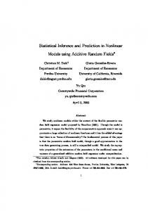
phone subscriptions. The model is estimated using data from the 2012 World Telecommunication Indicators database and covers the period 1990 through 2010 which corresponds to the uptake and diffusion period of mobile cellular use in the US. Figure 2(a) depicts the scatter plots of mobile phone subscriptions over time in the US for the period 1990– 2010 as well as the nonlinear regression fit. As the S-curve theory of new technologies life-cycle predicts, the empirical shape of mobile cellular usage in the US exhibits three

Journal of Probability and Statistics

80

2

60

1

NLS residuals

Subscriptions

8

40

0 −1

20

−2

0 1990

2000 Year

1995

2005

2010

1990

(a)

2000 Year

1995

2005

2010

(b)

Figure 2: Mobile phone subscriptions (per 100 people) and NLS fit (a), NLS residuals plots (b).

stages: incubation, rapid growth, and maturity. The nonlinear regression fit of the data using the Gompertz regression function appears to be graphically satisfactory. The estimation of the model is performed using numerical optimization that requires reasonable start values for the parameters. Unfortunately there are no good rules for starting values except that they should be as insightful as possible so that they are close enough to the final values. Given the growing uptake of the mobile cellular technology, it is reasonable to assume that the number of subscriptions will reach at least 100 per 100 people in the long run. A starting value for the asymptote of around 𝛽10 = 100 is therefore reasonable. If we scale time so that 𝑡 = 0 corresponds to 1990, then substituting 𝛽10 = 100 into the model and using the value 𝑦0 = 2.09 from the data, and assuming that the error is 0, we have 𝛽20 = 3.87. Finally, returning to the data, at time 𝑡 = 1 (i.e., in 1991), the number of subscriptions per 100 people was 𝑦1 = 2.95. Using this value along with previously determined start values and again setting the error to 0 gives 𝛽30 = 0.912. The solution to the optimization problem is then reached after six iterations and an achieved convergence tolerance of 4.227 × 10−6 . Results for the naive nonlinear least squares (NLS) estimation of the model are given in Table 2. The relative growth rate is estimated at 𝛽̂3 = 0.878 and the displacement parameter is estimated at 𝛽̂2 = 4.6. More interestingly, the asymptotic upper bound of the S-curve is estimated at 𝛽̂1 = 131.76; that is, in the long run the number of subscriptions per 100 people would be about 131.8. This implies a relatively high rate of mobile cellular usage compared to the population size. A possible explanation is the absence of Mobile Number Portability (MNP) regulations in the US which could result in subscribers obtaining multiple SIM cards in order to enjoy lower on-net call rates. Figure 2(b) gives the NLS residual plots and Figure 3 plots the autocorrelation function (ACF) and the partial correlation function (PACF) of the residuals. A graphical analysis of the residuals as well as the ACF and PACF plots suggests the presence of first-order positive serial correlation

Table 2: NLS results with errors 𝑢𝑡 ∼ 𝑖𝑖𝑑(0, 𝜎𝑢2 ) and MLE results with MA(1) errors given by (35). Parameters 𝛽1 𝛽2 𝛽3 𝜎𝑢2 𝛾 𝜎𝜖2

Naive NLS estimates Estimates Stand. errors 131.8 4.692 4.600 0.135 0.878 0.005 1.462 0.032 ⋅⋅⋅ ⋅⋅⋅ ⋅⋅⋅ ⋅⋅⋅

ML estimates Estimates Stand. errors 129.3 1.543 4.644 0.021 0.8901 0.001 ⋅⋅⋅ ⋅⋅⋅ 0.709 0.154 1.074 0.004

in the error terms of the model. This intuition can be tested by assuming a first-order moving average structure in the disturbances. To test its significance, assume that the error term 𝑢𝑡 follows the MA(1) process defined by 𝑢𝑡 = 𝜖𝑡 + 𝛾𝜖𝑡−1 ,

with 𝜖𝑡 ∼ 𝑁 (0, 𝜎𝜖2 ) .

(35)

Maximum likelihood (ML) estimates of the model can then be computed by incorporating the above MA(1) errors assumption. The results of the ML estimation are presented in the right panel of Table 2. Using the algorithm described in Section 2 the solution is reached in sixteen iterations after which any further iteration does not substantially change the results. It can be seen that compared to the naive nonlinear least square estimation which does not account for serial correlation the maximum likelihood estimation accounting for MA(1) errors produces different results and smaller standard errors for the estimates. For example, the difference between the NLS estimate for 𝛽3 and its ML estimate is 0.0121 and this difference is significant. The moving average coefficient is estimated at 𝛾̂ = 0.709 with a standard error of 0.154. The achieved convergence tolerance is 8.55 × 10−5 . Based on the MLEs, the 𝑝-value function 𝑝(𝛾) for each of the methods (LR, Wald, and BN) is calculated for hypothesized values of 𝛾 and plotted in Figure 4. They report the results of the test on a more continuous scale so that

Journal of Probability and Statistics

9

ACF

PACF

0.4

NLS residuals

NLS residuals

0.8

0.4

0.0

0.2 0.0 −0.2 −0.4

−0.4 2

0

4

6 Lag

8

10

12

2

4

6

8

10

12

Lag

(a)

(b)

Figure 3: Autocorrelation function (a) and partial autocorrelation function (b) of NLS residuals.

Table 3: Results for 90% and 95% confidence intervals for 𝛾.

1 0.9

Method LR Wald BN

0.8 Probability

0.7 0.6

90% CI for 𝛾 [0.590, 0.934] [0.589, 0.887] [0.587, 0.859]

95% CI for 𝛾 [0.567, 0.978] [0.546, 0.970] [0.509, 0.911]

0.5 0.4

any lag is not significantly different from zero. This further supports the MA(1) model as a plausible error structure for the data.

0.3 0.2 0.1 0 0.4

0.5

Wald LR

0.6 0.7 0.8 Hypothesised values for 𝛾

0.9

1

BN

Figure 4: 𝑝-value function for 𝛾.

any significance level can be chosen for comparison. The two horizontal lines in the figure are the data lines for upper and lower 2.5% levels. Figure 4 shows a clearly distinct pattern between the third-order method (BN) and the firstorder methods (LR and Wald). As an illustration, Table 3 reports the 90% and the 95% confidence interval for 𝛾 from each of the methods. The confidence intervals obtained in Table 3 show considerable differences that could lead to different inferences about 𝛾. The first-order methods, LR and Wald, give wider confidence intervals compared to the confidence intervals produced from the third-order methods, BN. Theoretically, the latter is more accurate. The residuals diagnostics depicted in Figure 5 are also instructive. They show standardized residuals from the ML estimation (a) and the autocorrelation function (ACF) of these residuals (b). All the standardized residuals are within −2 and 2, and the ACF plots show that autocorrelation of

3.3. Empirical Example 2. This empirical example uses a power regression to estimate a general specification of the aggregate consumption function. The example is taken from Greene [27]. The model considered is given by 𝛽

𝐶𝑡 = 𝛽1 + 𝛽2 𝑌𝑡 3 + 𝑢𝑡 ,

𝑡 = 0, 1, . . . , 𝑛,

(36)

where 𝑌𝑡 is personal disposable income and 𝐶𝑡 is aggregate personal consumption. The Keynesian consumption function is a restricted version of this model corresponding to 𝛽3 = 1. With this restriction the model is linear. However, if 𝛽3 is allowed to vary freely, the model is a nonlinear regression. The model is estimated using yearly data from the US economy from 1990 to 2010. As with the preceeding example, estimation requires reasonable start values for the parameters. For the present model, a natural set of values can be obtained because, as we can see, a simple linear regression model is a special case. We can therefore start 𝛽1 and 𝛽2 at their linear least squares values that would correspond to the special case of 𝛽3 = 1 and hence use 1 as a starting value for 𝛽3 . The numerical iterations are therefore started at the linear least squares estimates of 𝛽1 , 𝛽2 , and 1 for 𝛽3 , and convergence is achieved after 8 iterations at a tolerance of 3.111 × 10−6 . Results for the naive linear (OLS) and naive nonlinear least squares (NLS) estimation of the model obtained by assuming 𝑢𝑡 ∼ 𝑖𝑖𝑑(0, 𝜎𝑢2 ), as well as the maximum likelihood

10

Journal of Probability and Statistics

0.8 1 ACF

Standardized MLE residuals

2

0

0.4

0.0 −1 −0.4 1990

2000 Year

1995

2005

2010

0

2

4

(a)

6 Lag

8

10

12

(b)

Figure 5: MLE residuals and their autocorrelation function. 1.0 0.8 1

0.6 ACF

Standardized NLS residuals

2

0

0.4 0.2 0.0

−1

−0.2 −0.4

−2 1990

2000 Year

1995

2005

2010

(a)

0

2

4

6 Lag

8

10

12

(b)

Figure 6: NLS residuals and their autocorrelation function.

estimation obtained by incorporating a first-order moving average for the disturbances as in (35), are given in Table 4. Except for the intercept the estimated nonlinear relationship gives significant estimates from both the proposed and the traditional approaches (see Table 5). In particular, although the power coefficient, 𝛽3 , is numerically close to unity, it is statistically different from one so that the nonlinear specification is a valid alternative with this sample of observations. Moreover, the nonlinear specification has a slightly better explanatory power than the linear specification as the goodness-of-fit is estimated at 0.9998 and 0.9973, respectively. On the other hand, the moving average parameter is estimated at 0.119, very far from the boundary, implying that the likelihood function is likely well-behaved. However, the residuals do not appear to display serial correlation as suggested by Figure 6. In fact, both the firstorder asymptotic test statistics and the proposed third-order procedure fail to reject the null of independence of the disturbances against the MA(1) structure, as evident by the confidence intervals obtained in Table 5. Although in this application all the methods lead to the same conclusion about parameter significance, it is evident

that confidence intervals from the first-order methods (LR and Wald) are nearly indistinguishable while confidence intervals based on third-order method (BN) significantly differ from these intervals.

4. Concluding Remarks In this paper, a third-order likelihood procedure to derive highly accurate 𝑝-values for testing first-order moving average disturbances in nonlinear regression models is illustrated. It is shown how the proposed procedure can also be used to test for MA(1) disturbances in linear regression models and in pure univariate time series models as well. Monte Carlo experiments are used to compare the empirical small sample performance of the proposed third-order method with those of the commonly used first-order methods, particularly, likelihood ratio and Wald departures. Based on the comparison criteria used in the simulations, the results show that the proposed method produces significant improvements over the first-order methods and is superior in terms of central coverage, error probabilities, and average

Journal of Probability and Statistics

11

Table 4: Ordinary least squares, nonlinear least squares, and maximum likelihood with MA(1) errors. Parameters 𝛽1 𝛽2 𝛽3 𝜎𝑢2 𝛾 𝜎𝜖2

OLS estimates Estimates Stand. errors −0.3769 0.0914 0.8606 0.0103 1 ⋅⋅⋅ 0.0140 0.0057 ⋅⋅⋅ ⋅⋅⋅ ⋅⋅⋅ ⋅⋅⋅

NLS estimates Estimates Stand. errors 0.0602 0.6132 0.6986 0.2141 1.067 0.0995 0.0145 0.0065 ⋅⋅⋅ ⋅⋅⋅ ⋅⋅⋅ ⋅⋅⋅

ML estimates Estimates Stand. errors 0.0775 0.0851 0.6925 0.0082 1.0701 0.0019 ⋅⋅⋅ ⋅⋅⋅ 0.1189 0.111 0.0123 0.004

Table 5: Results for 95% confidence intervals for 𝛽1 , 𝛽2 , 𝛽3 , 𝜎2 , and 𝛾. Method LR Wald BN

𝛽1 [−0.087, 0.234] [−0.089, 0.239] [−0.097, 0.138]

𝛽2 [0.672, 0.711] [0.676, 0.708] [0.659, 0.721]

bias. The results suggest that using first-order methods for testing MA(1) disturbances in nonlinear regression models with small samples could be seriously misleading in practice. The implementation of the proposed procedure is illustrated with two empirical examples that use the Gompertz growth model to estimate the diffusion of mobile cellular usage in the US over time and the power regression model to estimate aggregate consumption as a function of disposable income. MATLAB code is available from the author to help with the implementation of this method.

Conflict of Interests The author declares that there is no conflict of interests regarding the publication of this paper.

References [1] P. E. Nguimkeu and M. Rekkas, “Third-order inference for autocorrelation in nonlinear regression models,” Journal of Statistical Planning and Inference, vol. 141, no. 11, pp. 3413–3425, 2011. [2] D. F. Nicholls, A. R. Pagan, and R. D. Terrell, “The estimation and use of models with moving average disturbance terms: a survey,” International Economic Review, vol. 16, pp. 113–134, 1975. [3] P. H. Franses, Time Series Models for Business and Economic Forecasting, Cambridge University Press, Cambridge, Mass, USA, 1998. [4] J. D. Hamilton, Time Series Analysis, Princeton University Press, Princeton, NJ, USA, 1994. [5] H. L¨utkepohl and M. Kratzig, Applied Time Series Econometrics, Cambridge University Press, Cambridge, Mass, USA, 2004.

𝛽3 [1.065, 1.114] [1.066, 1.074] [1.056, 1.072]

𝛾 [−0.095, 0.346] [−0.098, 0.336] [−0.019, 0.249]

𝜎2 [0.006, 0.023] [0.004, 0.021] [0.010, 0.016]

[8] D. A. S. Fraser, N. Reid, and J. Wu, “A simple general formula for tail probabilities for frequentist and Bayesian inference,” Biometrika, vol. 86, no. 2, pp. 249–264, 1999. [9] G. E. P. Box and G. M. Jenkins, Time Series Analysis: Forecasting and Control, Holden-Day, San Francisco, Calif, USA, 1976. [10] A. R. Pagan and D. F. Nicholls, “Exact maximum likelihood estimation of regression models with finite order moving average errors,” Review of Economic Studies, vol. 43, pp. 483– 487, 1976. [11] P. Whittle, Prediction and Regulation by Linear Least-Square Methods, University of Minnesota Press, Minneapolis, Minn, USA, 2nd edition, 1983. [12] J. W. Galbraith and V. Zinde-Walsh, “A simple noniterative estimator for moving average models,” Biometrika, vol. 81, no. 1, pp. 143–155, 1994. [13] J. H. Stock, “Unit roots, structural breaks and trends,” in Handbook of Econometrics, Vol. IV, R. F. Engle and D. L. McFadden, Eds., vol. 2, chapter 46, pp. 2739–2841, NorthHolland, Amsterdam, The Netherlands, 1994. [14] O. E. Barndorff-Nielsen, “Modified signed log likelihood ratio,” Biometrika, vol. 78, no. 3, pp. 557–563, 1991. [15] O. E. Barndorff-Nielsen, “Inference on full and partial parameters based on the standardized signed log-likelihood ratio,” Biometrika, vol. 73, pp. 307–322, 1986. [16] P. Balestra, “A note on the exact transformation associated with the first-order moving average process,” Journal of Econometrics, vol. 14, no. 3, pp. 381–394, 1980. [17] A. Ullah, H. D. Vinod, and R. S. Singh, “Estimation of linear models with moving average disturbances,” Journal of Quantitative Economics, vol. 2, no. 1, pp. 137–152, 1986. [18] D. A. S. Fraser, M. Rekkas, and A. Wong, “Highly accurate likelihood analysis for the seemingly unrelated regression problem,” Journal of Econometrics, vol. 127, no. 1, pp. 17–33, 2005.

[6] D. A. S. Fraser and N. Reid, “Ancillaries and third order significance,” Utilitas Mathematica, vol. 47, pp. 33–53, 1995.

[19] F. Chang and A. C. M. Wong, “Improved likelihood-based inference for the stationary 𝐴𝑅(2) model,” Journal of Statistical Planning and Inference, vol. 140, no. 7, pp. 2099–2110, 2010.

[7] F. Chang, M. Rekkas, and A. Wong, “Improved likelihood-based inference for the MA(1) model,” Journal of Statistical Planning and Inference, vol. 143, no. 1, pp. 209–219, 2013.

[20] A. C. Harvey, “Time series forecasting based on the logistic curve,” Journal of the Operational Research Society, vol. 35, no. 7, pp. 641–646, 1984.

12 [21] D. Fekedulegn, M. P. Mac Siurtain, and J. J. Colbert, “Parameter estimation of nonlinear growth models in forestry,” Silva Fennica, vol. 33, no. 4, pp. 327–336, 1999. [22] P. Young, “Technological growth curves. A competition of forecasting models,” Technological Forecasting and Social Change, vol. 44, no. 4, pp. 375–389, 1993. [23] A. Tsoularis and J. Wallace, “Analysis of logistic growth models,” Mathematical Biosciences, vol. 179, no. 1, pp. 21–55, 2002. [24] P. H. Franses, “Fitting of Gompertz curve,” Journal of the Operational Research Society, vol. 45, no. 1, pp. 109–113, 1994. [25] M. Bengisu and R. Nekhili, “Forecasting emerging technologies with the aid of science and technology databases,” Technological Forecasting and Social Change, vol. 73, no. 7, pp. 835–844, 2006. [26] N. Meade and T. Islam, “Technological forecasting—model selection, model stability, and combining models,” Management Science, vol. 44, no. 8, pp. 1115–1130, 1998. [27] W. H. Greene, Econometric Analysis, Prentice Hall, Englewood Cliffs, NJ, USA, 7th edition, 2012.

Journal of Probability and Statistics

Advances in

Operations Research Hindawi Publishing Corporation http://www.hindawi.com

Volume 2014

Advances in

Decision Sciences Hindawi Publishing Corporation http://www.hindawi.com

Volume 2014

Journal of

Applied Mathematics

Algebra

Hindawi Publishing Corporation http://www.hindawi.com

Hindawi Publishing Corporation http://www.hindawi.com

Volume 2014

Journal of

Probability and Statistics Volume 2014

The Scientific World Journal Hindawi Publishing Corporation http://www.hindawi.com

Hindawi Publishing Corporation http://www.hindawi.com

Volume 2014

International Journal of

Differential Equations Hindawi Publishing Corporation http://www.hindawi.com

Volume 2014

Volume 2014

Submit your manuscripts at http://www.hindawi.com International Journal of

Advances in

Combinatorics Hindawi Publishing Corporation http://www.hindawi.com

Mathematical Physics Hindawi Publishing Corporation http://www.hindawi.com

Volume 2014

Journal of

Complex Analysis Hindawi Publishing Corporation http://www.hindawi.com

Volume 2014

International Journal of Mathematics and Mathematical Sciences

Mathematical Problems in Engineering

Journal of

Mathematics Hindawi Publishing Corporation http://www.hindawi.com

Volume 2014

Hindawi Publishing Corporation http://www.hindawi.com

Volume 2014

Volume 2014

Hindawi Publishing Corporation http://www.hindawi.com

Volume 2014

Discrete Mathematics

Journal of

Volume 2014

Hindawi Publishing Corporation http://www.hindawi.com

Discrete Dynamics in Nature and Society

Journal of

Function Spaces Hindawi Publishing Corporation http://www.hindawi.com

Abstract and Applied Analysis

Volume 2014

Hindawi Publishing Corporation http://www.hindawi.com

Volume 2014

Hindawi Publishing Corporation http://www.hindawi.com

Volume 2014

International Journal of

Journal of

Stochastic Analysis

Optimization

Hindawi Publishing Corporation http://www.hindawi.com

Hindawi Publishing Corporation http://www.hindawi.com

Volume 2014

Volume 2014