May 10, 2006 - that is linear in their code length, and (iii) they have a linear- time bounded-distance decoder. By using a version of the decoder that corrects ...
1
Improved Nearly-MDS Expander Codes
arXiv:cs/0601090v2 [cs.IT] 10 May 2006
Ron M. Roth and Vitaly Skachek
Abstract— A construction of expander codes is presented with the following three properties: (i) the codes lie close to the Singleton bound, (ii) they can be encoded in time complexity that is linear in their code length, and (iii) they have a lineartime bounded-distance decoder. By using a version of the decoder that corrects also erasures, the codes can replace MDS outer codes in concatenated constructions, thus resulting in lineartime encodable and decodable codes that approach the Zyablov bound or the capacity of memoryless channels. The presented construction improves on an earlier result by Guruswami and Indyk in that any rate and relative minimum distance that lies below the Singleton bound is attainable for a significantly smaller alphabet size. Keywords: Concatenated codes, Expander codes, Graph codes, Iterative decoding, Linear-time decoding, Linear-time encoding, MDS codes.
I. I NTRODUCTION
to that of bounded-distance decoding, was then achieved by the authors of this paper in [17], where the iterative decoder of Z´emor was enhanced through a technique akin to generalized minimum distance (GMD) decoding [10], [11]. In [12], Guruswami and Indyk used Z´emor’s construction as a building block and combined it with methods from [1], [3], and [4] to suggest a code construction with the following three properties: (P1) The construction is nearly-MDS: it yields for every designed rate R ∈ (0, 1] and sufficiently small ǫ > 0 an infinite family of codes of rate at least R over an alphabet of size 4 2O((log(1/ǫ))/(Rǫ )) ,
(1)
and the relative minimum distance of the codes is greater than 1−R−ǫ.
In this work, we consider a family of codes that are based on expander graphs. The notion of graph codes was introduced by Tanner in [19]. Later, the explicit constructions of Ramanujan (P2) The construction is linear-time encodable, and the time expander graphs due to Lubotsky, Philips, and Sarnak [8, complexity per symbol is P OLY(1/ǫ) (i.e., this complexChapter 4], [13] and Margulis [15], were used by Alon et ity grows polynomially with 1/ǫ). al. in [1] as building blocks to obtain new polynomial-time (P3) The construction has a linear-time decoder which is constructions of asymptotically good codes in the low-rate essentially a bounded-distance decoder: the correctable range (by “asymptotically good codes” we mean codes whose number of errors is at least a fraction (1−R−ǫ)/2 of rate and relative minimum distance are both bounded away the code length. The time complexity per symbol of the from zero). Expander graphs were used then by Sipser and decoder is also P OLY(1/ǫ). Spielman in [16] to present polynomial-time constructions of In fact, the decoder described by Guruswami and Indyk in [12] asymptotically good codes that can be decoded in time comis more general in that it can handle a combination of errors plexity which is linear in the code length. By combining ideas and erasures. Thus, by using their codes as an outer code in a from [1] and [16], Spielman provided in [18] an asymptotically concatenated construction, one obtains a linear-time encodable good construction where both the decoding and encoding time code that attains the Zyablov bound [9, p. 1949], with a linearcomplexities were linear in the code length. time bounded-distance decoder. Alternatively, such a conWhile the linear-time decoder of the Sipser-Spielman concatenated construction approaches the capacity of any given struction was guaranteed to correct a number of errors that memoryless channel: if the inner code is taken to have the is a positive fraction of the code length, that fraction was smallest decoding error exponent, then the overall decoding significantly smaller than what one could attain by boundederror probability behaves like Forney’s error exponent [10], distance decoding—namely, decoding up to half the mini[11] (the time complexity of searching for the inner code, mum distance of the code. The guaranteed fraction of linearin turn, depends on ǫ, yet not on the overall length of the time correctable errors was substantially improved by Z´emor concatenated code). in [20]. In his analysis, Z´emor considered the special (yet Codes with similar attributes, both with respect to the abundant) case of the Sipser-Spielman construction where Zyablov bound and to the capacity of memoryless channels, the underlying Ramanujan graph is bipartite, and presented were presented also by Barg and Z´emor in a sequence of paa linear-time iterative decoder where the correctable fraction pers [5], [6], [7] (yet in their constructions, only the decoding was 1/4 of the relative minimum distance of the code. An is guaranteed to be linear-time). additional improvement by a factor of two, which brought In this work, we present a family of codes which improves the (linear-time correctable) fraction to be essentially equal on the Guruswami-Indyk construction. Specifically, our codes The authors are with the Computer Science Department, Technion, Haifa will satisfy properties (P1)–(P3), except that the alphabet size 32000, Israel, e-mail: {ronny, vitalys}@cs.technion.ac.il. This work was in property (P1) will now be only supported by the Israel Science Foundation (Grant No. 746/04). Part of this work was presented at the 2004 IEEE Int’l Symposium on Information Theory (ISIT’2004), Chicago, Illinois (June 2004).
3 2O((log(1/ǫ))/ǫ ) .
(2)
2
The basic ingredients of our construction are similar to those used in [12] (and also in [3] and [4]), yet their layout (in particular, the order of application of the various building blocks), and the choice of parameters will be different. Our presentation will be split into two parts. We first describe in Section II a construction that satisfies only the two properties (P1) and (P3) over an alphabet of size (2). These two properties will be proved in Sections III and IV. We also show that the codes studied by Barg and Z´emor in [5] and [7] can be seen as concatenated codes, with our codes serving as the outer codes. The second part of our presentation consists of Section V, where we modify the construction of Section II and use the resulting code as a building block in a second construction, which satisfies property (P2) as well. II. C ONSTRUCTION ′
OF LINEAR - TIME DECODABLE CODES
′′
Let G = (V : V , E) be a bipartite ∆-regular undirected connected graph with a vertex set V = V ′ ∪ V ′′ such that V ′ ∩ V ′′ = ∅, and an edge set E such that every edge in E has one endpoint in V ′ and one endpoint in V ′′ . We denote the size of V ′ by n (clearly, n is also the size of V ′′ ) and we will assume hereafter without any practical loss of generality that n > 1. For every vertex u ∈ V , we denote by E(u) the set of edges that are incident with u. We assume an ordering on V , thereby inducing an ordering on the edges of E(u) for every u ∈ V . For an alphabet F and a word z = (ze )e∈E (whose entries are indexed by E) in F |E| , we denote by (z)E(u) the sub-block of z that is indexed by E(u). Let F be the field GF(q) and let C ′ and C ′′ be linear [∆, r∆, θ∆] and [∆, R∆, δ∆] codes over F , respectively. We define the code C = (G, C ′ : C ′′ ) as the following linear code of length |E| over F : n C = c ∈ F |E| : (c)E(u) ∈ C ′ for every u ∈ V ′ o and (c)E(v) ∈ C ′′ for every v ∈ V ′′
(C is the primary code considered by Barg and Z´emor in [5]). Let Φ be the alphabet F r∆ . Fix some linear one-to-one mapping E : Φ → C ′ over F , and let the mapping ψE : C → Φn be given by � ψE (c) = E −1 ((c)E(u) ) u∈V ′ , c ∈ C . (3)
That is, the entries of ψE (c) are indexed by V ′ , and the entry that is indexed by u ∈ V ′ equals E −1 ((c)E(u) ). We now define the code (C)Φ of length n over Φ by (C)Φ = {ψE (c) : c ∈ C} . Every codeword x = (xu )u∈V ′ of (C)Φ (with entries xu in Φ) is associated with a unique codeword c ∈ C such that E(xu ) = (c)E(u) ,
u∈V′ .
Based on the definition of (C)Φ , the code C can be represented as a concatenated code with an inner code C ′ over F and an outer code (C)Φ over Φ. It is possible, however, to use (C)Φ as an outer code with inner codes other than C ′ . Along these lines, the codes studied in [5] and [7] can be represented as concatenated codes with (C)Φ as an outer code, whereas the inner codes are taken over a sub-field of F .
III. B OUNDS
ON THE CODE PARAMETERS
′
Let C = (G, C : C ′′ ), Φ, and (C)Φ be as defined in Section II. It was shown in [5] that the rate of C is at least r + R − 1. From the fact that C is a concatenated code with an inner code C ′ and an outer code (C)Φ , it follows that the rate of (C)Φ is bounded from below by 1 R r+R−1 =1− + . (4) r r r In particular, the rate approaches R when r → 1. We next turn to computing a lower bound on the relative minimum distance of (C)Φ . By applying this lower bound, we will then verify that (C)Φ satisfies property (P1). Our analysis is based on that in [7], and we obtain here an improvement over a bound that can be inferred from [7]; we will need that improvement to get the reduction of the alphabet size from (1) to (2). We first introduce several notations. Denote by AG the adjacency matrix of G; namely, AG , is a |V | × |V | real symmetric matrix whose rows and columns are indexed by the set V , and for every u, v ∈ V , the entry in AG that is indexed by (u, v) is given by � 1 if {u, v} ∈ E (AG )u,v = . 0 otherwise
It is known that ∆ is the largest eigenvalue of AG . We denote by γG the ratio between the second largest eigenvalue of AG and ∆ (this ratio is less than 1 when G is connected and is nonnegative when n > 1; see [8, Propositions 1.1.2 and 1.1.4]). When G is taken from a sequence of Ramanujan expander graphs with constant degree ∆, such as the LPS graphs in [13], we have √ 2 ∆−1 . γG ≤ ∆ For a nonempty subset S of the vertex set V of G, we will use the notation GS to stand for the subgraph of G that is induced by S: the vertex set of GS is given by S, and its edge set consists of all the edges in G that have each of their endpoints in S. The degree of u in GS , which is the number of adjacent vertices to u in GS , will be denoted by degS (u). Theorem 3.1: The relative minimum distance of the code (C)Φ is bounded from below by p δ − γG δ/θ . 1 − γG In particular, this lower bound approaches δ when γG → 0. The proof of the theorem will make use of Proposition 3.3 below, which is an improvement on Corollary 9.2.5 in Alon and Spencer [2] for bipartite graphs, and is also an improvement on Lemma 4 in Z´emor [20]. We will need the following technical lemma for that proposition. The proof of this lemma can be found in Appendix A. Denote by N (u) the set of vertices that are adjacent to vertex u in G. Lemma 3.2: Let χ be a real function on the vertices of G where the images of χ are restricted to the interval [0, 1]. Write 1 X 1 X χ(u) and τ= χ(v) . σ= n n ′ ′′ u∈V
v∈V
3
Then 1 X X χ(u)χ(v) ∆n ′ u∈V v∈N (u)
p ≤ στ + γG σ(1−σ)τ (1−τ ) √ ≤ (1−γG )στ + γG στ .
(Comparing to the results in [20], Lemma 4 therein is stated for the special case where the images of χ are either 0 or 1. Our first inequality in Lemma 3.2 yields a bound which is always at least as tight as Lemma 4 in [20].) Proposition 3.3: Let S ⊆ V ′ and T ⊆ V ′′ be subsets of sizes |S| = σn and |T | = τ n, respectively, such that σ+τ > 0. Then the sum of the degrees in the graph GS∪T is bounded from above by X √ � degS∪T (u) ≤ 2 (1−γG )στ + γG στ ∆n . u∈S∪T
Proof: We select χ(u) in Lemma 3.2 to be � 1 if u ∈ S ∪ T χ(u) = . 0 otherwise
On the one hand, by Lemma 3.2, X X √ � χ(u)χ(v) ≤ (1−γG )στ + γG στ ∆n . u∈V ′ v∈N (u)
On the other hand, X X X 2 χ(u)χ(v) = degS∪T (u) . u∈V ′ v∈N (u)
u∈S∪T
These two equations yield the desired result. Proof of Theorem 3.1: First, it is easy to see that (C)Φ is a linear subspace over F and, as such, it is an Abelian subgroup of Φn . Thus, the minimum distance of (C)Φ equals the minimum weight (over Φ) of any nonzero codeword of (C)Φ . Pick any nonzero codeword x ∈ (C)Φ , and let c = (ce )e∈E be the unique codeword in C such that x = ψE (c). Denote by Y ⊆ E the support of c (over F ), i.e., Y = {e ∈ E : ce 6= 0} . Let S (respectively, T ) be the set of all vertices in V ′ (respectively, V ′′ ) that are endpoints of edges in Y . In particular, S is the support of the codeword x. Let σ and τ denote the ratios |S|/n and |T |/n, respectively, and consider the subgraph G(Y ) = (S : T, Y ) of G. Since the minimum distance of C ′ is θ∆, the degree in G(Y ) of every vertex in V ′ is at least θ∆. Therefore, the number of edges in G(Y ) satisfies |Y | ≥ θ∆ · σn . Similarly, the degree in G(Y ) of every vertex in V ′′ is at least δ∆ and, thus, |Y | ≥ δ∆ · τ n . Therefore, |Y | ≥ max{θσ, δτ } · ∆n .
On the other hand, G(Y ) is a subgraph of GS∪T ; hence, by Proposition 3.3, √ � 1 X degS∪T (u) ≤ (1−γG )στ + γG στ ∆n . |Y | ≤ 2 u∈S∪T
Combining the last two equations yields
√ max{θσ, δτ } ≤ (1−γG )στ + γG στ .
(5)
We now distinguish between two cases. Case 1: σ/τ ≤ δ/θ. Here (5) becomes √ δτ ≤ (1−γG )στ + γG στ and, so, p p δ − γG δ/θ δ − γG σ/τ ≥ . σ≥ 1 − γG 1 − γG
(6)
Case 2: σ/τ > δ/θ. By exchanging between σ and τ and between θ and δ in (6), we get p θ − γG θ/δ τ≥ . 1 − γG
Therefore,
σ>
p p δ − γG δ/θ δ θ − γG θ/δ δ = . ·τ ≥ · θ θ 1 − γG 1 − γG
Either case yields the desired lower bound on the size, σn, of the support S of x. The next example demonstrates how the parameters of (C)Φ can be tuned so that the improvement (2) of property (P1) holds. Example 3.1: Fix θ = ǫ for some small ǫ ∈ (0, 1] (in which case r > 1−ǫ), and then select q and ∆ so that q > ∆ ≥ 4/ǫ3 . For such parameters, we can take C ′ and C ′′ to be generalized Reed-Solomon (GRS) codes over F . We also assume that G is a Ramanujan bipartite graph, in which case √ 2 ∆−1 < ǫ3/2 . γG ≤ ∆ By (4), the rate of (C)Φ is bounded from below by R 1 + >R−ǫ, 1−ǫ 1−ǫ and by Theorem 3.1, the relative minimum distance is at least p p δ − γG δ/θ 1 ≥ δ − γG δ/θ > δ − ǫ3/2 · √ 1 − γG ǫ = δ − ǫ > 1−R−ǫ . 1−
Thus, the code (C)Φ approaches the Singleton bound when ǫ → 0. In addition, if q and ∆ are selected to be (no larger than) O(1/ǫ3 ), then the alphabet Φ has size 3 |Φ| = q r∆ = 2O((log(1/ǫ))/ǫ ) .
From Example 3.1 we can state the following corollary. Corollary 3.4: For any designed rate R ∈ (0, 1] and sufficiently small ǫ > 0 there is an infinite family of codes (C)Φ of rate at least R and relative minimum distance greater than 1 − R − ǫ, over an alphabet of size as in (2).
4
IV. D ECODING ′
ALGORITHM
′′
Let C = (G, C : C ) be defined over F = GF(q) as in Section II. Figure 1 presents an adaptation of the iterative decoder of Sipser and Spielman [16] and Z´emor [20] to the code (C)Φ , with the additional feature of handling erasures (as well as errors over Φ): as we show in Theorem 4.1 below, the algorithm corrects any pattern of t errors and ρ erasures, provided that t + (ρ/2) < βn, where p (δ/2) − γG δ/θ β= . 1 − γG
Note that β equals approximately half the lower bound in Theorem 3.1. The value of ν in the algorithm, which is specified in Theorem 4.1 below, grows logarithmically with n. We use the notation “?” to stand for an erasure. The algorithm in Figure 1 makes use of a word z = (ze )e∈E over F ∪ {?} that is initialized according to the contents of the received word y as follows. Each sub-block (z)E(u) that corresponds to a non-erased entry y u of y is initialized to the codeword E(y u ) of C ′ . The remaining sub-blocks (z)E(u) are initialized as erased words of length ∆. Iterations i = 3, 5, 7, . . . use an error-correcting decoder D′ : F ∆ → C ′ that recovers correctly any pattern of less than θ∆/2 errors (over F ), and iterations i = 2, 4, 6, . . . use a combined error-erasure decoder D′′ : (F ∪ {?})∆ → C ′′ that recovers correctly any pattern of a errors and b erasures, provided that 2a + b < δ∆ (b will be positive only when i = 2). Theorem 4.1: Suppose that √ θδ > 2γG > 0 , (7) and fix σ to be a positive real number such that p (δ/2) − γG δ/θ σ 0. Let δ be a real number for which the following condition is satisfied for every v ∈ V ′′ : X δ∆ . χ(u) ≥ χ(v) > 0 =⇒ 2 u∈N (v)
Then
r
(δ/2) − (1−γG )σ σ . ≥ τ γG
The proof of Lemma 4.2 can be found in Appendix A. This lemma implies an upper bound on τ , in terms of σ; it can be
verified that this bound is always at least as tight as Lemma 5 in [20]. Proof of Theorem 4.1: For i ≥ 2, let Ui be the value of the set U at the end of iteration i in Figure 1, and let Si be the set of all vertices u ∈ Ui such that (z)E(u) is in error at the end of that iteration. Let χ1 : (V ′ ∪ V ′′ ) → {0, 12 , 1} be the function if u ∈ V ′ and y u is in error 1 1 if u ∈ V ′ and y u is an erasure , χ1 (u) = 2 0 otherwise
and, for i ≥ 2 define the function recursively by 1 0 χi (u) = χi−1 (u) where U1 = V ′ . Denote
σi =
χi : (V ′ ∪ V ′′ ) → {0, 21 , 1} if u ∈ Si if u ∈ Ui \ Si if u ∈ Ui−1
1 X χi (u) . n
,
u∈Ui
Obviously, σ1 n = t + (ρ/2) and, so, by (9) we have σ1 ≤ σ. Let ℓ be the smallest positive integer (possibly ∞) such that σℓ = 0. Since both D′ and D′′ are bounded-distance decoders, a vertex vP∈ Ui can belong to Si for even i ≥ 2, u∈N (v) χi (u) (which equals the sum P only if the sum χ (u)) is at least δ∆/2. Similarly, a vertex v ∈ Ui u∈N (v) i−1 P belongs to Si for odd i > 1, only if u∈N (v) χi (u) ≥ θ∆/2. It follows that the function χi satisfies the conditions of Lemma 4.2 (with θ taken instead of δ for odd i) and, so, δ 1−γG r − σi−1 for even 0 < i < ℓ σi−1 2γ γG G ≥ . σi θ − 1−γG σi−1 for odd 1 < i < ℓ 2γG γG (10) Using the condition σ1 ≤ σ < β, it can be verified by induction on i ≥ 2 that � σi−1 δ/θ for even 0 < i < ℓ ≥ . (11) θ/δ for odd 1 < i < ℓ σi Hence, for every i > 2, σi−2 σi−1 δ θ σi−2 = · ≥ · =1; σi σi−1 σi θ δ in particular, σi ≤ σ for odd i and σi ≤ σ2 for even i. Incorporating these inequalities into (10) yields 1 δ 1−γG √ σ for even 0 < i < ℓ − √ ≥ √ σi 2γG σi−1 γG (12) and θ 1−γG √ 1 for odd 1 < i < ℓ . − σ2 √ ≥ √ σi 2γG σi−1 γG (13) By combining (12) and (13) we get that for even i > 0, 2γG 2(1−γG ) √ 1 + σ2 ≥ √ √ θ σi+1 θ σi δ 1−γG √ ≥ − σ, √ 2γG σi−1 γG
5
n ′ in (Φ ∪ {?}) . Received word y = (y u )u∈V � E (y u ) if y u ∈ Φ Initialize: For u ∈ V ′ do: (z)E(u) ← . ?? . . . ? if y u = ? Iterate: For i = 2, 3, . . . , ν do: (a) If i is odd then U ≡ V ′ and D ≡ D′ , else U ≡ V ′′ and D ≡ D′′ . (b) For every u ∈ U do: (z)E(u) ← D ((z)E(u) ). Output: ψE (z) if z ∈ C (and declare ‘error’ otherwise).
Input:
Fig. 1.
Decoder for (C)Φ .
or 1 √ σi+1
≥ ≥ =
� � √ θδ 1−γG θ σ √ − + σ2 √ 4γG2 σi−1 γG 2γG r ! 1−γG θ θδ θ √ − + σ √ 4γG2 σi−1 γG 2γG δ � √ � √ 1 θδ σ σ + − , (14) √ 2 4γG σi−1 β β
where the second inequality follows from σ2 ≤ σ · θ/δ (see (11)), and the (last) equality follows from the next chain of equalities: r ! 1−γG θ θ √ σ + γG 2γG δ r √ � σθ 1−γG � 2γG + θδ = 2γG2 δ r 2 1−γG 4γG − θδ σθ = − ·√ 2γG2 δ θδ − 2γG � � √ (1−γG ) σ θδ p = − 1− 2 4γG (δ/2) − γG δ/θ �√ � θδ σ . = − 1− 2 4γG β Consider the following first-order linear recurring sequence (Λj )j≥0 that satisfies � √ � √ θδ σ σ Λ − + Λj+1 = , j≥0, j 2 4γG β β √ √ where Λ0 = 1/ σ. From (14) we have 1/ σi+1 ≥ Λi/2 for even i ≥ 0. By solving the recurrence for (Λj ), we obtain ! �i/2 � � � σ σ 1 1 θδ √ . (15) 1− + ≥ Λi/2 = √ σi+1 4γG2 β β σ From the condition (7) we thus get that σi+1 decreases exponentially with (even) i. A sufficient condition for ending the decoding correctly after ν iterations is having σν < 1/n, or √ 1 √ > n. σν We require therefore that ν be such that ! �(ν−1)/2 � � � √ σ σ 1 θδ 1 √ > n. 1− + √ ≥ 2 4γG β β σ σν
The latter inequality can be rewritten as �(ν−1)/2 � √ √ β nσ − σ θδ nσ − (σ/β) > = , 4γG2 1 − (σ/β) β−σ thus yielding
� � √ β nσ − σ +1, ν > 2 log β−σ
where the base of the logarithm equals (θδ)/(4γG2 ). In summary, the decoding will end with the correct codeword after $ � √ �% β nσ − σ ν = 2 log +3 β−σ iterations (where the base of the logarithm again equals (θδ)/(4γG2 ).) In Lemma B.1, which appears in Appendix B, it is shown that the number of actual applications of the decoders D′ and D′′ in the algorithm in Figure 1 can be bounded from above by ω · n, where � √ � ∆β σ θ log 1+ β−σ δ � � ω = 2· � 2 �2 . + θδ 4γG log 1− 4γG2 θδ
Thus, if θ and δ are fixed and the ratio σ/β is bounded away from 1 and G is a Ramanujan graph, then the value of ω is bounded from above by an absolute constant (independent of ∆). The algorithm in Figure 1 allows us to use GMD decoding in cases where (C)Φ is used as an outer code in a concatenated code. In such a concatenated code, the size of the inner code is |Φ| and, thus, it does not grow with the length n of (C)Φ . A GMD decoder will apply the algorithm in Figure 1 a number of times that is proportional to the minimum distance of the inner code. Thus, if the inner code has rate that is bounded away from zero, then the GMD decoder will have time complexity that grows linearly with the overall code length. Furthermore, if C ′ , C ′′ , and the inner code are codes that have a polynomial-time bounded-distance decoder—e.g., if they are GRS codes—then the multiplying constant in the linear expression of the time complexity (when measured in operations in F ) is P OLY(∆). For the choice of parameters in Example 3.1, this constant is P OLY (1/ǫ) and, since F is chosen in that example to have size O(1/ǫ3 ), each operation in F can in turn be implemented by P OLY(log(1/ǫ)) bit
6
operations. (We remark that in all our complexity estimates, we assume that the graph G is “hard-wired” so that we can ignore the complexity of figuring out the set of incident edges of a given vertex in G. Along these lines, we assume that each access to an entry takes constant time, even though the length of the index of that entry may grow logarithmically with the code length. See the discussion in [16, Section II].) When the inner code is taken as C ′ , the concatenation results in the code C = (G, C ′ : C ′′ ) (of length ∆n) over F , and the (linear-time) correctable fraction of errors is then the product θ · σ, for any positive real σ that satisfies (8). A special case of this result, for F = GF(2) and C ′ = C ′′ , was presented in our earlier work [17], yet the analysis therein was different. A linear-time decoder for C was also presented by Barg and Z´emor in [7], except that their decoder requires finding a codeword that minimizes some weighted distance function, and we are unaware of a method that performs this task in time complexity that is P OLY(∆)—even when C ′ and C ′′ have a polynomial-time bounded-distance decoder. V. C ONSTRUCTION
WHICH IS ALSO LINEAR - TIME
ENCODABLE
In this section, we use the construction (C)Φ of Section II as a building block in obtaining a second construction, which satisfies all properties (P1)–(P3) over an alphabet whose size is given by (2).
Let C = (G, C ′ : C ′′ ) be defined over F = GF(q) as in Section II. The first simple observation that provides the intuition behind the upcoming construction is that the encoding of C, and hence of (C)Φ , can be easily implemented in linear time if the code C ′ has rate r = 1, in which case Φ = F ∆ . The definition of C then reduces to o n C = c ∈ F |E| : (c)E(v) ∈ C ′′ for every v ∈ V ′′ .
We can implement an encoder of C as follows. Let E ′′ : F R∆ → C ′′ be some one-to-one encoding mapping of C ′′ . Given an information word η in F R∆n , it is first recast into a word of length n over F R∆ by sub-dividing it into sub-blocks η v ∈ F R∆ that are indexed by v ∈ V ′′ ; then a codeword c ∈ C is computed by v ∈ V ′′ .
By selecting E in (3) as the identity mapping, we get that the respective codeword x = (xu )u∈V ′ = ψE (c) in (C)Φ is xu = (c)E(u) ,
Fix now a list of vectors s = (hu )u∈V ′ where hu ∈ F (1−r0 )∆ , and define the subset C(s) of C by C(s) = {c ∈ C : (c)E(u) ∈ C0 (hu ) for every u ∈ V ′ } ; accordingly, define the subset (C(s))Φ of (C)Φ by n o (C(s))Φ = ψE (c) = ((c)E(u) )u∈V ′ : c ∈ C(s) .
Now, if s is all-zero, then C(s) coincides with the code C(0) = (G, C0 : C ′′ ); otherwise, C(s) is either empty or is a coset of C(0), where C(0) is regarded as a linear subspace of C over F . From this observation we conclude that the lower bound in Theorem 3.1 applies to any nonempty subset (C(s))Φ , except that we need to replace θ by θ0 . In addition, a simple modification in the algorithm in Figure 1 adapts it to decode (C(s))Φ so that Theorem 4.1 holds (again under the change θ ↔ θ0 ): during odd iterations i, we apply to each sub-block (z)E(u) a bounded-distance decoder of C0 (hu ), instead of the decoder D′ . Therefore, our strategy in designing the linear-time encodable codes will be as follows. The raw data will first be encoded into a codeword c of C (where C ′ = Φ). Then we compute the n vectors hu = H0 · (c)E(u) ,
A. Outline of the construction
(c)E(v) = E ′′ (η v ) ,
h ∈ F (1−r0 )∆ , denote by C0 (h) the following coset of C0 within Φ: C0 (h) = {v ∈ Φ : H0 v = h} .
u∈V′ .
Thus, each of the ∆ entries (over F ) of the sub-block xu can be associated with a vertex v ∈ N (u), and the value assigned to that entry is equal to one of the entries in E ′′ (η v ). While having C ′ = Φ (= F ∆ ) allows easy encoding, the minimum distance of the resulting code (C)Φ is obviously poor. To resolve this problem, we insert into the construction another linear [∆, r0 ∆, θ0 ∆] code C0 over F . Let H0 be some ((1−r0 )∆) × ∆ parity-check matrix of C0 and for a vector
u∈ V′ ,
and produce the list s = (hu )u∈V ′ ; clearly, c belongs to C(s). The list s will then undergo additional encoding stages, and the result will be merged with ψE (c) to produce the final codeword. The parameters of C0 , which determine the size of s, will be chosen so that the overhead due to s will be negligible. During decoding, s will be recovered first, and then we will apply the aforementioned adaptation to (C(s))Φ of the decoder in Figure 1, to reconstruct the information word η. B. Details of the construction We now describe the construction in more detail. We let F be the field GF(q) and ∆1 and ∆2 be positive integers. The construction makes use of two bipartite regular graphs, G1 = (V ′ : V ′′ , E1 )
and
G2 = (V ′ : V ′′ , E2 ) ,
of degrees ∆1 and ∆2 , respectively. Both graphs have the same number of vertices; in fact, we are making a stronger assumption whereby both graphs are defined over the same set of vertices. We denote by n the size of V ′ (or V ′′ ) and by Φ1 and Φ2 the alphabets F ∆1 and F ∆2 , respectively. The notations E1 (u) and E2 (u) will stand for the sets of edges that are incident with a vertex u in G1 and G2 , respectively. We also assume that we have at our disposal the following four codes: • a linear [∆1 , r0 ∆1 , θ0 ∆1 ] code C0 over F ; • a linear [∆1 , R1 ∆1 , δ1 ∆1 ] code C1 over F ; • a linear [∆2 , R2 ∆2 , δ2 ∆2 ] code C2 over F ;
7
a code Cm of length n and rate rm over the alphabet Φm = F R2 ∆2 . The rates of these codes need to satisfy the relation •
(1−r0 )∆1 = rm R2 ∆2 , and the code Cm is assumed to have the following properties: 1) Its rate is bounded away from zero: there is a universal positive constant κ such that rm ≥ κ. 2) Cm is linear-time encodable, and the encoding time per symbol is P OLY(log |Φm |). 3) Cm has a decoder that recovers in linear-time any pattern of up to µn errors (over the alphabet Φm ), where µ is a universal positive constant. The time complexity per symbol of the decoder is P OLY(log |Φm |). (By a universal constant we mean a value that does not depend on any other parameter, not even on the size of Φm .) For example, we can select as Cm the code of Spielman in [18], in which case κ can be taken as 1/4. Based on these ingredients, we introduce the codes C1 = (G1 , Φ1 : C1 )
and
C2 = (G2 , Φ2 : C2 )
over F . The code C1 will play the role of the code C as outlined in Section V-A, whereas the codes Cm and C2 will be utilized for the encoding of the list s that was described there. The overall construction, which we denote by C, is now defined as the set of all words of length n over the alphabet Φ = Φ1 × Φ2 that are obtained by applying the encoding algorithm in Figure 2 to information words η of length n over F R1 ∆1 . A schematic diagram of the algorithm is shown in Figure 3. (In this algorithm, we use a notational convention whereby entries of information words η are indexed by V ′′ , and so are codewords of Cm .) From the discussion in Section V-A and from the assumption on the code Cm it readily follows that the encoder in Figure 2 can be implemented in linear time, where the encoding complexity per symbol (when measured in operations in F ) is P OLY(∆1 , ∆2 ). The rate of C is also easy to compute: the encoder in Figure 2 maps, in a one-to-one manner, an information word of length n over an alphabet of size q R1 ∆1 , into a codeword of length n over an alphabet Φ of size q ∆1 +∆2 . Thus, the rate of C is R1 R1 ∆1 n = . (16) (∆1 + ∆2 )n 1 + (∆2 /∆1 ) In the next section, we show how the parameters of C can be selected so that it becomes nearly-MDS and also linear-time decodable. C. Design, decoding, and analysis We will select the parameters of C quite similarly to Example 3.1. We assume that the rates R1 and R2 of C1 and C2 are the same and are equal to some prescribed value R, and define αR = 8 · (1−R) · max{R/µ, 2/κ}
(notice that αR can be bounded from above by a universal constant that does not depend on R, e.g., by 16/ min{2µ, κ}). We set θ0 = κ · ǫ for some positive ǫ < R (in which case 1−r0 < κ · ǫ), and then select q, ∆1 , and ∆2 so that q > ∆1 ≥ αR /ǫ3 and ∆2 =
(1−r0 )∆1 rm R
(< ∆1 ) ;
(17)
yet we also assume that q is (no larger than) O(1/ǫ3 ). The graphs G1 and G2 are taken as Ramanujan graphs and C0 , C1 , and C2 are taken as GRS codes over F . (Requiring that both ∆1 and ∆2 be valid degrees of Ramanujan graphs imposes some restrictions on the value (1−r0 )/(rm R). These restrictions can be satisfied by tuning the precise rate of Cm last.) Given this choice of parameters, we obtain from (17) that ∆2 /∆1 < ǫ/R and, so, the rate (16) of C is greater than R >R−ǫ. 1 + (ǫ/R)
(18)
The alphabet size of C is 3 |Φ| = |Φ1 | · |Φ2 | = q ∆1 +∆2 = 2O((log(1/ǫ))/ǫ ) ,
as in (2), where we have absorbed into the O(·) term the constants κ and µ. Our next step in the analysis of the code C consists of showing that there exists a linear-time decoder which recovers correctly any pattern of t errors and ρ erasures, provided that 2t + ρ ≤ (1−R−ǫ)n .
(19)
This, in turn, will also imply that the relative minimum distance of C is greater than 1−R−ǫ, thus establishing with (18) the fact that C is nearly-MDS. Let x = (xu )u∈V ′ be the transmitted codeword of C, where xu = ((c)E1 (u) , (d)E2 (u) ) , and let y = (y u )u∈V ′ be the received word; each entry y u takes the form (y u,1 , y u,2 ), where y u,1 ∈ Φ1 ∪{?} and y u,2 ∈ Φ2 ∪{?}. Consider the application of the algorithm in Figure 4 to y, assuming that y contains t errors and ρ erasures, where 2t + ρ ≤ (1−R−ǫ)n. Step (D1) is the counterpart of the initialization step in Figure 1 (the entries of z here are indexed by the edges of G2 ). ˜ ∈ Φnm that The role of Step (D2) is to compute a word w is close to the codeword w of Cm , which was generated in Step (E3) of Figure 2. Step (D2) uses the inverse of the encoder E2 (which was used in Step (E4)) and also a combined errorerasure decoder D2 : (F ∪{?})∆2 → C2 that recovers correctly any pattern of a errors (over F ) and b erasures, provided that 2a + b < δ2 ∆2 . The next lemma provides an upper bound on ˜ (as words of length the Hamming distance between w and w n over Φm ). Lemma 5.1: Under the assumption (19), the Hamming dis˜ (as words over Φm ) is less than µn. tance between w and w
8
Input: Information word η = (η v )v∈V ′′ of length n over F R1 ∆1 . (E1)
Using an encoder E1 : F R1 ∆1 → C1 , map η into a codeword c of C1 by (c)E1 (v) ← E1 (η v ) ,
(E2)
v ∈ V ′′ .
Fix some ((1−r0 )∆1 ) × ∆1 parity-check matrix H0 of C0 over F , and compute the n vectors u∈V′ ,
hu ← H0 · (c)E1 (u) , to produce the list s = (hu )u∈V ′ . (E3) (E4)
Regard s as a word of length (1−r0 )∆1 n (= rm R2 ∆2 n) over F , and map it by an encoder of Cm into a codeword w = (w v )v∈V ′′ of Cm . Using an encoder E2 : F R2 ∆2 → C2 , map w into a codeword d of C2 by (d)E2 (v) ← E2 (w v ) ,
v ∈ V ′′ .
Output: Word x = (xu )u∈V ′ in (Φ1 × Φ2 )n whose components are given by the pairs xu = ((c)E1 (u) , (d)E2 (u) ) , Fig. 2.
Encoder for C.
Step (E1)
Step (E2)
Step (E3)
Graph G1
- E1 - E1 - E1 - E1 - E1 r r r
ηv
- E1 - E1
�� � tH t H0 � JH � � @ �� �H� �� J@ �H - H0 H t� t H J@ �� @HJ �� �� �@ H �� @ � H t� �J @ - H0 Ht J� @ �@� �� � @ �� � J � @ - H0 Jt �� @ � @ tH s Encoder ��
�H� H� @ �� �� H of Cm t� � - H0 Ht @ H � H � �� r r r r r r (c)E1 (u) E1 (η v ) hu �� � � H t� Ht - H0 � H� � H �� �� �H �� �H @ H @t - H0 t� ��
Information word η
Fig. 3.
u∈V′ .
Schematic diagram of the encoder for C.
-
Step (E4) �
Graph G2
- E2 - E2 w - �
wv
Codeword x
tH �t JH � � @ �H� J@ �H t� �t H J@ �H @HJ �� �@ H � �JH@ t�@ Ht J� @ �@� ���@J @ Jt �� @ � @ tH � H � � H@ t� � H@ � Ht H � H � r r r (d)E (u) E2 (w v ) � 2 � H � t� Ht H� � H �� �H �H @ H @t t�
- E2 -
- E2 - E2 r r r
- E2 - E2 �
9
Input: Received word y = (y u )u∈V ′ in (Φ ∪ {?})n . � y u,2 if y u,2 ∈ Φ1 (D1) For u ∈ V ′ do: (z)E2 (u) ← . ?? . . . ? if y u,2 = ? For v ∈ V ′′ do:
(D2)
˜ v ← E2−1 (D2 ((z)E2 (v) )). w
ˆ ∈ F (1−r0 )∆1 n . ˜ = (w ˜ v )v∈V ′′ to produce an information word s Apply a decoder of Cm to w
(D3)
Apply a decoder for (C1 (ˆ s))Φ1 to (y u,1 )u∈V ′ , as described in Section V-A, to produce an information word ˆ = (ˆ η η v )v∈V ′′ .
(D4)
ˆ = (ˆ Output: Information word η η v )v∈V ′′ of length n over F R∆1 . Fig. 4.
Decoder for (C)Φ .
Proof: Define the 1 1 2 χ(u) = 1 0
function χ : (V ′ ∪ V ′′ ) → {0, 12 , 1} by if u ∈ V ′ and y u,2 is in error if u ∈ V ′ and y u,2 is an erasure ˜ u 6= wu if u ∈ V ′′ and w otherwise
.
˜ 6= w, this function satisfies the conditions Assuming that w of Lemma 4.2 with respect to the graph G2 , where σn equals t + (ρ/2) and τ n equals the number of vertices v ∈ V ′′ such ˜ v 6= wv . By that lemma we get that w r (δ2 /2) − σ (δ2 /2) − (1−γ2 )σ σ ≥ ≥ τ γ2 γ2 1−R − 2σ ǫ > ≥ , (20) 2γ2 2γ2 where γ2 stands for γG2 and the last inequality follows from (19). Now, by (17) we have ∆2 =
and, so, by (19), the conditions of Theorem 4.1 hold for σ = √ (1−R−ǫ)/2 (note that β > 0 yields θ0 δ1 > 2γ1 , thus (7) holds).
(1−r0 )∆1 8(1−R) ǫ∆1 αR ≥ , > ≥ rm R R R · ǫ2 µ · ǫ2
from which we get the following upper bound on the square of γ2 : 4(∆2 −1) 4 µ · ǫ2 γ22 ≤ < ≤ . 2 ∆2 ∆2 2(1−R) Combining this bound with (20) yields 1−R σ > , τ 2µ namely, τ < 2µσ/(1−R) < µ. It follows from Lemma 5.1 that Step (D2) reduces the ˜ to the extent that allows a linear-time number of errors in w ˜ in Step (D3). decoder of Cm to fully recover the errors in w ˆ, which is computed in Step (D3), is identical Hence, the list s with the list s that was originally encoded in Step (E2). Finally, to show that Step (D4) yields complete recovery from errors, we apply Theorem 4.1 to the parameters of the code (G1 , C0 : C1 ). Here θ0 = κ · ǫ and 2ǫ3/2 ǫ3/2 2 ; ≤ √ ≤ p γ1 = γG1 < √ αR ∆1 2 (1−R)/κ
therefore,
p r (δ1 /2) − γ1 δ1 /θ0 1−R 1−R 1−R−ǫ β= > > − γ1 1 − γ1 2 θ0 2
A PPENDIX A We provide here the proofs of Lemmas 3.2 and 4.2. Given a bipartite graph G = (V ′ : V ′′ , E), we associate with G a |V ′ | × |V ′′ | real matrix XG whose rows and columns are indexed by V ′ and V ′′ , respectively, and (XG )u,v = 1 if and only if {u, v} ∈ E. With a proper ordering on V ′ ∪ V ′′ , the matrix XG is related to the adjacency matrix of G by XG 0 . AG = (21) XGT 0 Lemma A.1: Let G = (V ′ : V ′′ , E) be a bipartite ∆-regular graph where |V ′ | > 1. Then ∆2 is the largest eigenvalue of the (symmetric) matrix XGT XG and the all-one vector 1 is a corresponding eigenvector. The second largest eigenvalue of XGT XG is γG2 ∆2 . Proof: We compute the square of AG , 0 XG XGT 2 , AG = 0 XGT XG
and recall the following two known facts: (i) XG XGT and XGT XG have the same set of eigenvalues, each with the same multiplicity [14, Theorem 16.2]. (ii) If λ is an eigenvalue of AG , then so is −λ, with the same multiplicity [8, Proposition 1.1.4]. We conclude that λ is an eigenvalue of AG if and only if λ2 is an eigenvalue XGT XG ; furthermore, when λ 6= 0, both these eigenvalues have the same multiplicities in their respective matrices. The result readily follows. For real column vectors x, y ∈ Rm p, let hx, yi be the scalar product xT y and kxk be the norm hx, xi. Lemma A.2: Let G = (V ′ : V ′′ , E) be a bipartite ∆-regular graph where |V ′ | = n > 1 and let s = (su )u∈V ′ and t = (tu )u∈V ′′ be two column vectors in Rn . Denote by σ and τ the averages 1 X 1 X σ= su and τ= tu , n n ′ ′′ u∈V
u∈V
10
and let the column vectors y and z in Rn be given by y = s−σ·1
z = t−τ ·1.
and
Define the vector x ∈ R
where E′G {χi } =
1 X (χ(u)i ) , n ′
E′′G {χi } =
1 X (χ(u)i ) , n ′′
2n
by � � s x= . t
u∈V
Var′G {χ} = E′G {χ2 } − (E′G {χ})2 ,
Then, and
|hx, AG xi − 2στ ∆n| ≤ 2γG ∆kyk · kzk .
Var′′G {χ} = E′′G {χ2 } − (E′′G {χ})2 .
Proof: First, it is easy to see that XG 1 = XGT 1 = ∆ · 1 and that hy, 1i = hz, 1i = 0; these equalities, in turn, yield the relationship: hy, XG zi = hs, XG ti − στ ∆n .
Proof: Define the column vectors s = (χ(u))u∈V ′ , and x=
Secondly, from (21) we get that hx, AG xi = 2hs, XG ti . Hence, the lemma will be proved once we show that |hy, XG zi| ≤ γG ∆kyk · kzk .
(22)
�
t = (χ(u))u∈V ′′ , s t
�
,
and denote by σ and τ the averages 1 X 1 X su and τ= tu . σ= n n ′ ′′ u∈V
u∈V
The following equalities are easily verified:
Let λ1 ≥ λ2 ≥ . . . ≥ λn
EG {w} =
XGT XG
be the eigenvalues of and let v 1 , v 2 , . . . , v n be corresponding orthonormal eigenvectors where, by Lemma A.1, √ λ1 = ∆2 , λ2 = γG2 ∆2 , and v 1 = (1/ n) · 1 . Write z=
n X
√ where βi = hz, v i i. Recall, however, that β1 = (1/ n) · hz, 1i = 0; so, = = ≤
hz, XGT XG zi n n n DX E X X βi v i , λi βi v i = λi βi2 kv i k2 i=2 n X
λ2
i=2
βi2
i=2
i=2
2
= λ2 kzk =
γG2 ∆2 kzk2
Lemma A.3: Let G = (V ′ : V ′′ , E) be a bipartite ∆-regular graph where |V ′ | = n > 1 and let χ : (V ′ ∪ V ′′ ) → R be a function on the vertices of G. Define the function w : E → R and the average EG {w} by w(e) = χ(u)χ(v)
for every edge e = {u, v} in G
and EG {w} =
1 · ks − σ · 1k2 , n
Var′′G {χ} =
1 · kt − τ · 1k2 . n
The result now follows from Lemma A.2. Proof of Lemma 3.2: Using the notation of Lemma A.3, write 1 X X χ(u)χ(v) , (23) EG {w} = ∆n ′ u∈V v∈N (u)
.
The desired result (22) is now obtained from the CauchySchwartz inequality.
1 X w(e) . ∆n e∈E
Then q ′ ′′ EG {w} − E′G {χ} · E′′G {χ} ≤ γG VarG {χ} · VarG {χ} ,
E′′G {χ} = τ ,
Var′G {χ} = and
βi v i ,
hx, AG xi , 2∆n
E′G {χ} = σ ,
i=1
kXG zk2
u∈V
E′G {χ} =
1 X χ(u) = σ , n ′
E′′G {χ} =
1 X χ(u) = τ . n ′′
and
(24)
u∈V
(25)
u∈V
Since the range of χ is restricted to the interval [0, 1], we have E′G {χ2 } ≤ E′G {χ}
and
E′′G {χ2 } ≤ E′′G {χ} ;
hence, the values Var′G {χ} and Var′′G {χ} can be bounded from above by Var′G {χ} ≤ σ − σ 2
and
Var′′G {χ} ≤ τ − τ 2 . (26)
Substituting (23)–(26) into Lemma A.3 yields 1 �X X � p χ(u)χ(v) − στ ≤ γG σ(1−σ)τ (1−τ ) ; ∆n ′ u∈V v∈N (u)
11
so, 1 X X χ(u)χ(v) ∆n u∈V ′ v∈N (u) p ≤ στ + γG σ(1−σ)τ (1−τ ) � p √ �√ = (1−γG )στ + γG στ στ + (1−σ)(1−τ ) √ ≤ (1−γG )στ + γG στ , as claimed. Proof of Lemma 4.2: We compute lower and upper bounds on the average 1 X X χ(u)χ(v) . ∆n ′′ v∈V
u∈N (v)
On the one hand, this average equals X 1 δ∆ X δτ 1 X χ(u) ≥ χ(v) χ(v) = · , ∆n ∆n 2 2 u∈N (v) v∈V ′′ : v∈V ′′ | {z } | {z } χ(v)>0 τn
≥δ∆/2
where the inequality follows from the assumed conditions on χ. On the other hand, this average also equals √ 1 X X χ(u)χ(v) ≤ (1−γG )στ + γG στ , ∆n ′ u∈V v∈N (u)
where the inequality follows from Lemma 3.2. Combining these two bounds we get √ δτ ≤ (1−γG )στ + γG στ , 2 and the result is now obtained by dividing by γG τ and rearranging terms. A PPENDIX B When analyzing the complexity of the algorithm in Figure 1, one can notice that the decoder D ∈ {D′ , D′′ } needs to be applied at vertex u, only if (z)E(u) has been modified since the last application of D at that vertex. Based on this observation, we prove the following lemma. Lemma B.1: The number of (actual) applications of the decoders D′ and D′′ in the algorithm in Figure 1 can be bounded from above by ω · n, where � √ � ∆β σ θ 1+ log β − σ δ � + � ω =2· � 2 �2 . 4γG log θδ 1− 4γG2 θδ Proof: Define iT by
iT
√ � ∆β σ log β − σ � � = 2· . log θδ 4γG2
�
It is easy to verify that � �i /2 � √ � θδ T σ 1 √ ≥ ∆. − 4γG2 β σ
(27)
In the first iT iterations in Figure 1, we apply the decoder D (which is either D′ or D′′ ) at most iT · n times. Next, we evaluate the total number of applications of the decoder D in iterations i = iT + 1, iT + 2, · · · , ν. We hereafter use the notations Ui and Si as in the proof of Theorem 4.1. Recall that we need to apply the decoder D to (z)E(u) for a vertex u ∈ Ui+2 , only if at least one entry in (z)E(u) — say, the one that is indexed by the edge {u, v} ∈ E(u) — has been altered during iteration i + 1. Such an alteration may occur only if v is a vertex in Ui+1 with an adjacent vertex in Si . We conclude that D needs to be applied at vertex u during iteration i + 2 only if u ∈ N (N (Si )). The number of such vertices u, in turn, is at most ∆2 |Si | = ∆2 · σi n. We now sum the values of ∆2 σi n over iterations i = iT + 1, iT + 2, · · · , ν: ∆2 n ·
ν X
σi
i=iT +1
=
≤
∆2 n 2
∆ n·
⌊(ν−2)/2⌋
⌊(ν−1)/2⌋
X
σ2j+1 +
X
j=iT /2
j=iT /2
⌊(ν−1)/2⌋
� � θ σ2j+1 1 + , δ
X
j=iT /2
σ2j+2 (28)
where the last inequality is due to (11). From (15) (and by neglecting a positive term), we obtain �i/2 � � √ � 1 θδ 1 σ √ − ≥ √ σi+1 4γG2 σ β for even i ≥ iT . Therefore, the expression in (28) is bounded from above by � � � 2 �iT 4γG θ 2 ∆ n 1+ · δ θδ � 2 �2 ! � √ �2 4γG σ 1 √ − 1− θδ σ β � � 1 θ · 2 ∆2 n 1 + δ ∆ ≤ � 2 �2 4γG 1− θδ � � θ n 1+ δ = � 2 �2 , 4γG 1− θδ where the inequality follows from (27). Adding now the number of applications of the decoder D during the first iT iterations, we conclude that the total number of applications of the decoder D is at most ω · n, where θ 1+ δ ω = iT + � 2 �2 . 4γG 1− θδ
12
R EFERENCES [1] N. Alon, J. Bruck, J. Naor, M. Naor, and R.M. Roth, “Construction of asymptotically good low-rate error-correcting codes through pseudorandom graphs,” IEEE Trans. Inf. Theory, vol. 38, no. 2, pp. 509–516, Mar. 1992. [2] N. Alon and J.H. Spencer, The Probabilistic Method, 2nd ed. New York: Wiley, 2000. [3] N. Alon, J. Edmonds, and M. Luby, “Linear time erasure codes with nearly optimal recovery,” in Proc. 36th Annual IEEE Symp. on Foundations of Computer Science (FOCS), Milwaukee, Wisconsin, Oct. 1995, pp. 512–519. [4] N. Alon and M. Luby, “A linear time erasure-resilient code with nearly optimal recovery,” IEEE Trans. Inf. Theory, vol. 42, no. 6, pp. 1732– 1736, Nov. 1996. [5] A. Barg and G. Z´emor, “Error exponents of expander codes,” IEEE Trans. Inf. Theory, vol. 48, no. 6, pp. 1725–1729, June 2002. [6] A. Barg and G. Z´emor, “Error exponents of expander codes under linearcomplexity decoding,” SIAM J. Discrete Math., vol. 17, no. 3, pp. 426– 445, 2004. [7] A. Barg and G. Z´emor, “Concatenated codes: serial and parallel,” IEEE Trans. Inf. Theory., vol. 51, no. 5, pp. 1625–1634, May 2005. [8] G. Davidoff, P. Sarnak, and A. Valette, Elementary Number Theory, Group Theory, and Ramanujan Graphs. Cambridge, UK: Cambridge University Press, 2003. [9] I. Dumer, “Concatenated codes and their multilevel generalizations,” in Handbook of Coding Theory, Volume II, V.S. Pless and W.C. Huffman (Editors), Amsterdam, Netherlands: North-Holland, pp. 1911–1988, 1998. [10] G.D. Forney, Jr., Concatenated Codes. Cambridge, Massachusetts: MIT Press, 1966. [11] G.D. Forney, Jr., “Generalized minimum distance decoding,” IEEE Trans. Inf. Theory, vol. 12, no. 2, pp. 125–131, Apr. 1966. [12] V. Guruswami and P. Indyk, “Near-optimal linear-time codes for unique decoding and new list-decodable codes over smaller alphabets,” in Proc. 34th Annual ACM Symposium on Theory of Computing (STOC), Montr´eal, Quebec, Canada, pp. 812–821, May 2002. [13] A. Lubotsky, R. Philips, and P. Sarnak, “Ramanujan graphs,” Combinatorica, vol. 8, pp. 261–277, 1988. [14] C.C. MacDuffee, The Theory of Matrices. New York: Chelsea, 1946. [15] G.A. Margulis, “Explicit group theoretical constructions of combinatorial schemes and their applications to the design of expanders and concentrators,” Probl. Inf. Transm., vol. 24, no. 1, pp. 39–46, July 1988. [16] M. Sipser and D.A. Spielman, “Expander codes,” IEEE Trans. Inf. Theory, vol. 42, no. 6, pp. 1710–1722, Nov. 1996. [17] V. Skachek and R.M. Roth, “Generalized minimum distance iterative decoding of expander codes,” in Proc. IEEE Inf. Theory Workshop (ITW), Paris, France, pp. 245–248, Mar.-Apr. 2003. [18] D.A. Spielman, “Linear-time encodable and decodable error-correcting codes,” IEEE Trans. Inf. Theory, vol. 42, no. 6, pp. 1723–1731, Nov. 1996. [19] R.M. Tanner, “A recursive approach to low-complexity codes,” IEEE Trans. Inf. Theory, vol. 27, no. 5, pp. 533–547, Sep. 1981. [20] G. Z´emor, “On expander codes,” IEEE Trans. Inf. Theory, vol. 47, no. 2, pp. 835–837, Feb. 2001.