Improved Passive Splitting Keith D. Cooper Jason Eckhardt∗ Department of Computer Science Rice University Houston, TX, U.S.A. Abstract— We present a graph coloring register allocator which uses an improved form of passive live range splitting to reduce the count of dynamic spill operations. Program structure is used to guide the global splitting of live ranges and to place split operations at infrequently executed portions of the program. We also optimistically reconsider spill decisions at certain points to potentially enable more splits and/or fewer spills. Certain issues that complicate implementation of the original passive splitting method are discussed. Finally, experimental results are presented which indicate that the improved passive splitter is effective. Keywords— global register allocation, live range splitting.
1 I NTRODUCTION The Chaitin-Briggs (“CB”) graph coloring register allocation framework [7], [6], [3], [2], [4] is generally regarded as the dominant paradigm for global register allocation in optimizing compilers. The technique is highly effective, but its method of spilling live ranges— sometimes referred to informally as the “spill everywhere” approach— may insert far more spill operations than necessary. A number of approaches have been proposed for improving on the limitations of the CB spill method [1], [5], [11], [9], [10]. One general way of attacking the problem is by live range splitting— breaking certain live ranges into smaller pieces so that each piece can be allocated independently. Such splitting may enable a graph to be colored with fewer colors, or allow more intelligent placement of spill instructions. In [2], Briggs describes an aggressive approach to splitting. In this method live ranges are split before the coloring phase by the insertion of split operations (copies) at certain points in the program. For example, splits can be inserted at the boundaries of loops for global live ranges that span the loop. For a live range x, this allows the allocator to consider the portion of x within the loop separately from the portion outside the loop. Briggs attempted a number of ways of choosing split points, such as by using loop boundaries, dominator frontiers, etc. The technique is considered aggressive in that every range live at a split point would be split. While the experiments showed significant wins for the strategy, it also showed significant losses due to excessive split copies remaining in the code. In an effort to obtain some of the benefits of splitting, while not incurring as many losses as aggressive splitting, Cooper and Simpson introduced a lazy or passive approach [8]. Their results indicate that a less aggressive approach can still significantly reduce dynamic spill operations compared to the standard Chaitin-Briggs allocator, without incurring the big ∗ Correspondence:
Jason Eckhardt (
[email protected])
losses of being too aggressive. This paper introduces some modifications that boost the effectiveness of passive splitting. Section 2 provides an overview of the original passive splitting allocator. Section 3 discusses opportunities for improvement and presents a modified version of the algorithm. Experimental results for the new technique are given in Section 4. Finally, Section 5 discusses some other implementation issues. 2 C HAITIN -B RIGGS A LLOCATOR W ITH PASSIVE S PLITTING Passive splitting (“PS”) was designed to cope with some of the situations in which Chaitin’s “spill everywhere” approach performs poorly. Figure 1a portrays one such case. Suppose for the sake of illustration that the allocator has only one register available. Since there are two conflicting live ranges x and y, CB will completely spill one or the other. Assuming y is chosen for spilling, a store of y will be inserted after every definition and a load before every use, producing the code in Figure 1b. Unfortunately, this approach leads to a new load operation that will execute on each iteration of the loop. Simpson observed that this undesirable situation can be avoided by splitting x around y. That is, because x is not used until the second loop, it need not occupy a register until after the first loop (after y dies). This allows y to occupy the register during its lifetime in the first loop. By splitting in this fashion, spill operations are placed outside of either of the loops, and both live ranges occupy a register in the frequently executed portions of their lifetimes, as shown in Figure 1c. The key to Simpson’s approach is solidifying the notion of when one live range can be split around another. In the example, splitting was allowed because y is contained in x— all the uses and definitions of y occur entirely between any uses or definitions of x. 2.1 Overview of the Algorithm Passive splitting is implemented with a small number of changes to the overall CB framework, as depicted in Figure 2. Items in boldface represent phases that were changed or added to CB. In addition the the interference graph used by CB, Simpson builds a containment graph which indicates the containment relationships between any pair of live ranges. The graph is built using an algorithm nearly identical to that for building an interference graph. It is the data structure used during splitting to determine whether or not a split is feasible. The graph is
spill code split code
renumber
build
coalesce
spill costs
simplify
select
split costs
find splits
Fig. 2.
The Passive Splitting Allocator
x=... y=...
x=... y=... store y
x=... store x y=...
...=y
load y ...=y
...=y
load x
...=x
...=x
...=x
for spilling as usual. 3. Find splits: Invoked by select, this is the key routine that determines whether splitting can free a color for a node n that did not receive a color. Utilizing the containment graph and the computed split costs, it will try to either split interfering live ranges around n, or split n around interfering live ranges, choosing the least costly choice. Further, the choice is only acceptable if it costs less than spilling n everywhere. 4. Split code: Once a split decision has been made, the actual instructions must be inserted into the code. This operates similarly to the spill code phase of CB. For each live range s that was split around l, a STORE of s is inserted before every definition of l, and a LOAD of s is inserted after every death of l. 3 S OME I MPROVEMENTS
(a)
(b)
(c)
Fig. 1. Example of passive splitting: (a) original; (b) spill y completely; (c) split x around y.
actually built at the beginning of the split costs phase described below. It was not mentioned in Simpson’s original paper, but a special phase is run before register allocation to remove all critical edges in the control flow graph. This is done to ensure that there is always a proper location in which to place split operations. 1. Split costs: For each live range l, this phase determines the cost of splitting a live range s around l, where the cost is the number of LOAD and STORE instructions (weighted by loop nesting depth) needed to perform the split. The underlying implementation operates similarly to the spill costs phase in CB. 2. Select: This phase operates as in CB, with one change. When a node n is encountered that cannot receive a color, find splits is called in an attempt to find a color for n by splitting. If splitting was successful, n will now be assigned a color and is no longer marked for spilling. If splitting was not successful, n is marked
Simpson reports good results for passive splitting, and experiments by this author confirm that PS can significantly reduce dynamic spill operations compared to CB. Even so, examination of some benchmarks reveals that even better results are achievable. Consider the code in Figure 3a. Suppose that during select node t did not receive a color, and that find splits determines that splitting x around t is less costly than spilling t everywhere.1 Recall that split code will insert a STORE before every definition of t and a LOAD after every death of t. In this example, that has the unfortunate drawback of placing all the split instructions within the loop (Figure 3b). But by observing that x has no reference (use or definition) within the first loop, a much better placement for the split operations is just outside the loop (Figure 3c). That is, the dynamic number of spill operations will be decreased because the split code is placed in less frequently executed regions of the program. In the case of a deeply nested loop, the splits can be pushed outside of more than one loop in the nest as long as there are no references to the split range in that loop. Using loops to guide the splitting is convenient in that it is relatively easy to differentiate high frequency regions from 1 The
split is legal since x contains t.
x=... store x
is feasible (he, ci ∈ / CG), it is more costly than just spilling e, since c is at a greater loop depth. Thus, e is marked for spilling. Continuing, a is popped and assigned color 2, the only possibility. Finally, b is popped but cannot receive a color. store x t=... t=... t=......=t ...=t ...=t This time, however, find splits determines that a split of ...=t d around b is both legal (hd, bi ∈ / CG) and less costly than ...=t ...=t load x spilling b. Thus the split is noted and b is assigned color 1. At this point, the stack is empty, and once spill and split code is inserted, the next phase of allocation will build and color load x the resulting graph successfully (i.e., without introducing any more splits or spills). Rather than accepting the spill of e as just described, an examination of the live ranges just after the spill and split code ... ... ... is inserted (Figure 4c) reveals that we can do better. Suppose ... ... ... that instead of marking e for spilling, it is reconsidered for allocation in the next pass. This time e is a candidate for (a) (b) (c) splitting around the second part of d (the range starting at the Fig. 3. Example of improved passive splitting: (a) original; (b) split x around load of d). Not only that, doing the split is less costly than t (old); (c) split x around t (new). spilling e. The previous example shows that splitting enabled a node d= d= store d that was destined for spilling to be allocated to a register— b= a= b= a= d c =a =a but only because it was reconsidered rather than spilled in the e= e= =e first pass. In other words, instead of pessimistically spilling =e =b =b e =b b all nodes that were marked for spilling we optimistically =b load d c= c= assume that splitting (if any) has enabled one or more of them =c =c a to become colorable. This seemingly simple modification to =d =d =e select makes a significant difference on the benchmarks =e =e =e used here. x=...
(a)
x=...
(b)
(c)
Fig. 4. Spill reconsideration opportunity (k = 2): (a) live ranges; (b) containment graph CG; (c) live ranges after first pass (e in memory)
those of low frequency with purely static control flow analysis. Unless a loop has a tiny trip count (e.g., one), or the body of the loop is guarded by a rarely true condition, then it is a fairly safe to assume that moving split code out of a loop is better when possible. It is also possible to use other program structure to guide the splitting, such as with conditional regions. However, unlike loops, it is not necessarily obvious by static analysis which part of a conditional executes more frequently than the other. By incorporating profile feedback from a training run, the allocator could decide how to place split code in or around conditionals. The allocator framework used in the present work does not currently use profiling feedback. Another opportunity for improvement arises in select. Consider the live ranges depicted in Figure 4a. Suppose that the number of colors is k = 2 ({1,2}), the coloring stack created by simplify is d, c, e, a, b (d is the stack top), and that only c is in a loop. Now during select, d is popped off the coloring stack first and assigned color 1. Next c is popped and assigned color 2. When e is popped, it cannot be assigned a color since all colors are used by neighbors d and c. At this point, find splits attempts to free a color by considering a split of e around c. While the split
3.1 The Improved Algorithm Figure 5 depicts the improved passive allocator, with changes from the original marked in boldface. A detailed explanation of the new functionality is given next. The implementation was performed in the Rice Scalar Compiler Group’s ILOC compiler, starting with the original passive splitting code written by Simpson. 3.1.1 Build Loop Tree In order to make use of loops when computing spill costs and inserting split code, the new phase build loop tree constructs a convenient representation of the program. This data structure, the LoopTree, represents the hierarchical loop nesting structure of the program.2 Each node in the LoopTree represents a loop. A node c is a child of node p if the loop represented by c is contained within the loop represented by p, and c is contained in no other loops. If two disjoint loops have the same containing loop, then they will be sibling nodes with the same parent node. Each node t also contains the following: t.blocks is a list of all the basic blocks contained in this loop, but not any of its inner loops; t.parent points to the parent node; t.depth is the loop nesting depth (depth 1 is an outermost loop). The actual control flow analysis method used here to determine loops is based on DJ-graphs [12], though a number of other techniques would work as well. This pass is performed once before the main register allocation starts. 2 To simplify this discussion, it is assumed that all loops are reducible. However, reducibility is not a requirement for the algorithm.
spill code split code (w/ loops)
renumber
build
coalesce
spill costs
simplify
split costs (w/ loops)
build loop tree
find splits
Fig. 5.
The Improved Passive Splitting Allocator
annotateLoopTree(t) t.refs ← {} t.spilled on entry[*] ← {} t.reloaded on exit[*] ← {} For each inner loop c of t annotateLoopTree(c) t.refs ← t.refs ∪ c.refs For each block b in t.blocks For each instruction i in b For each live range l defined in i t.refs ← t.refs ∪ l For each live range l used in i t.refs ← t.refs ∪ l Fig. 6.
select (reconsider spills)
Algorithm for loop annotation
3.1.2 Split Costs Before starting, split costs needs to annotate the LoopTree with additional information about virtual register usage within the loops. This information will be queried to determine the legality of pushing a split out of a loop or loops. Figure 6 shows the annotation algorithm. The algorithm computes (or initializes) three additional sets of information for each loop. Member t.refs is the set of all virtual registers referenced (used or defined) in the subtree rooted at t. Set t.spilled on entry[e] contains the name of each VR that has previously been spilled to memory on edge e before the loop is entered. Likewise, set t.reloaded on exit[e] contains the name of each VR that has previously been reloaded from memory on edge e after the loop is exited. The algorithm will perform a postorder (bottom-up) traversal of the loop tree, propagating information up the tree. For each loop, all ranges which have have a reference in the current loop t are added to t.refs. After each subtree of t has been processed, its’ ref set is incorporated into the current set for t. Simpson’s original method of performing splitting is based on the idea that for every live range si split across live range l, si will be stored immediately before a definition of l, and reloaded just after a death of l. Thus, for some si , the same split code will be inserted around l as any other sj (except,
splitCosts() buildContainmentGraph() annotateLoopTree(LoopTree.root) For each block b live ← liveOutb For each successor s of b deaths ← liveOutb −liveIns For each m ∈ deaths calcPerNeighborCosts(m, s, ForDeath) For each inst i in b in reverse order For each live range l defined in i calcPerNeighborCosts(l, b, ForDef) For each live range l used in i if l ∈ / live calcPerNeighborCosts(l, b, ForDeath) Update the live set calcPerNeighborCosts(l, b, type) deflt weight ← 10depth(b) For each neighbor n of l / containment graph if hn, li ∈ pushout ← 0 p ← loop(b) while p 6= NIL ∧ n ∈ / p.refs pushout ← pushout + 1 new weight ← 10p.depth−1 p ← p.parent if pushout > 0 weight = new weight else weight = deflt weight if type = ForDef l.split costs[n].stores ← l.split costs[n].stores + weight else if type = ForDeath l.split costs[n].loads ← l.split costs[n].loads + weight Fig. 7.
Algorithm for computing split costs
select() ··· while ¬coloring stack.empty ··· c ← pick color for name if c = invalid color spillset ← spillset ∪ name if findSplits(name) = TRUE spillset ← spillset − name if pass number = 1 spillset ← {} ··· Fig. 8.
Algorithm fragment for color selection
of course, the name). To represent split costs then, a single quantity was stored with each live range l. That quantity being the cost of splitting any si around l. The key to the new approach is realizing that it can be beneficial to split si around l in a different way than splitting sj around l. For example, a death of l may occur within a loop, while a splittable neighbor si has no references in the loop. At the same time, another splittable neighbor sj has a reference in the loop. For the former case, it is desirable to insert the split operations for si outside the loop, while a reload of sj would be required (as originally) just after the death of l. To model the previous scenario, a single cost stored with l is no longer sufficient. Instead, costs are stored for every neighbor n of l, and split costs will compute a distinct cost for splitting n around l. Figure 7 shows the new method of computing costs. For every basic block in the compilation unit, split costs iterates through the instructions in reverse order and maintains a set live of currently live ranges. If either a definition or death of l is detected in the current instruction, then every neighbor of l is examined to determine a split cost for that neighbor. There are currently two options. Either the split cost will be based on the default location (i.e., just before the definition of l or just after the death of l), or the loop tree will be consulted to determine whether the split cost can be decreased by pushing the split operation out of a loop. To determine whether pushing splittable neighbor s out is possible, the algorithm traverses the loop tree in a bottom-up fashion. It first obtains the loop tree node pi containing l, then iteratively checks whether s has any references in pi and then moves to the parent loop pi−1 . If pi−1 contains a reference of s, then the iteration stops and pi is the outermost loop that s can be pushed out of. 3.1.3 Select As described earlier, it can be beneficial to reconsider spill decisions after splitting. Thus, at the end of select (Figure 8), the spill set is cleared if any splits were made. This is done only on the first build-color pass, in order to minimize compile-time impact. The rationale being that most splitting will happen on the first pass, and allowing reconsideration on every pass has diminishing returns. However, it may
still be worthwhile to provide a command line option to allow reconsideration on every pass. 3.1.4 Find Splits This phase operates very similarly to the original passive splitter, except that when considering the neighbors n of l, it must utilize the new per-neighbor cost for each n. In Figure 9, symbols RC, SC, and LC are constants that represent machine-dependent costs for rematerialization instructions, store instructions, and load instructions respectively. 3.1.5 Split Code As seen in Figures 10 and 11, the highlevel operation of split code is similar to split costs. That is, definitions and deaths of a live range l are detected on a reverse pass through the instructions in a basic block. This time, however, the actual split instructions are inserted into the program. For a live range s split around l, if no pushing out is possible, then a LOAD of s is inserted into the instruction stream just after a death of l and a STORE of s just before any definitions of l. In either case, if a split range s can be rematerialized, then no STORE of s is necessary and LOADs are replaced with cheaper LOAD-IMMEDIATEs. For splits which can be pushed out of a loop, code insertion is slightly more complicated. Placing a split operation “just outside” a loop L means either placing it on an edge entering L from outside of L (loop entry edges), or placing it on an edge exiting to a block outside of L (loop exit edges). Since it is assumed that all critical edges have been split before register allocation, there is always a place to insert such operations— in the block at the head (tail) of an entry (exit) edge. Consider the case in which s is split around m in loop L and the STORE of s is pushed out of L. Function placeSplit iterates over every loop entry edge e of L, checking if s is live on edge e. Range s is live on edge e if s ∈ (liveOute.pred ∩ liveIne.succ ). Only the liveOute.pred set actually needs to be checked, though, since s is known to be live throughout L (it has no references in L yet it interferes with m). If s is live on e, then the STORE of s is inserted at the end of basic block e.pred (the block at the head of e). Similar processing happens when a LOAD is pushed out of L. This time, however, the operation will be placed on the exit edges of L where it is live. Liveness on an exit edge e is checked by examining liveIne.succ . Any time an operation for s is placed outside a loop L on edge e, s is added to either the set L.spilled on entry[e] or L.reloaded on exit[e]. Since s may have been split across more than one range, the processing above would normally insert a split operation at the loop boundary for every live range s was split around. Such redundant operations are suppressed by checking whether s has already been spilled (or reloaded) around L. 4 E XPERIMENTS To test the effectiveness of the passive splitting improvements, we compared Simpson’s original splitter to the new splitter, both of which are implemented
findSplits(l) bestCost ← range[l].cost splitFound ← FALSE For each color c /* Try to split c around l. */ splitOK ← TRUE cost ← 0 For each neighbor n of l with colors[n] = c if hn, li ∈ containment graph splitOK ← FALSE else if rematerializable(n) cost ← cost + l.split costs[n].loads × RC else cost ← cost + l.split costs[n].stores × SC + l.split costs[n].loads × LC if splitOK ∧ cost < bestCost bestCost ← cost bestColor ← c splitDir ← splitAroundName splitFound ← TRUE /* Try to split l around c. */ splitOK ← TRUE cost ← 0 For each neighbor n of l with colors[n] = c if hl, ni ∈ containment graph splitOK ← FALSE else if rematerializable(l) cost ← cost + n.split costs[l].loads × RC else cost ← cost + n.split costs[l].stores × SC + n.split costs[l].loads × LC if splitOK ∧ cost < bestCost bestCost ← cost bestColor ← c splitDir ← splitAroundColor splitFound ← TRUE if splitFound = TRUE colors[l] ← bestColor if splitDir = splitAroundName For each neighbor n of l with colors[n] = bestColor Mark n to be split around l else For each neighbor n of l with colors[n] = bestColor Mark l to be split around n Fig. 9.
Algorithm for determining splits
splitCode() For each block b live ← liveOutb For each successor s of b deaths ← liveOutb −liveIns For each m ∈ deaths For each live range l split around m placeSplit(l, s, s.firstinst, ForDeath) For each inst i in b in reverse order For each live range l defined in i For each live range s split around l if ¬rematerializable(s) placeSplit(s, b, i, ForDef) For each live range l used in i if l ∈ / live For each live range s split around l placeSplit(s, b, i.nextinst, ForDeath) Update the live set Fig. 10.
Algorithm for inserting split code
in the ILOC compiler. The compiler first runs the original program through a series of optimization passes, and gives the result to the register allocator for processing. The optimization flags used were -r[-RD]v[-vfsmp]zc[-mf]dv[-vfsmp]zc[-f]dn, which causes these passes to run (in order, with repetition): reassociation, value numbering, lazy code motion, constant propagation, dead code elimination, value numbering, lazy code motion, constant propagation, dead code elimination, and control flow clean-up. Simpson’s original study benchmarked program wave5 (SPEC95). We chose the same program and also added tomcatv (SPEC92), and g271decoder (MediaBench). The first three columns of Table 1 show the number of dynamic spill operations executed by each allocator, where each row represents one procedure from a benchmark program. All procedures which executed any spill operations were included in the table. The remaining columns show the percentage improvement (where percent improvement is calculated as old−new × 100). In the table headings P S denotes the original old passive splitter, P S ∗ is the new splitter (program structure only), and P S ∗∗ is the new splitter with both program structure and spill reconsideration. Adding program structure decreased the dynamic spill operation count in 11 of the 25 procedures, in some cases dramatically. Improvements ranged from 0.08% all the way up to 50% for denpt. Two procedures show small losses while 12 procedures showed no change. By using both program structure and spill reconsideration, 14 procedures improved, with three routines showing better than 49% reduction in spill overhead. The few losses that occurred relative to P S can happen for two reasons— the same reasons mentioned by Simpson regarding P S compared to Chaitin-Briggs without splitting.
placeSplit(n, b, deflt inst, type) pushout ← 0 t ← NIL p ← loop(b) while p 6= NIL ∧ n ∈ / p.refs pushout ← pushout + 1 t←p p ← p.parent if type = ForDef if pushout > 0 For each entry edge e of loop t pred ← e.pred if n ∈ liveOutpred ∧ n ∈ / t.spilled on entry[e] t.spilled on entry[e] ← t.spilled on entry[e] ∪ n Insert STORE n at end of pred else if pushout = 0 Insert STORE n before deflt inst in b else if type = ForDeath if pushout > 0 For each exit edge e of loop t succ ← e.succ if n ∈ liveInsucc ∧ n ∈ / t.reloaded on exit[e] t.reloaded on exit[e] ← t.reloaded on exit[e] ∪ n if rematerializable(n) Insert a LOAD-IMMEDIATE for n at beginning of succ else Insert LOAD of n at beginning of succ else if pushout = 0 if rematerializable(n) Insert a LOAD-IMMEDIATE of n before deflt inst in b else Insert LOAD of n before deflt inst in b Fig. 11.
Algorithm for placing split code
First, all spill and split cost analysis is currently done with static estimates. These estimates cannot predict actual runtime behavior with perfect accuracy, so that spills or splits might be placed in unfortunate locations. Second, after a round of splitting/spilling, the second pass of allocation will be presented with a different interference graph. This means that simplify might make completely different decisions than it did in the first pass. Improved passive splitting has a reasonable compile time cost, as shown in Table 2. P S ∗ increases compile time between 4 and 6% over P S, while P S ∗∗ increases it by 6 to 17%. Most of the extra time spent in P S ∗∗ is due the the extra renumber-build-color cycle needed when spills are reconsidered. 5 OTHER I SSUES AND M ODIFICATIONS As specified in Simpson’s original article, the passive splitting algorithm is unable to function correctly for certain
TABLE 1 DYNAMIC SPILL OPERATIONS FOR wave5, g271decoder, tomcatv (25 INTEGER /25 FLOAT REGISTERS , 13/13, AND 14/14 RESPECTIVELY ) Proc. celbnd denpt energy fftb fftf field getb init injchk numb parmvr pdiag putb radb2 radb4 radb5 radf2 radf4 radf5 rffti1 slv2xy smooth vslv1p update main
PS 880 2700002 200216 125275 125275 13494690 820728 504020 10 16 6518815 93792 59597 3724700 7292900 5414900 3756000 7731100 5414900 32 900 8062200 11934370 19847517 52483505
P S∗ 720 1350002 200216 125275 125275 13243885 812912 504020 10 16 6826430 93792 58620 3505600 7105100 5414900 3756000 7480700 5414900 32 925 6937280 11903095 19847517 52442514
P S ∗∗ 720 1350002 100696 125275 125275 13309290 789440 505870 10 16 6831315 93792 57643 3536900 6948600 5414900 3536900 7292900 5414900 32 825 6562180 12117520 10031360 49831213
% P S∗ 18.18 50.00 0 0 0 1.86 0.95 0 0 0 -4.72 0 1.64 5.88 2.58 0 0 3.24 0 0 -2.78 13.95 0.26 0 0.08
% P S ∗∗ 18.18 50.00 49.70 0 0 1.37 3.81 -0.37 0 0 -4.79 0 3.28 5.04 4.72 0 5.83 5.67 0 0 8.33 18.61 -1.53 49.46 5.05
TABLE 2 C OMPILE - TIME IMPACT OF IMPROVED PASSIVE SPLITTING ( SECONDS ) Benchmark wave5 g271decode tomcatv
PS 54 0.84 0.48
P S∗ 56 0.89 0.50
P S ∗∗ 62 0.89 0.56
P S∗ PS
P S ∗∗ PS
1.04 1.06 1.04
1.15 1.06 1.17
kinds of instruction-set architectures or compiler intermediate representations. None of these issues affect the ILOC compiler used for the original implementation, which is somewhat simplified compared to other compilers. Also, ILOC itself is generally simpler and cleaner than many actual machine instruction sets. However, it is likely that industrial practioners or other researchers using different compiler infrastructures will be impacted. 5.1 Representing Call-clobbered Registers at Call Sites In some compilers, the clobbering of caller-saved registers at a call site is represented by adding extra operands to a procedure call instruction (one for each register clobbered). Each new operand is marked as a definition of the corresponding register. Under this scenario, split costs and split code will not operate properly if they try to split a range around one of these definitions. That is, the definition will signal that a STORE is needed, but since it has no later uses, no LOAD operation (to reload the split range) will be signalled. A small modification is made so that while processing a definition of a range that is not already live, it is treated like a death. That is, a LOAD will be needed after the definition and the cost must be adjusted accordingly. The situation must be detected while processing definitions because the defined
register has no use in any instruction, so that it will have never become live, and hence never seen by the code dealing with deaths. For example, in calcPerNeighborCosts, two lines are added to the “ForDef” case as shown below. An analogous, but slightly more complicated change is needed in placeSplits as well.
calcPerNeighborCosts(l, b, type) ··· if type = ForDef l.split costs[n].stores ← l.split costs[n].stores + weight if l ∈ / live l.split costs[n].loads ← l.split costs[n].loads + weight ··· 5.2 Two-address Instructions/Modified Input Operands Many existing (and entrenched) instruction set architectures contain two-address instructions or other instructions that both read and write a register operand. For example, both the PowerPC and PA-RISC ISAs have load and store instructions that update the index register. For the Intel x86 series, most arithmetic instructions are two-address, overwriting one of the two inputs with the result. Such instructions present a real complication for the original splitting algorithm. Consider the following fragment in Intel x86-like psuedo-assembly code (using virtual register numbers).
VR1 = · · · VR2 = · · · ··· ADD VR2,[EBP+32] ··· · · · = VR2 ··· · · · = VR1 Suppose P S decides to split VR1 around VR2. Where should it insert the store operations? Normally, that would be done at every definition of VR2 but clearly that presents a problem here. The idea behind splitting VR1 is to use the same register for it that VR2 has been assigned. The second inserted store of VR1 (before the ADD instruction) would store the improper value, since it would have been overwritten by the first write of VR2 (recall, they both will share the same physical register). Therefore, the reload back into VR1, which would be placed after the last use of VR2 would get the wrong value. Because the ADD both reads VR2 for its data, and writes VR2 with its result, we cannot view the write of VR2 as a new live range. In essence, the register mentioned in a modified input must be treated as a single live range. A solution has been implemented, but we do not have space to present the details here. 6 C ONCLUSIONS AND F UTURE W ORK Simpson’s passive splitting is an elegant extension to Chaitin-Briggs that successfully attacks the “spill everywhere”
problem. We presented algorithmic improvements that increase its effectiveness even more (up to 50% fewer dynamic spill operations) by incorporating program structure directly into the splitting process and by reconsidering spill decisions. The improved algorithm also maintains the elegance and simplicity of the original, so that practitioners can consider including the method into their Chaitin-Briggs-style allocators. Future work includes incorporating conditional program structure into the allocator, along with the profile feedback necessary to support it. It would be interesting to re-implement the algorithm in a production-quality compiler targeted to a mainstream microprocessor architecture. This would also permit a much wider range of applications to be tested. ACKNOWLEDGEMENTS Tim Harvey answered numerous questions about the ILOC compiler and the original passive splitting implementation. R EFERENCES [1] Peter Bergner, Peter Dahl, David Engebretsen, and Matthew T. O’Keefe. Spill Code Minimization via Interference Region Spilling. In SIGPLAN Conference on Programming Language Design and Implementation, pages 287–295, 1997. [2] Preston Briggs. Register Allocation via Graph Coloring. Technical Report TR92-183, Rice University, 24, 1992. [3] Preston Briggs, Keith D. Cooper, and Linda Torczon. Rematerialization. In Proceedings of the Conference on Programming Language Design and Implementation (PLDI), volume 27, pages 311–321, New York, NY, 1992. ACM Press. [4] Preston Briggs, Keith D. Cooper, and Linda Torczon. Improvements to Graph Coloring Register Allocation. ACM Transactions on Programming Languages and Systems, 16(3):428–455, May 1994. [5] D. Callahan and B. Koblenz. Register Allocation via Hierarchical Graph Coloring. SIGPLAN, 26(6):192–203, June 1991. [6] G.J. Chaitin. Register Allocation and Spilling via Graph Coloring. In SIGPLAN82, 1982. [7] G.J. Chaitin, M.A. Auslander, A.K. Chandra, J. Cocke, M.E. Hopkins, and P.W. Markstein. Register Allocation via Coloring. Computer Languages, 6:45–57, January 1981. [8] K. D. Cooper and L.T. Simpson. Live range Splitting in a Graph Coloring Register Allocator. In Proceedings of the International Compiler Construction Conference, March 1998. [9] Kathleen Knobe and Kenneth Zadeck. Register Allocation Using Control Trees. Technical Report CS-92-13, Brown University, Department of Computer Science, March 1992. [10] Guei-Yuan Lueh, Thomas Gross, and Ali-Reza Adl-Tabatabai. Fusionbased register allocation. ACM Transactions on Programming Languages and Systems, 22(3):431–470, 2000. [11] Cindy Norris and Lori L. Pollock. Register Allocation over the Program Dependence Graph. In SIGPLAN Conference on Programming Language Design and Implementation, pages 266–277, 1994. [12] Vugranam C. Sreedhar, Guang R. Gao, and Yong-Fong Lee. Identifying loops using dj graphs. ACM Transactions on Programming Languages and Systems, 18(6):649–658, 1996.