Improved Query Performance with Variant Indexes - Duke Computer ...

Improved Query Performance with Variant Indexes Patrick O’Neil

Dallan Quass

Department of Mathematics and Computer Science University of Massachusetts at Boston Boston, MA 02125-3393 [email protected]

Department of Computer Science Stanford University Stanford, CA 94305 [email protected]

Abstract: The read-mostly environment of data warehousing makes it possible to use more complex indexes to speed up queries than in situations where concurrent updates are present. The current paper presents a short review of current indexing technology, including row-set representation by Bitmaps, and then introduces two approaches we call Bit-Sliced indexing and Projection indexing. A Projection index materializes all values of a column in RID order, and a Bit-Sliced index essentially takes an orthogonal bit-by-bit view of the same data. While some of these concepts started with the MODEL 204 product, and both Bit-Sliced and Projection indexing are now fully realized in Sybase IQ, this is the first rigorous examination of such indexing capabilities in the literature. We compare algorithms that become feasible with these variant index types against algorithms using more conventional indexes. The analysis demonstrates important performance advantages for variant indexes in some types of SQL aggregation, predicate evaluation, and grouping. The paper concludes by introducing a new method whereby multi-dimensional group-by queries, reminiscent of OLAP/Datacube queries but with more flexibility, can be very efficiently performed. 1. Introduction Data warehouses are large, special-purpose databases that contain data integrated from a number of independent sources, supporting clients who wish to analyze the data for trends and anomalies. The process of analysis is usually performed with queries that aggregate, filter, and group the data in a variety of ways. Because the queries are often complex and the warehouse database is often very large, processing the queries quickly is a critical issue in the data warehousing environment. Data warehouses are typically updated only periodically, in a batch fashion, and during this process the warehouse is unavailable for querying. This means a batch update process can reorganize data and indexes to a new optimal clustered form, in a manner that would not work if the indexes were in use. In this simplified situation, it is possible to use specialized indexes and materialized aggregate views (called summary tables in data warehousing literature), to speed up query evaluation. This paper reviews current indexing technology, including rowset representation by Bitmaps, for speeding up evaluation of complex queries. It then introduces two indexing structures, which we call Bit-Sliced indexes and Projection indexes. We show that these indexes each provide significant performance advantages over traditional Value-List indexes for certain classes of queries, and argue that it may be desirable in a data warehousing environment to have more than one type of index available on a column, so that the best index can be chosen for Permission to copy without fee all or part of this material is granted provided that the copies are not made or distributed for direct commercial advantage, the ACM copyright notice and the title of the publication and its date appear, and notice is given that copying is by permission of the Association of Computing Machinery. To copy otherwise, or to republish, requires a fee and/or specific permission.

the query at hand. The Sybase IQ product currently provides both variant index types [EDEL95, FREN95], and recommends multiple indexes per column in some cases. Late in the paper, we introduce a new indexing approach to support OLAP-type queries, commonly used in Data Warehouses. Such queries are called Datacube queries in [GBLP96]. OLAP query performance depends on creating a set of summary tables to efficiently evaluate an expected set of queries. The summary tables pre-materialize needed aggregates, an approach that is possible only when the expected set of queries is known in advance. Specifically, the OLAP approach addresses queries that group by different combinations of columns, known as dimensions. Example 1.1. Assume that we are given a star-join schema, consisting of a central fact table Sales, containing sales data, and dimension tables known as Stores (where the sales are made), Time (when the sales are made), Product (involved in the sales), and Promotion (method of promotion being used). (See [KIMB96], Chapter 2, for a detailed explanation of this schema. A comparable Star schema is pictured in Figure 5.1.) Using precalculated summary tables based on these dimensions, OLAP systems can answer some queries quickly, such as the total dollar sales that were made for a brand of products in a store on the East coast during the past 4 weeks with a sales promotion based on price reduction. The dimensions by which the aggregates are "sliced and diced" result in a multi-dimensional crosstabs calculation (Datacube) where some or all of the cells may be precalculated and stored in summary tables. But if we want to perform some selection criterion that has not been precalculated, such as repeating the query just given, but only for sales that occurred on days where the temperature reached 90, the answer could not be supplied quickly if summary tables with dimensions based upon temperature did not exist. And there is a limit to the number of dimensions that can be represented in precalculated summary tables, since all combinations of such dimensions must be precalculated in order to achieve good performance at runtime. This suggests that queries requiring rich selection criteria must be evaluated by accessing the base data, rather than precalculated summary tables. u The paper explores indexes for efficient evaluation of OLAPstyle queries with such rich selection criteria. Paper outline: We define Value-List, Projection, and BitSliced indexes and their use in query processing in Section 2. Section 3 presents algorithms for evaluating aggregate functions using the index types presented in Section 2. Algorithms for evaluating Where Clause conditions, specifically range predicates, are presented in Section 4. In Section 5, we introduce an index method whereby OLAP-style queries that permit non-dimensional selection criteria can be efficiently performed. The method combines Bitmap indexing and physical row clustering, two features which provide important advantage for OLAPstyle queries. Our conclusions are given in Section 6.

SIGMOD '97 5/97, Tucson, Arizona, USA

-1-

2. Indexing Definitions In this section we examine traditional Value-List indexes and show how Bitmap representations for RID-lists can easily be used. We then introduce Projection and Bit-Sliced indexes. 2.1 Traditional Value-List Indexes Database indexes provided today by most database systems use B +-tree1 indexes to retrieve rows of a table with specified values involving one or more columns (see [COMER79]). The leaf level of the B-tree index consists of a sequence of entries for index keyvalues. Each keyvalue reflects the value of the indexed column or columns in one or more rows in the table, and each keyvalue entry references the set of rows with that value. Since all rows of an indexed relational table are referenced exactly once in the B-tree, the rows are partitioned by keyvalue. However, object-relational databases allow rows to have multi-valued attributes, so that in the future the same row may appear under many keyvalues in the index. We therefore refer to this type of index simply as a Value-List index. Traditionally, Value-List (B-tree) indexes have referenced each row individually as a RID, a Row IDentifier, specifying the disk position of the row. A sequence of RIDs, known as a RID-list, is held in each distinct keyvalue entry in the B-tree. In indexes with a relatively small number of keyvalues compared to the number of rows, most keyvalues will have a large number of associated RIDs and the potential for compression arises by listing a keyvalue once, at the head of what we call a RID-list Fragment, containing a long list of RIDs for rows with this keyvalue. For example, MVS DB2 provides this kind of compression, (see [O'NEI96], Figure 7.19). Keyvalues with RIDlists that cross leaf pages require multiple Fragments. We assume in what follows that RID-lists (and Bitmaps, which follow) are read from disk in multiples of Fragments. With this amortization of the space for the keyvalue over multiple 4-byte RIDs of a Fragment, the length in bytes of the leaf level of the Btree index can be approximated as 4 times the number of rows in the table, divided by the average fullness of the leaf nodes. In what follows, we assume that we are dealing with data that is updated infrequently, so that B-tree leaf pages can be completely filled, reorganized during batch updates. Thus the length in bytes of the leaf level of a B-tree index with a small number of keyvalues is about 4 times the number of table rows. 2.1.1 Bitmap Indexes Bitmap indexes were first developed for database use in the Model 204 product from Computer Corporation of America (see [O'NEI87]). A Bitmap is an alternate form for representing RIDlists in a Value-List index. Bitmaps are more space-efficient than RID-lists when the number of keyvalues for the index is low. Furthermore, we will show that Bitmaps are usually more CPUefficient as well, because of the simplicity of their representation. To create Bitmaps for the n rows of a table T = {r1, r2, . . . rn}, we start with a 1-1 mapping m from rows of T to Z[M], the first M positive integers. In what follows we avoid frequent reference to the mapping m. When we speak of the row number of a row r of T, we will mean the value m(r).

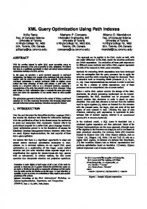
Note that while there are n rows in T = {r1 , r2 , . . . rn }, it is not necessarily true that the maximum row number M is the same as n, since a method is commonly used to associate a fixed number of rows p with each disk page for fast lookup. Thus for a given row r with row number j, the table page number accessed to retrieve row r is j/p and the page slot is (in C terms) j%p. This means that rows will be assigned row numbers in disk clustered sequence, a valuable property. Since the rows might have variable size and we may not always be able to accommodate an equal number of rows on each disk page, the value p must be a chosen as a maximum, so some integers in Z[M] might be wasted. They will correspond to non-existent slots on pages that cannot accommodate the full set of p rows. (And we may find that m-1(j) for some row numbers j in Z[M] is undefined.) A "Bitmap" B is defined on T as a sequence of M bits. If a Bitmap B is meant to list rows in T with a given property P, then for each row r with row number j that has the property P, we set bit j in B to one; all other bits are set to zero. A Bitmap index for a column C with values v1, v2, . . ., vk, is a B-tree with entries having these keyvalues and associated data portions that contain Bitmaps for the properties C = v1, . . ., C = vk. Thus Bitmaps in this index are just a new way to specify lists of RIDs for specific column values. See Figure 2.1 for an Example. Note that a series of successive Bitmap Fragments make up the entry for "department = 'sports'".

B-tree Root Node for department index 'clothes''china'... 'sports' ... 'tools'

' spor t s 101101 . . . ' spor t s 01011 . . ' ' . Figure 2.1. Example of a Bitmap Index on department, a column of the SALES table We say that Bitmaps are dense if the proportion of one-bits in the Bitmap is large. A Bitmap index for a column with 32 values will have Bitmaps with average density of 1/32. In this case the disk space to hold a Bitmap column index will be comparable to the disk space needed for a RID-list index (which requires about 32 bits for each RID present). While the uncompressed Bitmap index size is proportional to the number of column values, a RID-list index is about the same size for any number of values (as long as we can continue to amortize the keysize with a long block of RIDs). For a column index with a very small number of values, the Bitmaps will have high densities (such as 50% for predicates such as GENDER = 'M' or GENDER = 'F'), and the disk savings is enormous. On the other hand, when average Bitmap density for a Bitmap index becomes too low, methods exist for compressing a Bitmap. The simplest of these is to translate the Bitmap back to a RID list, and we will assume this in what follows. 2.1.2 Bitmap Index Performance

1B+-trees

are commonly referred to simply as B-trees in database documentation, and we will follow this convention.

An important consideration for database query performance is the fact that Boolean operations, such as AND, OR, and NOT are

-2-

extremely fast for Bitmaps. Given Bitmaps B1 and B2, we can calculate a new Bitmap B3, B3 = B1 AND B2, by treating all bitmaps as arrays of long ints and looping through them, using the & operation of C: for (i = 0; i < len(B1); i++) /* Note: len(B1)=len(B2)=len(B3) B3[i] = B1[i] & B2[i]; /* B3 = B1 AND B2

*/ */

We would not normally expect the entire Bitmap to be memory resident, but would perform a loop to operate on Bitmaps by reading them in from disk in long Fragments. We ignore this loop here. Using a similar approach, we can calculate B3 = B1 OR B2. But calculating B3 = NOT(B1) requires an extra step. Since some bit positions can correspond to non-existent rows, we postulate an Existence Bitmap (designated EBM) which has exactly those 1 bits corresponding to existing rows. Now when we perform a NOT on a Bitmap B, we loop through a long int array performing the ~ operation of C, then AND the result with the corresponding long int from EBM. for (i = 0; i < len(B1); i++) B3[i] = ~B1[i] & EBM[i]; /* B3 = NOT(B1)for rows that exist

*/

Typical Select statements may have a number of predicates in their Where Clause that must be combined in a Boolean manner. The resulting set of rows, which is then retrieved or aggregated in the Select target-list, is called a Foundset in what follows. Sometimes, the rows filtered by the Where Clause must be further grouped, due to a group-by clause, and we refer to the set of rows restricted to a single group as a Groupset. Finally, we show how the COUNT function for a Bitmap of a Foundset can be efficiently performed. First, a short int array shcount[ ] is declared, with entries initialized to contain the number of bits in the entry subscript. Given this array, we can loop through a Bitmap as an array of short int values, to get the count of the total Bitmap as shown in Algorithm 2.1. Clearly the shcount[ ] array is used to provide parallelism in calculating the COUNT on many bits at once. Algorithm 2.1. Performing COUNT with a Bitmap /* Assume B1[ ] is a short int array overlaying a Foundset Bitmap count = 0; for (i = 0; i < SHNUM; i++) count += shcount[B1[i]]; /* add count of bits for next short int u

*/

*/

Loops for Bitmap AND, OR, NOT, or COUNT are extremely fast compared to loop operations on RID lists, where several operations are required for each RID, so long as the Bitmaps involved have reasonably high density (down to about 1%). Example 2.1. In the Set Query benchmark of [O'NEI91], the results from one of the SQL statements in Query Suite Q5 gives a good illustration of Bitmap performance. For a table named BENCH of 1,000,000 rows, two columns named K10 and K25 have cardinalities 10 and 25, respectively, with all rows in the table equally likely to take on any valid value for either column. Thus the Bitmap densities for indexes on this column are 10% and 4% respectively. One SQL statement from the Q5 Suite is:

[2.1] SELECT K10, K25, COUNT(*) FROM BENCH GROUP BY K10, K25; A 1995 benchmark on a 66 MHz Power PC of the Praxis Omni Warehouse, a C language version of MODEL 204, demonstrated an elapsed time of 19.25 seconds to perform this query. The query plan was to read Bitmaps from the indexes for all values of K10 and K25, perform a double loop through all 250 pairs of values, AND all pairs of Bitmaps, and COUNT the results. The 250 ANDs and 250 COUNTs of 1,000,000 bit Bitmaps required only 19.25 seconds on a relatively weak processor. By comparison, MVS DB2 Version 2.3, running on an IBM 9221/170 used an algorithm that extracted and wrote out all pairs of (K10, K25) values from the rows, sorted by value pair, and counted the result in groups, taking 248 seconds of elapsed time and 223 seconds of CPU. (See [O'NEI96] for more details.) u 2.1.3 Segmentation To optimize Bitmap index access, Bitmaps can be broken into Fragments of equal sizes to fit on single fixed-size disk pages. Corresponding to these Fragments, the rows of a table are partitioned into Segments, with an equal number of row slots for each segment. In MODEL 204 (see [M204, O'NEI87]), a Bitmap Fragment fits on a 6 KByte page, and contains about 48K bits, so the table is broken into segments of about 48K rows each. This segmentation has two important implications. The first implication involves RID-lists. When Bitmaps are sufficiently sparse that they need to be converted to RID-lists, the RID-list for a segment is guaranteed to fit on a disk page (1/32 of 48K is about 1.5K; MODEL 204 actually allows sparser Bitmaps than 1/32, so several RID lists might fit on a single disk page). Furthermore, RIDs need only be two bytes in length, because they only specify the row position within the segment (the 48K rows of a segment can be counted in a short int). At the beginning of each RID-list, the segment number will specify the higher order bits of a longer RID (4 byte or more), but the segment-relative RIDs only use two bytes each. This is an important form of prefix RID compression, which greatly speeds up index range search. The second implication of segmentation involves combining predicates. The B-tree index entry for a particular value in MODEL 204 is made up of a number of pointers by segment to Bitmap or RID-list Fragments, but there are no pointers for segments that have no representative rows. In the case of a clustered index, for example, each particular index value entry will have pointers to only a small set of segments. Now if several predicates involving different column indexes are ANDed, the evaluation takes place segment-by-segment. If one of the predicate indexes has no pointer to a Bitmap Fragment for a segment, then the segment Fragments for the other indexes can be ignored as well. Queries like this can turn out to be very common in a workload, and the I/O saved by ignoring I/O for these index Fragments can significantly improve performance. In some sense, Bitmap representations and RID-list representations are interchangeable: both provide a way to list all rows with a given index value or range of values. It is simply the case that, when the Bitmap representations involved are relatively dense, Bitmaps are much more efficient than RID-lists, both in storage use and efficiency of Boolean operations. Indeed a Bitmap index can contain RID-lists for some entry values or even for some Segments within a value entry, whenever the number of rows with a given keyvalue would be too sparse in

-3-

the segment for a Bitmap to be efficiently used. In what follows, we will assume that a Bitmapped index combines Bitmap and RID-list representations where appropriate, and continue to refer to the hybrid form as a Value-List Index. When we refer to the Bitmap for a given value v in the index, this should be understood to be a generic name: it may be a Bitmap or it may be a RID-list, or a segment-by-segment combination of the two forms. 2.2 Projection Indexes Assume that C is a column of a table T; then the Projection index on C consists of a stored sequence of column values from C, in order by the row number in T from which the values are extracted. (Holes might exist for unused row numbers.) If the column C is 4 bytes in length, then we can fit 1000 values from C on each 4 KByte disk page (assuming no holes), and continue to do this for successive column values, until we have constructed the Projection index. Now for a given row number n = m(r) in the table, we can access the proper disk page, p, and slot, s, to retrieve the appropriate C value with a simple calculation: p = n/1000 and s = n%1000. Furthermore, given a C value in a given position of the Projection index, we can calculate the row number easily: n = 1000*p + s. If the column values for C are variable length instead of fixed length, there are two alternatives. We can set a maximum size and place a fixed number of column value on each page, as before, or we can use a B-tree structure to access the column value C by a lookup of the row number n. The case of variable-length values is obviously somewhat less efficient than fixed-length, and we will assume fixed-length C values in what follows. The Projection index turns out to be quite efficient in certain cases where column values must be retrieved for all rows of a Foundset. For example, if the density of the Foundset is 1/50 (no clustering, so the density is uniform across all table segments), and the column values are 4 bytes in length, as above, then 1000 values will fit on a 4 KByte page, and we expect to pick up 20 values per Projection index page. In contrast, if the rows of the table were retrieved, then assuming 200-byte rows only 20 rows will fit on a 4 KByte page, and we expect to pick up only 1 row per page. Thus reading the values from a Projection index requires only 1/20 the number of disk page access as reading the values from the rows. The Sybase IQ product is the first one to have utilized the Projection index heavily, under the name of "Fast Projection Index" [EDEL95, FREN95]. The definition of a Projection index is reminiscent of vertically partitioning the columns of a table. Vertical partitioning is a good strategy for workloads where small numbers of columns are retrieved by most Select statements, but it is a bad idea when most queries retrieve many most of the columns. Vertical partitioning is actually forbidden by the TPC-D benchmark, presumably on the theory that the queries chosen have not been sufficiently tuned to penalize this strategy. But Projection indexes are not the same as vertical partitioning. We assume that rows of the table are still stored in contiguous form (the TPC-D requirement) and the Projection indexes are auxiliary aids to retrieval efficiency. Of course this means that column values will be duplicated in the index, but in fact all traditional indexes duplicate column values in this same sense. 2.3.

Bit-Sliced Indexes

A Bit-Sliced index stores a set of "Bitmap slices" which are "orthogonal" to the data held in a Projection index. As we will see,

they provide an efficient means to calculate aggregates of Foundsets. We begin our definition of Bit-Sliced indexes with an example. Example 2.2. Consider a table named SALES which contains rows for all sales that have been made during the past month by individual stores belonging to some large chain. The SALES table has a column named dollar_sales, which represents for each row the dollar amount received for the sale. Now interpret the dollar_sales column as an integer number of pennies, represented as a binary number with N+1 bits. We define a function D(n, i), i = 0, . . . , N, for row number n in SALES, to have value 0, except for rows with a non-null value for dollar_sales, where the value of D(n, i) is defined as follows: D(n, 0) = 1 if the 1 bit for dollar_sales in row number n is on D(n, 1) = 1 if the 2 bit for dollar_sales in row number n is on . . . D(n, i) = 1 if the 2i bit for dollar_sales in row number n is on Now for each value i, i = 0 to N, such that D(n, i) > 0 for some row in SALES, we define a Bitmap Bi on the SALES table so that bit n of Bitmap Bi is set to D(n, I). Note that by requiring that D(n, i) > 0 for some row in SALES, we have guaranteed that we do not have to represent any Bitmap of all zeros. For a real table such as SALES, the appropriate set of Bitmaps with nonzero bits can easily be determined at Create Index time. u The definitions of Example 2.1 generalize to any column C in a table T, where the column C is interpreted as a sequence of bits, from least significant (i = 0) to most significant (i = N). Definition 2.1: Bit-Sliced Index. The Bit-Sliced index on the C column of table T is the set of all Bitmaps Bi as defined analogously for dollar_sales in Example 2.2. Since a null value in the C column will not have any bits set to 1, it is clear that only rows with non-null values appear as 1-bits in any of these Bitmaps. Each individual Bitmap Bi is called a Bit-Slice of the column. We also define the Bit-Sliced index to have a Bitmap B nn representing the set of rows with non-null values in column C, and a Bitmap Bn representing the set of rows with null values. Clearly Bn can be derived from Bnn and the Existence Bitmap EBM, but we want to save this effort in algorithms below. In fact, the Bitmaps Bnn and Bn are so useful that we assume from now on that Bnn exists for Value-List Bitmap indexes (clearly Bn already exists, since null is a particular value). u In the algorithms that follow, we will normally be assuming that the column C is numeric, either an integer or a floating point value. In using Bit-Sliced indexes, it is necessary that different values have matching decimal points in their binary representations. Depending on the variation in size of the floating point numbers, this could lead to an exceptionally large number of slices when values differ by many orders of magnitude. Such an eventuality is unlikely in business applications, however. A user-defined method to bit-slice aggregate quantities was used by some MODEL 204 customers and is defined on page 48 of [O'NEI87]. Sybase IQ currently provides a fully realized BitSliced index, which is known to the query optimizer and transparent to SQL users. Usually, a Bit-Sliced index for a quantity of the kind in Example 2.2 will involve a relatively small number of Bitmaps (less than the maximum significance), although there is no real limit imposed by the definition. Note that 20

-4-

Bitmaps, 0 . . .19, for the dollar_sales column will represent quantities up to 220 - 1 pennies, or $10,485.75, a large sale by most standards. If we assume normal sales range up to $100.00, it is very likely that nearly all values under $100.00 will occur for some row in a large SALES table. Thus, a Value-List index would have nearly 10,000 different values, and row-sets with these values in a Value-List index would almost certainly be represented by RID-lists rather than Bitmaps. The efficiency of performing Boolean Bitmap operations would be lost with a Value-List index, but not with a Bit-Sliced index, where all values are represented with about 20 Bitmaps. It is important to realize that these index types are all basically equivalent. Theorem 2.1. For a given column C on a table T, the information in a Bit-sliced index, Value-List index, or Projection index can each be derived from either of the others. Proof. With all three types of indexes, we are able to determine the values of columns C for all rows in T, and this information is sufficient to create any other index. u Although the three index types contain the same information, they provide different performance advantages for different operations. In the next few sections of the paper we explore this. 3. Comparing Index types for Aggregate Evaluation In this section we give algorithms showing how Value-List indexes, Projection indexes, and Bit-Sliced indexes can be used to speed up the evaluation of aggregate functions in SQL queries. We begin with an analysis evaluating SUM on a single column. Other aggregate functions are considered later.

The time to perform such a sequence of I/Os, assuming one disk arm retrieves 100 disk pages per second in relatively close sequence on disk, is 16,484 seconds, or more than 4 hours of disk arm use. We estimate 25 instructions needed to retrieve the proper row and column value from each buffer resident page, and this occurs 2,000,000 times, but in fact the CPU utilization associated with reading the proper page into buffer is much more significant. Each disk page I/O is generally assumed to require several thousand instructions to perform (see, for example, [PH96], Section 6.7, where 10,000 instructions are assumed). Query Plan 2: Calculating SUM with a Projection index. We can use the Projection index to calculate the sum by accessing each dollar_sales value in the index corresponding to a row number in the Foundset; these row numbers will be provided in increasing order. We assume as in Example 2.2 that the dollar_sales Projection index will contain 1000 values per 4 KByte disk page. Thus the Projection index will require 100,000 disk pages, and we can expect all of these pages to be accessed in sequence when the values for the 2,000,000 row Foundset are retrieved. This implies we will have 100,000 disk page I/Os, with elapsed time 1000 seconds (roughly 17 minutes), given the same I/O assumptions as in Query Plan 1. In addition to the I/O, we will use perhaps 10 instructions to convert the Bitmap row number into a disk page offset, access the appropriate value, and add this to the SUM. Query Plan 3: Calculating SUM with a Value-List index. Assuming we have a Value-List index on dollar_sales, we can calculate SUM(dollar_sales) for our Foundset by ranging through all possible values in the index and determining the rows with each value, then determining how many rows with each value are in the Foundset, and finally multiplying that count by the value and adding to the SUM. In pseudo code, we have Algorithm 3.1 below.

3.1 Evaluating Single-Column Sum Aggregates Example 3.1. Assume that the SALES table of Example 2.2 has 100 million rows which are each 200 bytes in length, stored 20 to a 4 KByte disk page, and that the following Select statement has been submitted: [3.1] SELECT SUM(dollar_sales) FROM SALES WHERE condition; The condition in the Where clause that restricts rows of the SALES table will result in a Foundset of rows. We assume in what follows that the Foundset has already been determined, and is represented by a Bitmap Bf, it contains 2 million rows and the rows are not clustered in a range of disk pages, but are spread out evenly across the entire table. We vary these assumptions later. The most likely case is that determining the Foundset was easily accomplished by performing Boolean operations on a few indexes, so the resources used were relatively insignificant compared to the aggregate evaluation to follow. Query Plan 1: Direct access to rows to calculate SUM. Each disk page contains only 20 rows, so there must be a total of 5,000,000 disk pages occupied by the SALES table. Since 2,000,000 rows in the Foundset Bf represent only 1/50 of all rows in the SALES table, the number of disk pages that the Foundset occupies can be estimated (see [O'NEI96], Formula [7.6.4]) as: 5 ,000,000(1 - e-2,000,000/5,000,000) = 1,648,400 disk pages

Algorithm 3.1. Evaluating SUM(C) with a Value-List Index If (COUNT(Bf AND Bnn) == 0) /* no non-null values * / Return null; SUM = 0.00; For each non-null value v in the index for C { Designate the set of rows with the value v as Bv SUM += v * COUNT(Bf AND Bv); } Return SUM; u Our earlier analysis counted about 10,000 distinct values in this index, so the Value-List index evaluation of SUM(C) requires 10,000 Bitmap ANDs and 10,000 COUNTs. If we make the assumption that the Bitmap B f is held in memory (100,000,000 bits, or 12,500,000 bytes) while we loop through the values, and that the sets Bv for each value v are actually RIDlists, this will entail 3125 I/Os to read in Bf , 100,000 I/Os to read in the index RID-lists for all values (100,000,000 RIDs of 4 bytes each, assuming all pages are completely full), and a loop of several instructions to translate 100,000,000 RIDs to bit positions and test if they are on in Bf. Note that this algorithm gains an enormous advantage by assuming Bf is a Bitmap (rather than a RID-list), and that it can be held in memory, so that RIDs from the index can be looked up quickly. If Bf were held as a RID-list instead, the lookup would be a good deal less efficient, and would probably entail a sort by RID value of values from the index, followed by a merge-inter-

-5-

sect with the RID-list Bf. Even with the assumption that Bf is a Bitmap in memory, the loop through 100,000,000 RIDs is extremely CPU intensive, especially if the translation from RID to bit ordinal entails a complex lookup in a memory-resident tree to determine the extent containing the disk page of the RID and the corresponding RID number within the extent. With optimal assumptions, Plan 3 seems to require 103,125 I/Os and a loop of length 100,000,000, with a loop body of perhaps 10 instructions. Even so, Query Plan 3 is probably superior to Query Plan 1, which requires I/O for 1,340,640 disk pages. Query Plan 4: Calculating SUM with a Bit-Sliced index. Assuming we have a Bit-Sliced index on dollar_sales as defined in Example 2.2, we can calculate SUM(dollar_sales) with the pseudo code of Algorithm 3.2. Algorithm 3.2. Evaluating SUM(C) with a Bit-Sliced Index / * We are given a Bit-Sliced index for C, containing bitmaps Bi, i = 0 to N (N = 19), Bn and Bnn, as in Example 2.2 and Definition 2.1. */ If (COUNT(Bf AND Bnn) == 0) Return null; SUM = 0.00 For i = 0 to N SUM += 2i * COUNT(Bi AND Bf); Return SUM; u With Algorithm 3.2, we can calculate a SUM by performing 21 ANDs and 21 COUNTs of 100,000,000 bit Bitmaps. Each Bitmap is 12.5 MBytes in length, requiring 3125 I/Os, but we assume that Bf can remain in memory after the first time it is read. Therefore, we need to read a total of 22 Bitmaps from disk, using 22*3125 = 68,750 I/Os, a bit over half the number needed in Query Plan 2. For CPU, we need to AND 21 pairs of Bitmaps, which is done by looping through the Bitmaps in long int chunks, a total number of loop passes on a 32-bit machine equal to: 21*(100,000,000/32) = 65,625,000. Then we need to perform 21 COUNTs, looping through Bitmaps in half-word chunks, with 131,250,000 passes. However, all these 196,875,000 passes to perform ANDs and COUNTs are single instruction loops, and thus presumably take a good deal less time than the 100,000,000 multi-instruction loops of Plan 2. 3.1.1 Comparing Algorithm Performance

submitted at a rate of once each 1,000 seconds, the most expensive plan, "Add from rows", will keep 13.41 disks busy at a cost of $8046 purchase. We calculate the number of CPU instructions needed for I/O for the various plans, with the varying assumptions in Table 3.2 of how many instructions are needed to perform an I/O. Adding the CPU cost for algorithmic loops to the I/O cost, we determine the total dollar cost ($Cost) to support the method. For example, for the "Add from Rows" plan, assuming one submission each 1000 seconds, if an I/O uses (2K, 5K, 10K) instructions, the CPU cost is ($32.78, $81.06, $161.52). The cost for disk access ($8046) clearly swamps the cost of CPU in this case, and in fact the relative cost of I/O compared to CPU holds for all methods. Table 3.2 shows that the Bit-sliced index is the most efficient for this problem, with the Projection index and Value-List index a close second and third. The Projection index is so much better than the fourth ranked plan of accessing the rows that one would prefer it even if thirteen different columns were to be summed, notwithstanding the savings to be achieved by summing all the different columns from the same memory-resident row. Method

Add from Rows Projection index Value-List index Bit-Sliced index

Table 3.2. Dollar costs of four plans for SUM 3.1.2 Varying Foundset Density and Clustering Changing the number of rows in the Foundset has little effect on the Value-List index or Bit-Sliced index algorithms, because the entire index must still be read in both cases. However, the algorithms Add from rows and using a Projection index entail work proportional to the number of rows in the foundset. We stop considering the plan to Add from rows in what follows. Suppose the Foundset contains kM (k million) rows, clustered on a fraction f of the disk space. Both the Projection and BitSliced index algorithms can take advantage of the clustering. The table below shows the comparison between the three index algorithms.

Table 3.1 compares the above four Query Plans to calculate SUM, in terms of I/O and factors contributing to CPU. Method Add from Rows Projection index Value-List index Bit-Sliced index

I/O 1,341K 100K 103K 69K

CPU contributions I/O + 2M*(25 ins) I/O + 2M *(10 ins) I/O + 100M *(10 ins) I/O + 197M *(1 ins)

Table 3.1. I/O and CPU factors for the four plans We can compare the four query plans in terms of dollar cost by converting I/O and CPU costs to dollar amounts, as in [GP87]. In 1997, a 2 GB hard disk with a 10 ms access time costs roughly $600. With the I/O rate we have been assuming, this is approximately $6.00 per I/O per second. A 200 MHz Pentium computer, which processes approximately 150 MIPS (million instructions per second), costs roughly $1800, or approximately $12.00 per MIPS. If we assume that each of the plans above is

$Cost for $Cost for $Cost for 2K ins 5K ins 10K ins per I/O per I/O per I/O $8079 $8127 $8207 $603 $606 $612 $632 $636 $642 $418 $421 $425

Method Projection index Value-List index Bit-Sliced index

I/O f . 100K 103K f . 69K

CPU contributions I/O + kM . (10 ins) I/O + 100M . (10 ins) I/O + f .197M . (1 ins)

Table 3.3. Costs of four plans, I/O and CPU factors, with kM rows and clustering fraction f Clearly there is a relationship between k and f in Table 3.3, since for k = 100, 100M rows sit on a fraction f = 1.0 of the table, we must have k ≤ f.100. Also, if f becomes very small compared to k/100, we will no longer pick up every page in the Projection or Bit-Sliced index. In what follows, we assume that f is sufficiently large that the I/O approximations in Table 3.3 are valid. The dollar cost of I/O continues to dominate total dollar cost of the plans when each plan is submitted once every 1000 seconds. For the Projection index, the I/O cost is f.$600. The CPU cost,

-6-

assuming that I/O requires 10K instructions is: ((f.100 .10,000+k .1000 .10)/1,000,000).$12. Since k ≤ f.100, the formula f.100.10,000 + k.1000.10 ≤ f.100.10,000 + f.100.1000.10 = f.2,000,000. Thus, the total CPU cost is bounded above by f.$24, which is still cheap compared to an I/O cost of f.$600. Yet this is the highest cost we assume for CPU due to I/O, which is the dominant CPU term. In Table 3.4, we give the maximum dollar cost for each index approach. Method Projection index Value-List index Bit-Sliced index

$Cost for 10K ins per I/O f.$624 $642 f.$425

Table 3.4. Costs of the four plans in dollars, with kM rows and clustering fraction f The clustered case clearly affects the plans by making the Projection and Bit-Sliced indexes more efficient compared to the Value-List index. 3.2 Evaluating Other Column Aggregate Functions We consider aggregate functions of the form in [3.2], where AGG is an aggregate function, such as COUNT, MAX, MIN, etc. [3.2] SELECT AGG(C) FROM T

WHERE condition;

Table 3.5 lists a group of aggregate functions and the index types to evaluate these functions. We enter the value "Best" in a cell if the given index type is the most efficient one to have for this aggregation, "Slow" if the index type works but not very efficiently, etc. Note that Table 3.5 demonstrates how different index types are optimal for different aggregate situations. Aggregate

Value-List Index COUNT Not needed SUM Not bad AVG ( SUM/COUNT) Not bad MAX and MIN Best MEDIAN, N-TILE Usually Best Column-Product Very Slow

Projection Index Not needed Good Good Slow Not Useful Best

Bit-Sliced Index Not needed Best Best Slow Sometimes Best 2 Very Slow

Table 3.5. Tabulation of Performance by Index Type for Evaluating Aggregate Functions The COUNT and SUM aggregates have already been covered. COUNT requires no index, and AVG can be evaluated as SUM/COUNT, with performance determined by SUM. The MAX and MIN aggregate functions are best evaluated with a Value-List index. To determine MAX for a Foundset Bf, one loops from the largest value in the Value-List index down to the smallest, until finding a row in Bf. To find MAX and MIN using a Projection index, one must loop through all values stored. The algorithm to evaluate MAX or MIN using a Bit-Sliced index is given in our extended paper, [O'NQUA], together with other algorithms not detailed in this Section. 2Best

only if there is a clustering of rows in B in a local region, a fraction f of the pages, f ≤ 0.755.

To calculate MEDIAN(C) with C a keyvalue in a Value-List index, one loops through the non-null values of C in decreasing (or increasing) order, keeping a count of rows encountered, until for the first time with some value v the number of rows encountered so far is greater than COUNT(Bf AND Bnn )/2. Then v is the MEDIAN. Projection indexes are not useful for evaluating MEDIAN, unless the number of rows in the Foundset is very small, since all values have to be extracted and sorted. Surprisingly, a Bit-Sliced index can also be used to determine the MEDIAN, in about the same amount of time as it takes to determine SUM (see [O'NQUA]). The N-TILE aggregate function finds values v1 , v2 , . . ., vN-1 , which partition the rows in Bf into N sets of (approximately) equal size based on the interval in which their C value falls: C = c1, C = c1, C >= c1, C > c1, C between c1 and c2}, where c1 and c2 are constant values. We will demonstrate below how to further restrict the Foundset Bf, creating a new Foundset BF, so that the compound predicate "C-range AND " holds for exactly those rows contained in B F. We do this with varying assumptions regarding index types on the column C. Evaluating the Range using a Projection Index. If there is a Projection index on C, we can create BF by accessing each C value in the index corresponding to a row number in Bf and testing whether it lies within the specified range. Evaluating the Range using a Value-List Index. With a Value-List index, evaluation the C-range restriction of [4.1] uses an algorithm common in most database products, looping through the index entries for the range of values. We vary slightly by accumulating a Bitmap Br as an OR of all row sets in the index for values that lie in the specified range, then AND this result with Bf to get BF. See Algorithm 4.1. Note that for Algorithm 4.1 to be efficiently performed, we must find some way to guarantee that the Bitmap Br remains in memory at all times as we loop through the values v in the range. This requires some forethought in the Query Optimizer if the table T

-7-

being queried is large: 100 million rows will mean that a Bitmap Br of 12.5 MBytes must be kept resident.

to test each value and, if the row passes the range test, to turn on the appropriate bit in a Foundset.

Algorithm 4.1. Range Predicate with a Value-List Index Br = the empty set For each entry v in the index for C that satisfies the range specified Designate the set of rows with the value v as Bv Br = Br OR Bv BF = Bf AND Br u

As we have just seen, it is possible to determine the Foundset of rows in a range using Bit-Sliced indexes. We can calculate the range predicate c2 >= C >= c1 using a Bit-Sliced index by calculating BGE for c1 and BLE for c2, then ANDing the two. Once again the calculation is generally comparable in cost to calculating a SUM aggregate, as seen in Fig. 3.2.

Evaluating the Range using a Bit-Sliced Index. Rather surprisingly, it is possible to evaluate range predicates efficiently using a Bit-Sliced index. Given a Foundset Bf, we demonstrate in Algorithm 4.2 how to evaluate the set of rows BGT such that C > c1, BGE such that C >= c1, BEQ such that C = c1, BLE such that C = c1, we don't need steps that evaluate BLE or BLT. Algorithm 4.2. Range Predicate with a Bit-Sliced Index BGT = BLT = the empty set; BEQ = Bnn For each Bit-Slice Bi for C in decreasing significance If bit i is on in constant c1 BLT = BLT OR (BEQ AND NOT(Bi)) BEQ = BEQ AND Bi else BGT = BGT OR (BEQ AND Bi) BEQ = BEQ AND NOT(Bi) BEQ = BEQ AND Bf; BGT = BGT AND Bf; BLT = BLT AND Bf BLE = BLT OR BEQ; BGE = BGT OR BEQ u Proof that BEQ BGT and BGE are properly evaluated. The method to evaluate BEQ clearly determines all rows with C = c1, since it requires that all 1-bits on in c1 be on and all 0-bits 0 in c1 be off for all rows in BEQ. Next, note that BGT is the OR of a set of Bitmaps with certain conditions, which we now describe. Assume that the bit representation of c1 is bN b N-1 . . .b1 b 0 , and that the bit representation of C for some row r in the database is rNrN-1. . .r1r0. For each bit position i from 0 to N with bit bi off in c1, a row r will be in BGT if bit ri is on and bits rNrN-1. . .r1ri+1 are all equal to bits bN b N-1 . . .bi+1 . It is clear that C > c1 for any such row r in BGT . Furthermore for any value of C > c1, there must be some bit position i such that the i-th bit position in c1 is off, the i-th bit position of C is on, and all more-significant bits in the two values are identical. Therefore, Algorithm 4.2 properly evaluates BGT. u

With a Value-List index, algorithmic effort is proportional to the width of the range, and for a wide range, it is comparable to the effort needed to perform SUM for a large Foundset. Thus for wide ranges the Projection and Bit-Sliced indexes have a performance advantage. For short ranges the work to perform the Projection and Bit-Sliced algorithms remain nearly the same (assuming the range variable is not a clustering value), while the work to perform the Value-List algorithm is proportional to the number of rows found in the range. Eventually as the width of the range decreases the Value-List algorithm is the better choice. These considerations are summarized in Table 4.1. Range Evaluation Value-List Index Narrow Range Best Wide Range Not bad

Projection Index Good Good

Bit-Sliced Index Good Best

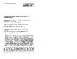
Table 4.1. Range Evaluation Performance by Index Type 4.2 Range Predicate with a Non-Binary Bit-Sliced Index Sybase IQ was the first product to demonstrate in practice that the same Bit-Sliced index, called the "High NonGroup Index" [EDEL95], could be used both for evaluating range predicates (Algorithm 4.2) and performing Aggregates (Algorithm 3.2, et al). For many years, MODEL 204 has used a form of indexing to evaluate range predicates, known as "Numeric Range" [M204]. Numeric Range evaluation is similar to Bit-Sliced Algorithm 4.2, except that numeric quantities are expressed in a larger base (base 10). It turns out that the effort of performing a range retrieval can be reduced if we are willing to store a larger number of Bitmaps. In [O'NQUA] we show how Bit-Sliced Algorithm 4.2 can be generalized to base 8, where the Bit-Slices represent sets of rows with octal digit Oi ≥ c, c a non-zero octal digit. This is a generalization of Binary Bit-Slices, which represent sets of rows with binary digit Bi ≥ 1. 5. Evaluating OLAP-style Queries Figure 5.1 pictures a star-join schema with a central fact table, SALES, containing sales data, together with dimension tables known as TIME (when the sales are made), PRODUCT (product sold), and CUSTOMER (purchaser in the sale). Most OLAP products do not express their queries in SQL, but much of the work of typical OLAP queries could be represented in SQL [GBLP96] (although more than one query might be needed).

4.1 Comparing Algorithm Performance Now we compare performance of these algorithms to evaluate a range predicate, "C between c1 and c2". We assume that C values are not clustered on disk. The cost of evaluating a range predicate using a Projection index is similar to evaluating SUM using a Projection index, as seen in Fig. 3.2. We need the I/O to access each of the index pages with C values plus the CPU cost

[5.1] SELECT P.brand, T.week, C.city, SUM(S.dollar_sales) FROM SALES S, PRODUCT P, CUSTOMER C, TIME T WHERE S.day = T.day and S.cid = C.cid and S.pid = P.pid and P.brand = :brandvar and T.week >= :datevar and C.state in ('Maine', 'New Hampshire', 'Vermont', 'Massachusetts', 'Connecticut', 'Rhode Island') GROUP BY P.brand, T.week, C.city;

-8-

Query [5.1] retrieves total dollar sales that were made for a product brand during the past 4 weeks to customers in New England. P RO DUCT Dime ns ion

CUS TO ME R Dime ns ion cid gender city state zip hobby TI ME Dime ns io n

S ALE S Fa c t cid pid day dollar_sales dollar_cost unit_sales

pid SKU brand size weight package_type

day week month year holiday_flg weekday_flg Figure 5.1. Star Join Schema of SALES, CUSTOMER, PRODUCT, and TIME An important advantage of OLAP products is evaluating such queries quickly, even though the fact tables are usually very large. The OLAP approach precalculates results of some Grouped queries and stores them in what we have been calling summary tables. For example, we might create a summary table where sums of Sales.dollar_sales and sums of Sales.unit_sales are precalculated for all combination of values at the lowest level of granularity for the dimensions, e.g., for C.cid values, T.day values, and P.pid values. Within each dimension there are also hierarchies sitting above the lowest level of granularity. A week has 7 days and a year has 52 weeks, and so on. Similarly, a customer exists in a geographic hierarchy of city and state. When we precalculate a summary table at the lowest dimensional level, there might be many rows of detail data associated with a particular cid, day, and pid (a busy product reseller customer), or there might be none. A summary table, at the lowest level of granularity, will usually save a lot of work, compared to detailed data, for queries that group by attributes at higher levels of the dimensional hierarchy, such as city (of customers), week, and brand. We would typically create many summary tables, combining various levels of the dimensional hierarchies. The higher the dimensional levels, the fewer elements in the summary table, but there are a lot of possible combinations of hierarchies. Luckily, we don't need to create all possible summary tables in order to speed up the queries a great deal. For more details, see [STG95, HRU96]. By doing the aggregation work beforehand, summary tables provide quick response to queries, so long as all selection conditions are restrictions on dimensions that have been foreseen in advance. But, as we pointed out in Example 1.1, if some restrictions are non-dimensional, such as temperature, then summary tables sliced by dimensions will be useless. And since the size

of data in the summary tables grows as the product of the number of values in the independent dimensions (counting values of hierarchies within each dimension), it soon becomes impossible to provide dimensions for all possible restrictions. The goal of this section is to describe and analyze a variant indexing approach that is useful for evaluating OLAP-style queries quickly, even when the queries cannot make use of preaggregation. To begin, we need to explain Join indexes. 5.1 Join Indexes Definition 5.1. Join Index. A Join index is an index on one table for a quantity that involves a column value of a different table through a commonly encountered join u Join indexes can be used to avoid actual joins of tables, or to greatly reduce the volume of data that must be joined, by performing restrictions in advance. For example, the Star Join index — invented a number of years ago — concatenates ordinal encodings of column values from different dimension tables of a Star schema, and lists RIDs in the central fact table for each concatenated value. The Star Join index was the best approach known in its day, but there is a problem with it, comparable to the problem with summary tables. If there are numerous columns used for restrictions in each dimension table, then the number of Star Join indexes needed to be able to combine arbitrary column restrictions from each dimension table is a product of the number of columns in each dimension. Thus, there will be a "combinatorial explosion" of Join Indexes in terms of the number of independent columns. The Bitmap join index, defined in [O'NGG95], addresses this problem. In its simplest form, this is an index on a table T based on a single column of a table S, where S commonly joins with T in a specified way. For example, in the TPC-D benchmark database, the O_ORDERDATE column belongs to the ORDER table, but two TPC-D queries need to join ORDER with LINEITEM to restrict LINEITEM rows to a range of O_ORDERDATE. This can better be accomplished by creating an index for the value ORDERDATE on the LINEITEM table. This doesn't change the design of the LINEITEM table, since the index on ORDERDATE is for a virtual column through a join. The number of indexes of this kind increases linearly with the number of useful columns in all dimension tables. We depend on the speed of combining Bitmapped indexes to create adhoc combinations, and thus the explosion of Star Join indexes because of different combinations of dimension columns is not a problem. Another way of looking at this is that Bitmap join indexes are Recombinant, whereas Star join indexes are not. The variant indexes of the current paper lead to an important point, that Join indexes can be of any type: Projection, ValueList, or Bit-Sliced. To speed up Query [5.1], we use Join indexes on the SALES fact table for columns in the dimensions. If appropriate join indexes exist for all dimension table columns mentioned in the queries, then explicit joins with dimension tables may no longer be necessary at all. Using Value-List or BitSliced join indexes we can evaluate the selection conditions in the Where Clause to arrive at a Foundset on SALES, and using Projection join indexes we can then retrieve the dimensional values for the Query [5.1] target-list, without any join needed. 5.2 Calculating Groupset Aggregates We assume that in star-join queries like [5.1], an aggregation is performed on columns of the central fact table, F. There is a

-9-

Foundset of rows on the fact table, and the group-by columns in the Dimension tables D1, D2, . . . (they might be primary keys of the Dimension tables, in which case they will also exist as foreign keys on F). Once the Foundset has been computed from the Where Clause, the bits in the Foundset must be partitioned into groups, which we call Groupsets, again sets of rows from F. Any aggregate functions are then evaluated separately over these different Groupsets. In what follows, we describe how to compute Groupset aggregates using our different index types. Computing Groupsets Using Projection Indexes. We assume Projection indexes exist on F for each of the group-by columns (these are Join Indexes, since the group-by columns are on the Dimension tables), and also for all columns of F involved in aggregates. If the number of group cells is small enough so that all grouped aggregate values in the target list will fit into memory, then partitioning into groups and computing aggregate functions for each group can usually be done rather easily. For each row of the Foundset returned by the Where clause, classify the row into a group-by cell by reading the appropriate Projection indexes on F. Then read the values of the columns to be aggregated from Projection indexes on these columns, and aggregate the result into the proper cell of the memory-resident array. (This approach can be used directly for functions such a SUM(C); for functions such as AVG(C), it can be done by accumulating a "handle" of results, SUM(C) and COUNT(C), to calculate the final aggregate.) If the total set of cells in the group-by cannot be retained in a memory-resident array, then the values to be aggregated can be tagged with their group cell values, and then values with identical group cell values brought together using a disk sort (this is a common method used today, not terribly efficient). Computing Groups Using Value-List Indexes. The idea of using Value-List indexes to compute aggregate groups is not new. As mentioned in Example 2.1, Model 204 used them years ago. In this section we formally present this approach. Algorithm 5.1. Grouping by columns D1.A, D2.B using a Value-List Index For each entry v1 in the Value-List index for D1.A For each entry v2 in the Value-List index for D2.B B g = Bv1 AND Bv2 AND Bf Evaluate AGG(F.C) on Bg /* We would do this with a Projection index */ u

be few rows in each, and evaluating the Grouped AGG(F.C) in Algorithm 5.1 might require an I/O for each individual row. 5.3 Improved Grouping Efficiency Using Segmentation and Clustering In this section we show how segmentation and clustering can be used to accelerate a query with one or more group-by attributes, using a generalization of Algorithm 5.1. We assume that the rows of the table F are partitioned into Segments, as explained in Section 2.1. Query evaluation is performed on one Segment at a time, and the results from evaluating each Segment are combined at the end to form the final query result. Segmentation is most effective when the number of rows per Segment is the number of bits that will fit on a disk page. With this Segment size, we can read the bits in an index entry that correspond to a segment by performing a single disk I/O. As pointed out earlier, if a Segment s1 of the Foundset (or Groupset) is completely empty (i.e., all bits are 0), then ANDing s 1 with any other Segment s2 will also result in an empty Segment. As explained in [O'NEI87], the entry in the B-tree leaf level for a column C that references an all-zeros Bitmap Segment is simply missing, and a reasonable algorithm to AND Bitmaps will test this before accessing any Segment Bitmap pages. Thus neither s1 nor s2 will need be read from disk after an early phase of evaluation. This optimization becomes especially useful when rows are clustered on disk by nested dimensions used in grouping, as we will see. Consider a Star Join schema with a central fact table F and a set of three dimension tables, D1, D2, D3. We can easily generalize the analysis that follows to more than three dimensions. Each dimension Dm, 1 ≤ m ≤ 3, has a primary key, dm , with a domain of values having an order assigned by the DBA. We represent the number of values in the domain of dm by nm , and list the values of dm in increasing order, differentiated by superscript, as: dm 1, n dm2, . . ., dm m. For example, the primary key of the TIME dimension of Figure 5.1 would be days and have a natural temporal order. The DBA would probably choose the order of values in the PRODUCT dimension so that the most commonly used hierarchies, such as product_type or category, consist of contiguous sets of values in the dimensional order. See Figure 5.2. Category

Algorithm 5.1 presents an algorithm for computing aggregate groups that works for queries with two group-by columns (with Bitmap Join Value-List indexes on Dimension tables D1 and D2). The generalization of Algorithm 5.1 to the case of n groupby attributes is straightforward. Assume the Where clause condition already performed resulted in the Foundset Bf on the fact table F. The algorithm generates a set of Groupsets, Bg, one for each (D1.A, D2.B) group. The aggregate function AGG(F.C) is evaluated for each group using Bg in place of Bf. Algorithm 5.1 can be quite inefficient when there are a lot of Groupsets and rows of table F in each Groupset are randomly placed on disk. The aggregate function must be re-evaluated for each group and, when the Projection index for the column F.C is too large to be cached in memory, we must revisit disk pages for each Groupset. With many Groupsets, we would expect there to

Personal Hygiene

Product Type

Soap

Shampoo

Product

PROD1 PROD2 PROD3 PROD4 PROD5 PROD6 PROD7 PROD8

Figure 5.2. Order of Values in PRODUCT Dimensions In what follows, we will consider a workload of OLAP-type queries which have group-by clauses on some values in the dimension tables (not necessarily the primary key values). The fact table F contains foreign key columns that match the primary keys of the various dimensions. We will assume indexes on these foreign keys for table F and make no distinction between these and these and the primary keys of the Dimensions. We in-

-10-

tend to demonstrate how these indexes can be efficiently used to perform group-by queries using Algorithm 5.1. We wish to cluster the fact table F to improve performance of the most finely divided group-by possible (grouping by primary key values of the dimensions rather than by any hierarchy values above these). It will turn out that this clustering is also effective for arbitrary group-by queries on the dimensions. To evaluate the successive Groupsets by Algorithm 5.1, we consider performing the nested loop of Figure 5.3. For each key-value v1 in order from D1 For each key-value v2 in order from D2 For each key-value v3 in order from D3 End For v3 End For v2 End For v1 Figure 5.3. Nested Loop to Perform a Group-By In the loop of Figure 5.3, we assume the looping order for dimensions (D1, D2, D3) is determined by the DBA (this order has long-term significance; we give an example below). The loop on dimension values here produces conjoint cells (v1, v2, v3), of the group-by. Each cell may contain a large number of rows from table F or none. The set of rows in a particular cell is what we have been referring to as a Groupset. It is our intent to cluster the rows of the fact table F so that all the rows with foreign keys matching the dimension values in each cell (v1 , v2 , v3 ) are placed together on disk, and furthermore that the successive cells fall in the same order on disk as the nested loop above on (D1, D2, D3). Given this clustering, the Bitmaps for each Groupset will have 1-bits in a limited contiguous range. Furthermore, as the loop is performed to calculate a group-by, successive cells will have rows in Groupset Bitmaps that are contiguous one to another and increase in row number. Figure 5.4 gives a schematic representation of the Bitmaps for index values of three dimensions. D 1 = d11 1111111111111111100000000000000000000... = d12 0000000000000000011111111111111111000... . . . D 2 = d21 1111111000000000011111110000000000111... = d22 0000000111111100000000001111111000000... . . . D 3 = d31 1100000110000000011000000000000000110... = d32 0011000001100000000110000000000000001... . . . n = d3 3 0000011000001100000000110000000000001... Figure 5.4. Schematic Representation of Dimension Index Bitmaps for Clustered F The Groupset Bitmaps are calculated by ANDing the appropriate index Bitmaps for the given values. Note that as successive Groupset Bitmaps in loop order are generated from ANDing, the 1-bits in each Groupset move from left to right. In terms of Figure 5.4, the Groupset for the first cell (d1 1 , d2 1 , d3 1 ) calculated by a Bitmap AND of the three index Bitmaps D1 = d11, D2 = d21, and D3 = d31, is as follows. 1100000000000000000000000000000000000...

The Groupset for the next few cells will have Bitmaps: 0011000000000000000000000000000000000... 0000110000000000000000000000000000000... And so on, moving from left to right. To repeat: as the loop to perform the most finely divided groupby is performed, and Groupset Bitmaps are generated, successive blocks of 1-bits by row number will be created, and successive row values from the Projection index will be accessed to evaluate an aggregate. Because of Segmentation, no unnecessary I/Os are ever performed to AND the Bitmaps of the individual dimensions. Indeed, due to clustering, it is most likely that Groupset Bitmaps for successive cells will have 1-bits that move from left to right on each Segment Bitmap page of the Value index, and the column values to aggregate will move from left to right in each Projection index page, only occasionally jumping to the next page. This is tremendously efficient, since relevant pages from the Value-list dimension indexes and Projection indexes on the fact table need be read only once from left to right to perform the entire group-by. If we consider group-by queries where the Groupsets are less finely divided than in the primary key loop given, grouping instead by higher hierarchical levels in the dimensions, this approach should still work. We materialize the grouped Aggregates in memory, and aggregate in nested loop order by the primary keys of the dimensions as we examine rows in F. Now for each cell, (v1 , v2 , v3 ) in the loop of Figure 5.3, we determine the higher order hierarchy values of the group-by we are trying to compute. Corresponding to each dimension primary m key value of the current cell, vi = di , there is a value in the dir mension hierarchy we are grouping by hi ; thus, as we loop through the finely divided cells, we aggregate the results for m m m r r r (d1 1, d2 2, d3 3) into the aggregate cell for (h1 1, h2 2, h3 3). As long as we can hold all aggregates for the higher hierarchical levels in memory at once, we have lost none of the nested loop efficiency. This is why we attempted to order the lowest level dimension values by higher level aggregates, so the cells here can be materialized, aggregated, and stored on disk in a streamed fashion. In a similar manner, if we were to group by only a subset of dimensions, we would be able to treat all dimensions not named as the highest hierarchical level for that dimension, which we refer to as ALL, and continue to use this nested loop approach. 5.4 Groupset Indexes While Bitmap Segmentation permits us to use normal Value-List indexing, ANDing Bitmaps (or RID-lists) from individual indexes to find Groupsets, there is some inefficiency associated with calculating which Segments have no 1-bits for a particular Cell to save ANDing segment Bitmaps. In Figure 5.1, for example, the cell (d1 1 , d2 1 , d3 1 ) has only the leftmost 2 bits on, but the Value-List index Bitmaps for these values have many other segments with bits on, as we see in Figure 5.4, and Bitmaps for individual index values might have 1-bits that span many Segments. To reduce this overhead, we can create a Groupset index, whose keyvalues are a concatenation of the dimensional primary-key values. Since the Groupset Bitmaps in nested loop order are represented as successive blocks of 1-bits in row number, the

-11-

Groupset index value can be represented by a simple integer, which represents the starting position of the first 1-bit in the Groupset, and the ending position of that Bitmap can be determined as one less than the starting position for the following index entry. Some cells will have no representative rows, and this will be most efficiently represented in the Groupset index by the fact that there is no value representing a concatenation of the dimensional primary-key values. We believe that the Groupset index makes the calculation of a multi-dimensional group-by as efficient as possible when precalculating aggregates in summary tables isn't appropriate. 6. Conclusion The read-mostly environment of data warehousing has made it feasible to use more complex index structures to speed up the evaluation of queries. This paper has examined two new index structures: Bit-Sliced indexes and Projection indexes. Indexes like these were used previously in commercial systems, Sybase IQ and MODEL 204, but never examined in print. As a new contribution, we have shown how ad-hoc OLAPstyle queries involving aggregation and grouping can be efficiently evaluated using indexing and clustering, and we have introduced a new index type, Groupset indexes, that are especially well-suited for evaluating this type of query.

[O'NEI91] Patrick O'Neil. The Set Query Benchmark. The Benchmark Handbook for Database and Transaction Processing Systems, Jim Gray (Ed.), Morgan Kaufmann, 2nd Ed. 1993, pp. 359-395. [O'NEI96] Patrick O'Neil. Database: Principles, Programming, and Performance. Morgan Kaufmann, 3rd printing, 1996. [O'NGG95] Patrick O'Neil and Goetz Graefe. Multi-Table Joins Through Bitmapped Join Indices. SIGMOD Record, September, 1995, pp. 8-11, [O'NQUA] Patrick O'Neil and Dallan Quass. Improved Query Performance with Variant Indexes. Extended paper, available on http:/www.cs.umb.edu/~poneil/varindexx.ps [PH96] D. A. Patterson and J. L. Hennessy. Computer Architecture, A Quantitative Approach. Morgan Kaufmann, 1996. [STG95] Stanford Technology Group, Inc., An INFORMIX Co.. Designing the Data Warehouse on Relational Databases. Informix White Paper, 1995, http://www.informix.com. [TPC] TPC Home Page. Descriptions and results of TPC benchmarks, including the TPC-C and TPC-D benchmarks. http://www.tpc.org.

References [COMER79] Comer, D. The Ubiquitous B-tree. Comput. Surv. 11 (1979), pp. 121-137. [EDEL95] Herb Edelstein. Faster Data Warehouses. Information Week, Dec. 4, 1995, pp. 77-88. Give title and author on http://www.techweb.com/search/advsearch.html. [FREN95] Clark D. French. "One Size Fits All" Database Architectures Do Not Work for DSS. Proceedings of the 1995 ACM SIGMOD Conference, pp. 449-450. [GBLP96] Jim Gray, Adam Bosworth, Andrew Layman, and Hamid Pirahesh. Data Cube: A Relational Operator Generalizing Group-By, Cross-Tab, and Sub-Totals. Proc. 12th Int. Conf. on Data Eng., pp. 152-159, 1996. [GP87] Jim Gray and Franco Putzolu. The Five Minute Rule for Trading Memory for Disk Accesses and The 10 Byte Rule for Trading Memory for CPU Time. Proc. 1987 ACM SIGMOD, pp. 395-398. [HRU96] Venky Harinarayan, Anand Rajaraman, and Jeffrey D. Ullman. Implementing Data Cubes Efficiently. Proc. 1996 ACM SIGMOD, pp. 205-216. [KIMB96] Ralph Kimball. The Data Warehouse Toolkit. John Wiley & Sons, 1996. [M204] MODEL 204 File Manager's Guide, Version 2, Release 1.0, April 1989, Computer Corporation of America. [O'NEI87] Patrick O'Neil. Model 204 Architecture and Performance. Springer-Verlag Lecture Notes in Computer Science 359, 2nd Int. Workshop on High Performance Transactions Systems (HPTS), Asilomar, CA, 1987, pp. 40-59.

-12-