Improved Rules for the Resource Allocation Design - DSS - TUM

Improved Rules for the Resource Allocation Design Pasha Shabalin, Bernd Laqua and Alexander Pikovsky Internet-based Information Systems, Dept. of Informatics, TU M¨unchen, Germany∗ {shabalin, laqua, pikovsky}@in.tum.de

Abstract Iterative Combinatorial Auctions (ICA) have been getting increasing attention both from researchers and in practice as they can increase efficiency of complex markets with substitute or complement valuations. This paper suggests several improvements for such auctions. We analyze the impact of these rules along several performance measurements using numerical simulations under various value models. Based on these simulations we select successful rules and consider their possible combinations.

1

Introduction

In Combinatorial Auctions several items are sold simultaneously and bidders can submit bundle bids. Such bids declare a single ask price for a subset of items, and the bidder can either win the complete subset or nothing, but not just a part of it. This solves the exposure problem of receiving just some of complement items, and consequently suffering economical losses. Thus Combinatorial Auctions allow bidders to better communicate their valuations, and to achieve better market efficiency compared to, for example, simultaneous multi-item auctions [5]. With growing adoption of electronic commerce, Combinatorial Auctions find broad practical applications. Examples include industrial procurement, selling of communication spectrum licenses, service contracts for bus routes and airport slots. Combinatorial Auctions have been adopted, among others, by Procter&Gamble, Wal-Mart, Bridgestone, Ford, Compaq, Staples [6]. In a Combinatorial Auction with m items 2m bundles can be built and used by bidders. This combinatorial explosion results in two hard problems. The auctioneer must solve the Winner Determination Problem (WDP), also called Combinatorial Allocation Problem (CAP). It lies in selecting the most valuable combination of bids under restriction that each item can be sold only once. Bidders have ∗ Financial support from the Deutsche Forschungsgemeinschaft (DFG) (BI 1057/1-1) is gratefully acknowledged.

to solve the Preference Elicitation Problem (PEP) - to find most valuable bundles, which in the general case requires evaluation of all 2m bundles. The CAP has been extensively studied in literature. It can be interpreted as a weighted set packing problem (SPP) - an NP-complete problem [10]. To solve CAP, along with traditional methods of Operation Research, there exist several CA-specific heuristics [17, 8]. For some restricted cases the CAP can be solved in polynomial time [4, 16]. There is much less research addressing the PEP. In practice it combines with the bidder’s strategy, and therefore can be solved analytically only under strict assumption regarding bidders’ behavior, usually myopic best response bidding [14]. An established method of mitigating the PEP is conducting of the auction in several rounds - Iterative Combinatorial Auctions (ICA). In each round bidders receive prices and optionally further information about the auction state (e.g. provisional allocation). This information shall help bidders to reduce bundle search space. In this work we consider ICAs with linear prices, where ask price of a bundle is defined as a sum of individual item ask prices. There are few theoretical results on linear prices in ICA, and therefore we build our research on numerical simulations. We base our tests on the RAD ICA design [9] as it uses intuitive pseudo-dual pricing model, and suggest several possible improvements on it. We analyze the impact of each improvement separately, and define those which improve the auction results. Further we measure the impact of the selected set of improvements on the auction outcome. The rest of this work has the following structure. Section 2 presents theoretical background on ICA. Section 3 describes suggestions for improved ICA rules. Section 4 describes simulation framework and parameters. Section 5 analyzes obtained results and practical applicability of the new ICA rules. Finally Section 6 concludes the work and discusses further research directions.

2

ICA with Linear Prices

We take a closer look at the CAP. Let K = {1, . . . , m} denote the set of items in the auction, indexed by k, and I = {1, . . . , n} denote the set of participating bidders, indexed by i. Let vi (S) ≥ 0 indicate the private valuation of bidder i for a bundle S ⊆ K. For an allocation X, the binary decision variable xi (S) indicates if bidder i’s bid on bundle S belongs to this allocation, i.e. X = {xi (S)}. The CAP has the following straightforward formulation. The linear program maximizes the sum of winning bids under the restriction that each item can be sold at most once. max

P P

xi (S) S⊆K i∈I

s.t. P P

xi (S)vi (S)

xi (S) ≤ 1

∀k ∈ K

(CAP)

S:k∈S i∈I

∈

xi (S)

{0, 1}

∀i, S

The central problem in the auction design is that the CAP requires values vi (S) for 2m bundles and for each bidder to be known to the auctioneer. Technically it is impractical for both time and space reasons. Furthermore there is a strategic problem: bidders are reluctant to submit their true valuations as they want to get goods cheaper, and prefer not to reveal their true preferences. ICA addresses this problem by using bid prices bti (S) in round t instead of valuations to calculate the provisional allocation. In each round t, the set of active bids B t is considered. Let B tk denote the set of all round t bids, containing item k. xb are binary decision variables, indicating winning state of corresponding bids: P

max

b∈B t

s.t. P

bti (S)xb

xb

≤ 1

∀k ∈ K

xb

∈

∀b

(CAP ICA)

b∈B tk

{0, 1}

The resulting allocation is presented to bidders in each round, and unsatisfied participants can react by submitting higher bids and thus change the provisional allocation in the next round to their favor. Additionally to the provisional allocation, ask prices are calculated and presented to bidders in each round. Different pricing schemes suggested in literature fall into two big categories: linear and non-linear, i.e. bundle prices. ICAs with linear prices communicate ask price for each lot in the auction separately. To determine a bundle ask price, the bidder sums individual lot prices. In case of bundle prices, individual ask price is defined for each bundle. Duality theory provides an intuitive approach to pricing [7]. If we consider dual LP to the linear relaxation of CAP

ICA, dual variables will yield prices pk for each item, indicating cost of not awarding the item to the currently winning bidder. K b indicates the set of items in the bid b. P

min

k∈K

s.t. P k∈K b

ptk

ptk

≥ bti (S)

∀b ∈ B t

ptk

≥ 0

∀k

(CAP Dual)

CAP ICA is an integer LP, and the objective function of the dual problem might be greater then the objective function of the CAP. Obtained prices in this case will be too high. Therefore approximated pseudo-dual prices are used [9], which are inherently imprecise and therefore cannot guarantee an efficient allocation. Only non-linear and personalized prices can fully and precisely describe the market situation in a general case [3], however such pricing models have practical problems. As an iterative auction progresses, prices generally grow until Competitive Equilibrium (CE) state is reached [15]. At this point neither party (auctioneer and all bidders) wants to make any changes to the allocation and prices, and the auction terminates. To stimulate truthful bidding, it is important to approach CE prices from bottom, targeting minimal CE prices. This requirement is reflected by the minimizing objective function in (CAP Dual). Strictly speaking, only an auction which guarantees outcome with VCG prices [2] has truthful bidding as its dominant strategy. However in a general case VCG prices are not reachable in a pay-whatyou-bid ICA [12], and minimal CE prices are commonly used as a target. Resource Allocation Design (RAD) auction design proposed in [9] is an ICA which uses linear pseudo-dual prices. Bidders are required to outbid the ask prices by a minimum increment. Winning bids from round t − 1 are automatically resubmitted into round t. To enforce competitive bidding and auction progress, RAD uses eligibility rules: a bidder is not allowed to bid on an increasing number of items in subsequent rounds. As pseudo-dual prices on individual items can also fall in course of an auction, eligibility rules alone do not guarantee termination. Therefore an additional termination rule on identical allocation in two consequent rounds is used.

2.1

CA Design Goals

To measure quality of an (Iterative) CA mechanism several values are important. Allocative efficiency is the most important benchmark for (combinatorial) auction designs. It measures revenue

of all auction participants for the resulting allocation X in relation to the maximum possible revenue for the optimal allocation X ∗ . Important to note is that the efficiency does not depend on prices, but only on the final allocation. P P xi (S)vi (S) S⊆K i∈I E(X) = P P ∗ xi (S)vi (S) S⊆K i∈I

Revenue Distribution shows how the overall surplus is distributed between the auctioneer and bidders. It is measured relatively to the revenue of the efficient allocation. If the auction outcome is not 100% efficient, part of the revenue is lost. Auctioneer’s revenue R(X) is therefore defined as: P P xb bi (S) S⊆K i∈I R(X) = P P ∗ xi (S)vi (S) S⊆K i∈I

Cumulative bidder revenue comprises E(X) − R(X), revenue loss is 1 − E(X). Natural goal of the auctioneer is revenue maximization. However bidders in the revenue-maximizing auction will likely speculate and not bid their true valuations, or even refuse to participate in the auction. Bidders’ strategies in this case are complex, and it is generally impossibly to achieve an efficient outcome predictably. Therefore minimum CE prices, or VCG prices are usually used as design target. Such prices minimize the auctioneers revenue for a given allocation, but motivate truthful bidding. Speed of Convergence measured in rounds is an important characteristic for combinatorial auction designs. As each round requires significant analytical effort from bidders, the goal is to have less rounds. Obviously increased minimum increment can reduce auction duration. However there is a tradeoff with auction efficiency: large price steps can quickly jump over bidder’s valuation and prevent him from submitting a bid. Price Monotonicity Pseudo-dual linear prices are subject to fluctuations, as demand for different items varies. If a previously highly requested item looses some of its attraction due to raised ask price, price calculation algorithm reflects this by assigning a lower ask price for next round. However strongly fluctuating item prices can confuse bidders and should be avoided. We introduce a quantitative measure for the price monotonicity error as a ratio of negative price changes ∆et,k , summed up over all rounds and over all items, to the sum of all positive price changes ∆pt,k .

PT

m=

P

t=1 k∈K ∆et,k PT P t=1 k∈K ∆pt,k

This calculation yields a monotonicity measure in the interval m ∈ [0, 1]. A monotonicity error of 0 corresponds to a fully monotonic function whereas a value of 1 indicates the maximum possible monotonicity error. Clearly there is no “one-and-best” measuring method for monotonicity error. Depending on the application, it may be necessary to normalize it using various values besides number of rounds and number of items (e.g. final price). However our measurement allows for comparison of two auction formats with respect to monotonicity error as long as other settings are not changed. Activity Rules are a standard way of forcing bidders to be active in the auction from the very beginning, and preventing the ”snipe” strategy of waiting and submitting bids at the last moment. Sniping is harmful for the auction efficiency since prices evolve without information about bidders valuations. On the other side, excessively restrictive rules can prevent bidders from bidding in some cases and negatively impact the auction efficiency.

3

Proposals for Improvements

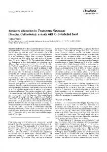
We propose several modifications to the original RAD design, which are later tested in simulations. Most of these modifications are generic, and can be applied to other ICA designs. Dynamic Minimum Increment calculates a minimum increment for each item and in each round separately depending on the competition rather than using fixed minimum increment through the auction and for all items. Higher minimum increment while competition is high can advance the auction faster, while lower increment when only a few bidders are left shall guarantee good price granularity. Consequently this rule shall reduce auction duration without sacrificing the efficiency. Figure 1 illustrates the model for price increment calculation, which we adopted after several design iterations. The x-axis indicates the number of bidders holding bids that contain the item in question, and the y-axis shows the corresponding increment value. Compared to a single minimum increment value in the RAD auction design, several parameters must be defined by the auctioneer in this case. The value of minIncrement determines the minimal minimum increment value, which is used when no competition (zero or one bidders) exist on the item. The value of maxIncrement is the maximal possible minimum increment value

might certainly get more valuable as the auction progresses. However this shall not invalidate previously submitted bids. In case the rule is still seen as too restrictive by bidders, it is possibly to make non-winning bids revocable. Besides the expected positive effect on allocation efficiency the rule also comes with a serious drawback. Keeping all bids active blows up the size of the winner determination. Hence, once the rule is active, the size of feasible auctions scenarios, i.e. the manageable number of items and bidders, can get reduced.

Figure 1. Dynamic minimum increment for an item. The value X defines minimal number of active bidders, required to reach the maxIncrement value. Especially important for auctions with small number of bidders is the curvature parameter (> 0). The calculation is performed by interpreting the points (1, minIncrement) as (0, 0) and (|X | , maxIncrement) as (1, 1) and then applying the power function xcurvature . Having different minimum increments on different items can certainly become too complex for bidders. This complexity, however, can easily be reduced by implicitly including the minimum increments into announced item prices for each round. Bundle Minimum Increment applies minimum increment not to each item in the bundle as defined by the RAD design, but to the bundle as a whole. Suppose the minimum increment value is set to 5 and we are interested in bundle (ABC). Under RAD rules, the bidder would be requested to bid 15 above ask price, 5 for each item in the bundle. Using Bundle Minimum Increment, a single increment of 5 would be applied to the whole bundle. This approach favors bids for big bundles. Old Bids Active rule implies keeping the bids from all rounds active throughout the auction. As straightforward optimization, we keep active only highest bid for each bidder and bundle. Having higher number of bids (and, thus, better information about bidders’ valuations) available for Winner Determination in late rounds of the auction shall help to find a more efficient allocation. The fact that bidders submit bids on bundles provides evidence that they are interested in the respective item combinations at given bid prices. This interest shall a priori not decline over time. Sooner or later, other item combinations

Last-and-Final Bids rule is inspired from the iBundle auction format outlined in [13]. It shall reduce efficiency losses in situations where price increment steps are too high for some bidders. Bidders are allowed to bid below the market price if following conditions are met: • Bid price is between the current ask price for the bundle (without the minimum increment) and the minimum bid price for the bundle (ask price plus minimum increment). • The bid is explicitly marked as last-and-final. For each bundle S and each bidder i, only one last-and-final bid is allowed. No further bids are accepted from bidder i for bundle S. Generally, higher minimum increment reduces the auction duration, but are more likely to result in efficiency losses due to high price granularity. Last-and-final bids can help to find a better compromise since bidders are allowed to bid between increment steps. Therefore this rule can potentially yield a faster auction progress without sacrificing the efficiency. Further advantage of this rule is the perceived fairness for the auction design on the bidder side, as they always have a possibility to bid their valuation. Forced Price Monotonicity is a simple way to ensure that prices do not fall throughout the auction. For each item, we compare newly calculated prices in round t with previous t − 1 round price. If the new price is lower, it is set to the level of round t − 1. Relaxed Eligibility. In some cases, especially when items in the auction significantly vary in price, bidders may want to replace a single expensive item by a set of cheaper items in their bids. Eligibility rules present a serious problem in this case. We introduce the notion of a surplus-eligibility, which allows a bidder to extend his eligibility and still stimulates competitive bidding. Surplus-eligibility SEit gives each bidder i a chance to increase his round t eligibility Eit . To retain the original pur-

pose of enforcing activity in the auction, size of the surpluseligibility is directly bound to the bidder’s market activity in the auction so far. The surplus-eligibility SEit for each bidder is calculated by the auction in each round and is communicated to the bidders along with prices and provisional allocation. In round t a bidder is allowed to bid - at maximum - on as many distinct items as he bid in the last round, plus surplus eligibility: Eit ≤ Eit−1 + SEit To determine the value SEit we need to find a fair measure for bidder’s market activity. An important concern is to avoid situations where bidders can artificially simulate activity by submitting deliberately loosing bids. We introduce the notion of bid volume of bidder i in round t. RBVit

=

X

maxbidpriceti (k) (Round Bid Volume)

k∈K

T BVi

=

T X

RBVit

(Total Bid Volume)

t=1

Function maxbidpriceti (k) determines the maximum bid price for the single item k based on bidder i’s bids in round t. For each bid bti (S), the price for all k ∈ S is determined by splitting the bundle bid price to individual items proportionally to item ask prices. For each item, the maximum over all bids value is taken. In other words, maxbidpriceti (k) figures out how much item k is maximally worth to bidder i in round t. The total bid volume T BVi equals the sum of RBVit over all auction rounds and represents the overall bid volume that bidder i generated in the auction so far. Further bidders are ranked by their T BVi in ascending order. The rank for bidder i, denoted by ri , is the index of the position in the ordered sequence of this bidder’s T BVi minus 1. The surplus eligibility is then calculated as:    ri t · SEmax SEi = round |I| − 1 ri The value |I|−1 lies in the range [0, 1] and represents the market activity factor. SEmax is the maximal surplus eligibility defined by the auctioneer. Summing up bidder activity through the whole auction rather then using only RBVit in determination of SEit ensures that bidders are stimulated to bid competitively right from the start of the auction.

4

Setup for Numerical Experiments

We have developed a generic simulation framework for ICAs including three main components: Value Models, Bidding Agents and Auction Processors.

Value Model generates valuations for all possible bundles for each bidder based on realistic, economically motivated scenarios. We have based our implementation on the Combinatorial Auctions Test Suite (CATS) that has been widely used for evaluation of winner determination algorithms [11]. In addition, we have used the Pairwise Synergy value model from [1]. Three different value model types were used. The Transportation value model is built following the idea of the Paths in Space model from CATS [11] with necessary adjustments for use in simulations of iterative CAs. It models a nearly planar transportation graph, where each bidder is interested in securing a path between two randomly selected vertices (cities). The items traded are edges (routes) of the graph. The Airport value model is an implementation of the Matching scenario in CATS with necessary modifications. It models four airports each having a predefined amount of starting and landing time slots. Each bidder is interested in obtaining one starting and one landing slot in two randomly selected airports. The bidder valuation is proportional to the distance between the airports, but can be reduced if the plane arrives later as planned or/and has to delay landing until the landing slot becomes available. The Pairwise Synergy value model is a slightly modified implementation of the model described in [1]. It is defined by a set of valuations of individual items and a matrix of pairwise item synergies (complementarities). A synergy value of 0 corresponds to completely independent items, and the synergy value of 1 means that the bundle valuation is twice as high as the sum of the individual item valuations. The model parameters are the interval for the randomly generated item valuations and the interval for the randomly generated synergy values. Bidding Agent implements a bidding strategy adhering to the given value model and to the restrictions of the specific auction design. We use powerset bidders, who always bid the minimal allowed price on all possible bundles that provide positive payoff at the current ask prices. It was not possible to use the myopic best response agent mainly because of the RAD eligibility rule. Myopic bidder usually looses his eligibility in early stages of the auction, which in turn results in low efficiency. The powerset does not suffer from this problem, and shall therefore provide the upper bound for auction efficiency compared to any other bidder types. Auction Processor implements the auction logic, enforces auction protocol rules, calculates ask prices and provisional allocation for the current round. Maximum surplus eligibility was set to 5, minimum increment curvature to 2, minimum number of bidders for

maximum increment to 5. Each of the new rules is analyzed separately on 70 auction samples for each of the following five value models:

Dynamic Minimum Increment rule has shown very good results in reducing auction duration. There were no noticeable changes to any other auction parameters.

• Airport value model with 84 items and 20 bidders.

Bundle Minimum Increment did not bring any improvements in auction outcome. Measurements do not show any common trend across all value models in any parameter. Furthermore Bundle Minimum Increment rule has some undesired side effects. We have measured significantly higher deviation between samples compared to the original RAD auction. Price calculation exhibits non-intuitive behavior, which can be perceived unfair from the bidders holding the bids on the higher priced bundles.

• Pairwise Synergy High value model with 7 items valued from 0 to 88, synergy values from 1.5 to 2.0, and 5 bidders with maximum bundle size of 4. • Pairwise Synergy Low value model with 7 items valued from 0 to 195, synergy values from 0 to 0.5, and 5 bidders with maximum bundle size of 4. • Transportation Large value model with 50 items (34 cities, edge density 2.9), average shipping utility 5.0, 30 bidders. • Transportation Small value model with 25 items (15 cities, edge density 3.2), average shipping utility 5.0, 15 bidders.

5

Simulation Results and Interpretation

This chapter presents simulation results for each of the proposed in Section 3 improvements, and analyzes the obtained data. Table 1 in Appendix summarizes all numbers obtained during simulations, Table 2 presents results of paired t-tests. Stars indicate positions, where significant difference between plain RAD and RAD with applied improvement was found. Old Bids Active rule is clearly the most effective way to increase auction efficiency out of all tested improvements. We obtain results of roughly 99% for each of the five value models. We explain the efficiency increase by higher number of bids available for winner determination in late rounds. Another positive impact of this rule is increased price monotonicity. However there is a significant reduction of the bidder’s revenue share too. Final prices are too high compared to minimum CE prices. Being aware of this auction property, real bidders can become conservative and never bid up to their valuations, which can negatively affect the auction’s efficiency. This phenomena however cannot be measured using our software bidders. Last-and-Final Bids had limited effect on most auction parameters. It can still be used to raise bidders’ fairness perception towards the auction. On the other hand, it is questionable if the rule is not too complex for bidders to understand and use.

Forced Price Monotonicity rule made prices fully monotonic. Another positive effect was slight reduction of auction duration. However auction efficiency has suffered losses, in some cases significant. Surplus Eligibility relaxes limitations on amount of different items in bids and consequently improves the efficiency. We have included the none-eligibility option in simulations which allows bids on any number of items independent of bid history. This rule is not practical since real bidders will misuse it and will not actively bid from first auction rounds. Our software bidders however bid competitively during the whole auction. Therefore the noneeligibility option gives the upper bound to the efficiency gain by a relaxed eligibility rule. Results show increased efficiency, significant in some cases. Most part of the gained efficiency goes to the auctioneer, bidders’ revenue is even decreased in some cases. However there is still potential upwards for surplus-eligibility, or other replacement for the activity rule, of up to roughly 1%. Summarizing analysis of suggested improvements, following list shows those rules which improve auction results. For each rule, we state its primary contribution. • Old Bids Active boost auction efficiency. • Last-and-Final bids have only slight positive effect on efficiency, but can increase bidders’ fairness perception towards the auction. • Dynamic minimum increment drastically reduces the number of auction rounds. • Surplus-eligibility increases auction efficiency. The forced price monotonicity rule was discarded due to its negative impact on the efficiency. The bundle minimum increment was not considered further either. We have conducted another set of simulations to test auction performance with all selected rules enabled. As the Old

Bids Active rule can imply limitations on the auction size, we have created two settings. First we include only three rules: Last-and-Final Bids, Dynamic Minimum Increment and Surplus Eligibility. Then we repeat simulations with all four rules enabled, including Old Bids Active. Tables 1 and 2 refer to results of these tests as Full excluding Old Bids Active and Full including Old Bids Active respectively. Results shows that already the Full excluding Old Bids Active setup improves auction results along many parameters significantly. The Full including Old Bids Active setup performs even better and reaches 99% efficiency for all value models. Both settings achieve significant reduction of auction duration and price fluctuations.

6

Conclusion and Outlook

In this paper we present a set of new rules for Iterative Combinatorial Auctions. We use numerical experiments to analyze their impact on the auction outcome based on our implementation of the RAD auction format. Results indicate significant improvements in several important parameters, including allocative efficiency and auction duration. We discuss practical applicability of the new rules and suggest possible combinations. Our future plans include analysis of the suggested rules using laboratory experiments with human bidders. We also want to continue looking for ICA improvements, and to study applicability and effect of different rules under varying conditions (value models, bidder strategies, etc.)

7

Glossary

K = {1, . . . , m} - set of items k ∈ K, also l - index for items I = {1, . . . , n} - set of bidders i ∈ I, also j - index for bidders S ⊆ K - bundle (package) vi (S) - valuation of the bidder i for the bundle S p(S) - anonymous bundle ask price of the bundle S p(k) - anonymous linear ask price of the item k P = {p(S)} or P = {p(k)} - set of ask prices B t = {bti (S)} - set of bids (bid prices) in the round t b ∈ B t - index for bids X = {xi (S)} - allocation X ∗ = {x∗i (S)} - efficient allocation

References [1] N. An, W. Elmaghraby, and P. Keskinocak. Bidding strategies and their impact on revenues in combinatorial auctions. Journal of Revenue and Pricing Management, 2005.

[2] L. Ausubel and P. Milgrom. The lovely but lonely vickrey auction. In P. Cramton, Y. Shoham, and R. Steinberg, editors, Combinatorial Auctions. MIT Press, Cambridge, MA, 2006. [3] S. Bikhchandani and J. M. Ostroy. The package assignment model. Journal of Economic Theory, 107(2):377–406, 2002. [4] P. Carlsson and A. Andersson. A flexible model for treestructured multi-commodity markets. Technical Report 2004-045, Uppsala University, Uppsala, Sweden, 2004. [5] P. Cramton, R. McMillan, P. Milgrom, B. Miller, B. Mitchell, D. Vincent, and R. Wilson. Simultaneous ascending auctions with package bidding. Report to the federal communications commission, Charles River and Associates, 1998. [6] P. Cramton, Y. Shoham, and R. Steinberg, editors. Combinatorial Auctions. MIT Press, Cambridge, MA, 2006. [7] M. Dunford, K. Hoffman, D. Menon, R. Sultana, and T. Wilson. Testing linear pricing algorithms for use in ascending combinatorial auctions. INFORMS Journal on Computing, to appear. [8] Y. Fujishima, K. Leyton-Brown, and Y. Shoham. Taming the computational complexity of combinatorial auctions: Optimal and approximate approaches. In International Joint Conference on Artificial Intelligence (IJCAI), Stockholm, Sweden, 1999. [9] T. Kwasnica, J. O. Ledyard, D. Porter, and C. DeMartini. A new and improved design for multi-objective iterative auctions. Management Science, 51(3):419–434, 2005. [10] D. Lehmann, R. Mueller, and T. Sandholm. The winner determination problem. In P. Cramton, Y. Shoham, and R. Steinberg, editors, Combinatorial Auctions. MIT Press, Cambridge, MA, 2006. [11] K. Leyton-Brown, M. Pearson, and Y. Shoham. Towards a universal test suite for combinatorial auction algorithms. In ACM Conference on Electronic Commerce, pages 66–76, 2000. [12] D. Mishra and D. Parkes. Ascending price vickrey auctions for general valuations. Journal of Economic Theory, forthcoming, 2006. [13] D. Parkes. Iterative Combinatorial Auctions: Achieving Economic and Computational Efficiency. PhD thesis, University of Pennsylvania, 2001. [14] D. Parkes and L. H. Ungar. Iterative combinatorial auctions: Theory and practice. In 17th National Conference on Artificial Intelligence (AAAI-00), 2000. [15] A. Pikovsky and M. Bichler. Information feedback and decision support in interative combinatorial auctions. In Wirtschaftsinformatik 2005, pages 329–348, Bamberg, Germany, 2005. Springer. Also available at http://ibis.in.tum.de/staff/pikovsky/index.htm. [16] M. H. Rothkopf, A. Pekec, and R. M. Harstad. Computationally manageable combinatorial auctions. volume 44, pages 1131–1147, 1998. [17] T. Sandholm and C. Boutilier. Preference elicitation in combinatorial auctions. In P. Cramton, Y. Shoham, and R. Steinberg, editors, Combinatorial Auctions. MIT Press, Cambridge, MA, 2006.

hhhh hhh Model hhValue hhh ICA Design hh h

RAD

Old Bids Active

Last and Final

Dynamic Minimum Increment

Bundle Minimum Increment

Forced Price Monotonicity

Surplus Eligibility

None Eligibility

Full excluding Old Bids Active

Full including Old Bids Active

∅ Efficiency ∅ Rev. Auctioneer ∅ Rev. Bidders ∅ Rounds ∅ Monoton. Error ∅ Efficiency ∅ Rev. Auctioneer ∅ Rev. Bidders ∅ Rounds ∅ Monoton. Error ∅ Efficiency ∅ Rev. Auctioneer ∅ Rev. Bidders ∅ Rounds ∅ Monoton. Error ∅ Efficiency ∅ Rev. Auctioneer ∅ Rev. Bidders ∅ Rounds ∅ Monoton. Error ∅ Efficiency ∅ Rev. Auctioneer ∅ Rev. Bidders ∅ Rounds ∅ Monoton. Error ∅ Efficiency ∅ Rev. Auctioneer ∅ Rev. Bidders ∅ Rounds ∅ Monoton. Error ∅ Efficiency ∅ Rev. Auctioneer ∅ Rev. Bidders ∅ Rounds ∅ Monoton. Error ∅ Efficiency ∅ Rev. Auctioneer ∅ Rev. Bidders ∅ Rounds ∅ Monoton. Error ∅ Efficiency ∅ Rev. Auctioneer ∅ Rev. Bidders ∅ Rounds ∅ Monoton. Error ∅ Efficiency ∅ Rev. Auctioneer ∅ Rev. Bidders ∅ Rounds ∅ Monoton. Error

Airport 95.19% 80.44% 14.75% 58.49 0.82 98.83% 89.32% 9.51% 55.10 0.76 95.19% 79.57% 15.62% 54.90 0.78 94.60% 79.06% 15.55% 46.69 0.84 94.45% 79.55% 14.90% 67.46 0.69 93.40% 77.55% 15.85% 56.09 0 95.23% 81.39% 13.84% 58.41 0.83 96.63% 82.73% 13.89% 58.86 0.82 95.35% 82.53% 12.82% 42.76 0.82 99.73% 92.77% 6.97% 38.80 0.70

PairSyn high 96.56% 81.02% 15.54% 50.07 0.36 98.61% 86.66% 11.95% 50.84 0.12 96.17% 79.99% 16.18% 48.53 0.33 94.94% 81.56% 13.38% 15.80 0.39 97.17% 78.52% 18.65% 45.73 0.40 95.66% 79.82% 15.84% 45.74 0 96.13% 82.53% 13.59% 49.24 0.35 97.00% 83.91% 13.09% 49.36 0.31 95.91% 85.83% 10.08% 14.39 0.32 99.81% 90.45% 9.35% 12.84 0.07

PairSyn low 96.67% 79.41% 17.26% 51.96 0.38 99.30% 87.45% 11.85% 54.03 0.11 96.03% 78.98% 17.05% 50.64 0.31 96.67% 81.99% 14.68% 16.10 0.36 97.53% 80.14% 17.39% 38.13 0.36 96.20% 78.99% 17.21% 49.23 0 97.23% 82.24% 14.99% 52.13 0.34 97.21% 82.26% 14.95% 51.47 0.35 97.45% 84.76% 12.69% 15.10 0.32 99.64% 90.96% 8.68% 14.74 0.08

Transp. large 94.61% 61.04% 33.57% 31.39 0.76 98.77% 67.52% 31.25% 28.06 0.72 94.02% 60.54% 33.48% 30.60 0.75 95.02% 62.48% 32.54% 17.57 0.66 92.34% 60.07% 32.26% 40.30 0.69 93.11% 60.54% 32.57% 29.06 0 96.10% 63.36% 32.74% 29.81 0.77 97.14% 65.99% 31.15% 29.64 0.78 97.34% 69.23% 28.11% 18.01 0.71 99.26% 73.39% 25.89% 15.86 0.62

Table 1. Overall performance results of the improved auction rules

Transp. small 93.79% 58.48% 35.30% 41.19 0.70 98.92% 67.66% 31.26% 41.41 0.69 94.00% 58.95% 35.05% 40.21 0.69 92.76% 57.95% 34.81% 24.54 0.67 91.53% 59.90% 31.64% 42.47 0.63 91.05% 58.59% 32.46% 39.24 0 95.37% 63.09% 32.29% 38.30 0.71 95.60% 63.10% 32.50% 37.77 0.70 95.43% 63.83% 31.61% 23.69 0.68 99.97% 75.01% 24.96% 28.91 0.63

hhhh

hhh Model hhValue Airport hhh ICA Design hh h Old Bids Act.

Last and Final

Dyn. Min. Inc.

Bundle Min. Inc.

Forced Price Mon.

Surp. Elig.

None Elig.

Full excl. OBA

Full incl. OBA

∅ Efficiency ∅ Rev. Auctioneer ∅ Rev. Bidders ∅ Rounds ∅ Monoton. Error ∅ Efficiency ∅ Rev. Auctioneer ∅ Rev. Bidders ∅ Rounds ∅ Monoton. Error ∅ Efficiency ∅ Rev. Auctioneer ∅ Rev. Bidders ∅ Rounds ∅ Monoton. Error ∅ Efficiency ∅ Rev. Auctioneer ∅ Rev. Bidders ∅ Rounds ∅ Monoton. Error ∅ Efficiency ∅ Rev. Auctioneer ∅ Rev. Bidders ∅ Rounds ∅ Monoton. Error ∅ Efficiency ∅ Rev. Auctioneer ∅ Rev. Bidders ∅ Rounds ∅ Monoton. Error ∅ Efficiency ∅ Rev. Auctioneer ∅ Rev. Bidders ∅ Rounds ∅ Monoton. Error ∅ Efficiency ∅ Rev. Auctioneer ∅ Rev. Bidders ∅ Rounds ∅ Monoton. Error ∅ Efficiency ∅ Rev. Auctioneer ∅ Rev. Bidders ∅ Rounds ∅ Monoton. Error

F F F F F

PairSyn high F F F F

PairSyn low F F F F F

Transp. large

Transp. small

F F F F F

F F F

F F F

F F

F F F

F

F F

F F F F F

F F

F F F

F F F

F

F

F F F F F F F

F F

F F

F F

F F

F F

F F

F

F F F

F F

F F

F F

F F F

F F

F F F F

F F F

F F F F F

F F F F F

F F F F F F F F F

F F F F F F F F F F F F F F F F F

Table 2. Results of paired t-tests for the improved auction rules

F F F F F F F F F F F F F F F F F F F