Saito distortion measure over the use of a fixed segmentation. 1. ... 2005 (the 2005 The first annual IEEE BENELUX/DSP Valley Signal Processing Symposium).
Proceedings of SPS-DARTS 2005 (the 2005 The first annual IEEE BENELUX/DSP Valley Signal Processing Symposium)
IMPROVED SUBSPACE BASED SPEECH ENHANCEMENT USING AN ADAPTIVE TIME SEGMENTATION Richard C. Hendriks, Richard Heusdens and Jesper Jensen {R.C.Hendriks, R.Heusdens, J.Jensen}@EWI.TUDelft.nl Delft University of Technology, Dept. of Mediamatics, 2628 CD Delft, The Netherlands ABSTRACT Subspace based speech enhancement relies on the decomposition of the vector space spanned by the covariance matrix of noisy speech into a noise subspace and a signal subspace, where the noise subspace is nulled and the signal subspace is modified by applying a gain function. This gain function is determined by the eigenvalues of the noise and noisy speech covariance matrix that are typically estimated from the noisy data using a fixed segmentation. A fixed segmentation often leads to covariance matrix estimates with an unnecessary high variance or a bias, because segments are shorter or longer, respectively, than the region where the noisy data is stationary. To overcome this problem we present an adaptive time-segmentation algorithm combined with subspace based speech enhancement. As a result, smearing of speech sounds and musical noise in the enhanced speech signal are reduced. Experiments show improvements in terms of segmental SNR of 0.6 dB and symmetrical ItakuraSaito distortion measure over the use of a fixed segmentation. 1. INTRODUCTION The growing interest for mobile speech communication systems over the last years also increased the demand to make those systems work with acceptable speech quality in acoustically noisy environments. Removing noise from speech signals before further processing (e.g. by a speech coder or recognizer) is one way to accomplish this. Because of their general applicability, single microphone speech enhancement techniques are often used to enhance the quality of speech signals degraded by noise. These techniques often assume additive noise models, e.g. y = x + n, with y the noisy speech, x the clean speech and n the noise process and furthermore that noise and speech are uncorrelated. The class of short-time Fourier transform (STFT) enhancement approaches have received significant interest over the last years [1, 2], because of their relatively good performance and low complexity. However, in general, STFT enhancement methods lead to introduction of an unnatural sounding residual noise, often referred to as musical noise. To reduce the amount of musical noise, smoothing methods like the decision directed approach [2] are often utilized. More recently, subspace based approaches [3] were introduced and have gained increased interest. In the basic formulation, The research is supported by Philips Research and the Technology Foundation STW, applied science division of NWO and the technology programme of the ministry of Economics Affairs.
the subspace based approach relies on an additional assumption of white noise. However, various methods have been presented that extend the subspace based approach to colored noise cases (e.g. [3, 4]). The idea of subspace based speech enhancement is to decompose the vector space spanned by the covariance matrix of the noisy speech signal into a signal subspace and a noise subspace. The signal subspace contains components of the clean signal as well as the noise process, while the noise subspace contains noise components only. Enhancement of noisy speech is performed by first transforming the noisy speech frame by frame using a Karhunen-Lo`eve transform (KLT). Then the noise subspace is nulled and the signal subspace is modified by applying a diagonal gain matrix G on the noisy KLT coefficients followed by an inverse KLT transform. We find the matrix G by, min kx − Hyk22 , H
with H = U GU # and U the KLT transform. This then leads to � G = I − diag σn2 /λy1 , ..., σn2 /λyk . (1) Here I is the identity matrix, σn2 the noise variance and λyk the eigenvalues of the noisy speech covariance matrix Ry . This implies exact knowledge of the second order statistics of the noisy speech and the noise. However, in practice exact knowledge of Ry is not available and therefore estimation of the covariance matrix is necessary. Estimates of Ry can be obtained using ˆy = R i
1 2T K
(i+T −1)K
X
Yn Yn# ,
(2)
n=(i−T −1)K+1
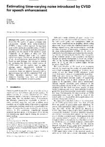
with Yn a K-dimensional vector of noisy speech samples starting at sample n, i the frame number for which the covariance matrix is estimated and T the number of frames from the past and the future used in the estimation of Ry . In order to apply (2) a segment of noisy speech is chosen from which Ry is estimated. Each segment may consist of a number of frames including the frame to be enhanced, as shown in Fig. 1. In [3], T was fixed at T = 5, leading to segments with a length of 11 frames. However, to get good estimates of Ry all vectors Yn must be chosen from stationary segments. Ideally, segments should vary with speech sounds: some vowel sounds may be considered stationary up to 40-50 ms, while stop consonants may be stationary for less than 5 ms [5]. However, typically a fixed segment size is used, which has two potential drawbacks. First, in signal regions which can be considered stationary for longer time than the segment used, the variance of the covariance estimator is unnecessarily large. This results in a larger variance
163
Proceedings of SPS-DARTS 2005 (the 2005 The first annual IEEE BENELUX/DSP Valley Signal Processing Symposium)
2T+1 frames
frame to be enhanced
1
segment
ˆ 1 [0] ∈ Rn0 and R ˆ 2 [0] ∈ RN −n0 be vectors containing Let R n0 (iid) realizations of R1 and N − n0 (iid) realizations of R2 , h iT ˆ 12 [0] = R ˆ 1 [0]T , R ˆ 2 [0]T respectively and let R ∈ RN . The
decision between the two hypotheses is made using the likelihood ratio test (LRT) [7],
0.5 0
Reject H0 if
−0.5 −1
R
ˆ 12 [0]|H1 ) p(R > γ, ˆ p(R12 [0]|H0 )
(3)
y
2.92
2.94
2.96 2.98 3 time samples (fs = 8000 Hz)
3.02
3.04 4
x 10
Figure 1: Noisy speech signal with frame to be enhanced. In this example a segment consists of 5 consecutive frames. of the estimated eigenvalues and, consequently, a larger variance of the gain function leading to an increased amount of musical noise. Secondly, if stationarity of the speech sound is shorter than this fixed segment size, Ry is estimated across stationarity boundaries resulting in a biased covariance matrix estimate. This leads to blurred speech sound transitions in the enhanced speech signal. In this paper, we propose to overcome the above mentioned shortcomings by combining subspace based speech enhancement with an adaptive time segmentation algorithm as described in [6]. The adaptive time segmentation determines a segment that reflects how many terms and which terms should be used within the covariance estimator. The combination of an adaptive time segmentation and the subspace speech enhancement approach leads to reduced musical noise because of a smaller variance of the covariance matrix. Further it leads to a reduced amount of speech distortions because transitions between speech sounds are better taken care of.
ˆ 12 [0]|H0 ) and p(R ˆ 12 [0]|H1 ) with γ a decision threshold, and p(R ˆ 12 [0] under hypoththe probability of observing the sequence R esis H0 and H1 respectively. From the assumption of independent frames it then follows that ˆ 12 [0]) = p(R ˆ 1 [0])p(R ˆ 2 [0]), p(R ˆ 1 [0]) = Qn+n0 −1 p(R ˆ 1i [0]) p(R i=n Q n+N −1 j ˆ ˆ 2 [0]) = and p(R j=n+n0 p(R2 [0]). We will argue that under ˆ 1i [0]) and p(R ˆ j [0]) are Gauscertain assumptions the pdfs p(R 2 sian and use the standard procedure of the Generalized LRT [7] and substitute unknown pdf parameters with their maximum likelihood estimates. ˆ i [0] 2.1. Distribution of R The central limit theorem states that the normalized sum of a large number of mutually independent random variables with zero means and finite variances tends to the normal probability distribution provided that the variances σk2 , k = Pindividual 2 1, ..., L are small compared to L σ [8]. To determine the k=1 k ˆ i [0] we assume that the time samples are distribution type of R independent random variables (as is commonly done in speech enhancement [9]). Because Ri [0] can be estimated as L X ˆ i [0] = 1 R y 2 (k), L k=1
2. ADAPTIVE TIME SEGMENTATION The segmentation algorithm we propose here is based on a probabilistic framework, where segments are formed based on the outcome of a hypothesis test. We test the hypotheses whether two wide sense stationary consecutive sequences of time-samples can be merged to form one segment or not. Here we regard sequences of time samples as an outcome of random process Y and search for sequences that are stationary to a certain degree. In particular, we will use a test statistic based on a necessary condition for stationarity, namely that zero-lag correlation coefficients of the random process �must remain invariant over time. This means that R[0] = E |Y|2 , with R[0] the correlation coefficient with lag 0, should be constant over time. Let s1 and s2 be two neighboring wide sense stationary segments, both consisting of independent frames with frame numbers i ∈ {n, ..., n + n0 − 1} and j ∈ {n + n0 , ..., n + N − 1} ˆ 1i [0] and R ˆ j [0] denote estimates of R[0] respectively, and let R 2 ˆ 1i [0] and R ˆ j [0] as realizafor each such frame. We can view R 2 tions of random variables R1 and R2 , respectively. The two hypotheses then are: H0 : H1 :
R1 and R2 have the same distribution ( [s1 , s2 ] is considered stationary) R1 and R2 do not have the same distribution ( [s1 , s2 ] is not stationary),
ˆ i [0] is a sum of independent random variables and it follows R ˆ i approaches a Gaussian distribution. Knowing then that R[0] ˆ i [0], we are now in a position to compute the distribution of R the likelihood ratio given in Eq. (3). ˆ i [0], we To verify the above assumed Gaussian distribution of R ˆ i [0] show in Figure 2 a comparison between a histogram of R measured from a synthetic noisy speech signal, and a Gaussian distribution whose mean and variance are estimated from the noisy data. The synthetic speech signal was created by filtering an impulse train through a time-invariant LPC-synthesis filter whose coefficients were extracted from a speech signal. The pdf was measured by windowing the noisy speech data followed ˆ i [0] per window. by computation of R 2.2. Segmentation Procedure In principle, to find for a given frame a corresponding segment, we should perform an exhaustive search over all possible segments. To avoid this computationally demanding full-search approach, we propose instead a computationally simpler algorithm which simulation experiments have shown to lead to the same performance as the full search algorithm. In Fig. 3 this simplified algorithm is described. Start with a minimum segment s1 , which is assumed to be stationary and contains the frame under consideration (shaded area in Fig. 3). Then extend this
164
Proceedings of SPS-DARTS 2005 (the 2005 The first annual IEEE BENELUX/DSP Valley Signal Processing Symposium) 0.9
assumed Gaussian pdf measured pdf
0.8 0.7 0.6 0.5 0.4 0.3 0.2 0.1 0 2
3
4
5
6
7
8
9
10
11
12
1500
ˆ i [0]. Figure 2: Measured distribution of R
2000 2500 time samples (fs = 8000 Hz)
3000
Figure 4: Example Segmentation. Thick horizontal lines: Duration of frames. Thin horizontal lines: Corresponding segments. s1 s2 accept H0
s2 accept H0
s1 s1
covariance matrix estimation from Eq. (2) then leads to
s2 accept H0
s2
ˆy = R i
accept H0
s1
s2 reject H0
s2 accept H0 reject H0
s2
1 (T1 + T2 )K
(i+T2 −1)K
X
Yn Yn# ,
(4)
n=(i−T1 −1)K+1
where T1 and T2 are determined by the segmentation algorithm.
s1
3. EXPERIMENTAL RESULTS
s1 s1 time
Figure 3: Segmentation algorithm based on hypothesis.
minimum segment with one frame at a time in an iterative process. Whether the segment should be extended with a neighboring frame is decided using the hypothesis test over sequence s 1 and a neighboring sequence s2 . We continue this process until on both sides of s1 H0 is rejected. The final sequence s1 is considered as the stationary segment that can be used for smoothing of the noisy speech power spectrum. In Fig. 4 we show the result of the above described hypothesis based segmentation algorithm applied to a speech signal degraded by white noise at an SNR of 15 dB. In the figure the original clean speech signal is shown together with the resulting segmentation. The thick lines mark the frames in which the signal is divided for enhancement. The thin lines represent for each frame the corresponding segment that is found by the hypothesis based algorithm. The speech signal under consideration consists of four parts. An initial silence part, a transient, ringing after the transient and a voiced part. We see that frames in the silence and voiced part have long segments associated which cover respectively the whole silence and voiced part. Frames in the transient part have rather short segments. This prevents smearing of the transient. Further the beginning of the voiced part is resolved, preventing it from smearing into the ringing of the transient. Combining this adaptive time segmentation algorithm with the
The presented segmentation algorithm is evaluated by means of objective experiments. In all experiments the fragments were sampled at 8 kHz. Frame sizes of 120 samples with 50 percent overlap were used. We use the segmentation algorithm as a front-end for a subspace based enhancement algorithm with a gain function as in Eq. (1), where the eigenvalues are determined with the covariance estimator in (4) and the one in (2), respectively. The rank of the signal subspace was estimated as in [3]. Noisy speech signals are constructed by adding white Gaussian noise to clean speech signals. In Fig. 5 the impact of our segmentation algorithm is demonstrated on a male speech signal. The SNR per frame using subspace based speech enhancement combined with an adaptive time segmentation is compared with subspace based enhancement with a fixed segmentation. Further, the original clean speech signal is shown. For the fixed segmentation with T = 5, and for the adaptive time segmentation the threshold γ is chosen to γ = 108.7 , both leading to optimal segmental SNR. SegmenPN −1 kxi k2 , with N the tal SNR is defined as N1 i=0 10 log10 kxi −ˆ x i k2 number of frames [5]. The clean speech signal was degraded with white noise at an SNR of 10 dB. Performance improvements are especially present where the clean speech signal shows abrupt changes like transitions between speech sounds, which means less smearing of speech sounds. In order to evaluate the objective quality we apply two different objective quality measures, namely the averaged segmental SNR and the symmetrical Itakura-Saito distortion measure (IS) [10]. Fig. 6 and Fig. 7 show the average segmental SNR and the average symmetrical Itakura-Saito distortion measure, respectively, as a function of the input SNR, for subspace based
165
Proceedings of SPS-DARTS 2005 (the 2005 The first annual IEEE BENELUX/DSP Valley Signal Processing Symposium) 25
35
Enhanced with adaptive segmentation Enhanced with fixed segmentaton
20
30 sym. Itakura−Saito (dB)
15 10 SNR (dB)
Enhancement with adaptive segmentation Enhancement with fixed segmentation Noisy
5 0 −5
25
20
15
−10 −15 7000
7500
8000
8500 9000 9500 time (samples)
10000
10500
11000
Figure 5: SNR per frame after enhancement with subspace approach based on adaptive time segmentation (solid) and subspace approach based on fixed time segmentation (dotted). 8
seg. SNR (dB)
6
10 5
10 Input SNR
15
Figure 7: Objective performance in terms of symmetrical Itakura-Saito distortion measure versus input SNR. that the proposed scheme improves over the more conventional fixed segmentation.
Enhancement with adaptive segmentation Enhancement with fixed segmentation Noisy
4
5. REFERENCES
2
[1] S. F. Boll, “Suppression of acoustic noise in speech using spectral subtraction,” IEEE Trans. Acoust., Speech, Signal Processing, vol. ASSP-27, no. 2, pp. 113–120, April 1979. [2] Y. Ephraim and D. Malah, “Speech enhancement using a minimum mean-square error short-time spectral amplitude estimator,” IEEE Trans. Acoust., Speech, Signal Processing, vol. ASSP-32, no. 6, pp. 1109–1121, December 1984. [3] Y. Ephraim and H. L. van Trees, “A signal subspace approach for speech enhancement,” IEEE Trans. Speech Audio Processing, vol. 3, no. 4, pp. 251–266, July 1995. [4] H. Lev-Ari and Y. Ephraim, “Extension of the signal subspace speech enhancement approach to colored noise,” IEEE Signal Processing Letters, vol. 10, no. 4, pp. 104– 106, April 2003. [5] J.R. Deller, J. H. L. Hansen, and J. G. Proakis, DiscreteTime Processing of Speech Signals, IEEE Press, Piscataway, NJ, 2000. [6] R. C. Hendriks, R. Heusdens, and J. Jensen, “Adaptive time segmentation of noisy speech for improved speech enhancement,” in IEEE Int. Conf. Acoust., Speech,Signal Processing, 2005. [7] H. L. van Trees, Detection, Estimation and Modulation Theory, vol. 1, John Wiley and Sons, 1968. [8] H. Stark and J.W. Woods, Probability, random processes, and estimation theory for engineers, Prentice-Hall, Englewood Cliffs, NJ, 1986. [9] Y. Ephraim and D. Malah, “Speech enhancement using a minimum mean-square error log-spectral amplitude estimator,” IEEE Trans. Acoust., Speech, Signal Processing, vol. 33, no. 2, pp. 443–445, April 1985. [10] A. H. Gray. Jr. and J. D. Markel, “Distance measures for speech processing,” IEEE Trans. Acoust., Speech, Signal Processing, vol. ASSP-24, no. 5, pp. 380–391, October 1976.
0
−2 −4 −6 −8 5
10 Input SNR (dB)
15
Figure 6: Objective performance in terms of averaged segmental SNR versus input SNR. speech enhancement combined with adaptive segmentation, subspace based speech enhancement combined with fixed segmentation and the unprocessed noisy speech signal. The results are averaged over six different signals with a duration of 3-4 seconds each. Fig. 6 shows an improvement in terms of average segmental SNR of approximately 0.6 dB across the range of input SNRs. This is consistent with the results of Fig. 7, where improvement in terms of symmetrical IS is shown for all input SNRs. Informal listening tests confirmed that with the adaptive time segmentation the transitions between speech sounds are sharper and less distorted. 4. CONCLUSIONS We presented an improved subspace based speech enhancement approach using an adaptive time segmentation. The proposed segmentation algorithm uses sequences of hypothesis tests to find a segment for a given frame. The segments are used within a subspace based enhancement algorithm to make better estimates of the covariance matrix that are then adapted to the underlying noisy speech signal. In terms of objective quality measures (segmental SNR and symmetrical IS distortion measure) it is shown
166