Improved Wind Power Forecasting with ARIMA Models

21st European Symposium on Computer Aided Process Engineering – ESCAPE 21 E.N. Pistikopoulos, M.C. Georgiadis and A. Kokossis (Editors) © 2011 Elsevier B.V. All rights reserved.

Improved Wind Power Forecasting with ARIMA Models Bri-Mathias Hodge, Austin Zeiler, Duncan Brooks, Gary Blau, Joseph Pekny, Gintaras Reklatis Purdue University School of Chemical Engineering, 480 Stadium Mall Dr., West Lafayette, IN 47907, United States

Abstract The introduction of large amounts of wind power into the electricity system raises potential reliability issues for the grid due to the intermittent nature of wind power. Wind power cannot be scheduled in advance like conventional generation units and thus forecasts of the wind power that will be produced in future hours are used to schedule the amount of wind power available. Any improvements in wind power forecasting have the potential to reduce the amount of reserves necessary in systems with significant amounts of wind power, and eventually lower the cost of electricity in such systems. In this work we examine the ability of statistical time series analysis tools, namely autoregressive integrative moving average (ARIMA) models, to forecast future wind power output from historical data. A systematic approach to determine the best values for the assortment of variables associated with the models, such as training period length and model orders, has been developed and applied. The ability of the models to outperform a standard forecasting benchmark has been examined at a number of different forecast period lengths. The application of the tools to total power output of the many wind farms that may be present within the territory of a single independent system operator is studied. Finally, a case study involving wind farm data from Ontario, Canada is used to show how the improvements that these statistical techniques offer may be beneficial for the independent system operator. Keywords: Energy systems modeling, Forecasting, Electricity Systems, Wind power

1. Introduction Wind power is the fastest growing renewable energy technology worldwide with nearly 10 GW of electricity production capacity installed in the United States alone in 2009 (American Wind Energy Association, 2010). Since wind power output is both intermittent and uncertain in nature, the introduction of large amounts of wind power capacity into the electricity system has the potential to disrupt normal operations where large thermal generation units must be scheduled as far as a day in advance. Since the wind cannot be controlled, the next best solution is to be able to forecast the wind output. While this does not eliminate the variability, it can reduce the uncertainty involved. Improvements in wind forecasting technology can reduce the amount of uncertainty in the system operation, necessitating lower amounts of spinning reserves and reducing overall system cost. Autoregressive integrative moving average (ARIMA) models are one method of statistical time series analysis to forecast wind future wind power output, and constitutes the approach that will be highlighted in this work. Typically, a wind forecast model is evaluated based on its improvement over the Persistence model. In the Persistence method, the previous value of the time series is

2

B-M. Hodge et al.

used as the forecast for the subsequent period. This simple approach serves as a baseline that any forecasting method must improve upon in order to be considered practically useful. Previous work in short-term wind power forecasting has focused on ARMA models that implicitly assume data stationarity (Milligan et al., 2003). A more thorough review of techniques for short-term wind forecasting is provided in (Lei et al. 2009). This work will focus on ARIMA models as a means for forecasting future wind power values in an attempt to outperform Persistence for one hour forecasts. There are a number of different parameters that can affect the utility of the ARIMA forecasting method, including training period length and model orders. We have attempted to apply as systematic of an approach toward the selection of these values as possible. We have chosen to focus on the problem encountered by a system operator, forecasting the combined power output of a number of wind farms together, instead of forecasting only a single turbine, or single wind farm, output. The data utilized in this study comes from simulated data supplied by the National Renewable Energy Laboratory (National Renewable Laboratory, 2009) and also real wind data from Ontario, Canada (Ontario Power Authority, 2010). These case studies are used to showcase the improvements that these statistical techniques may offer independent system operators, or large balancing authorities.

2. Data and Methods 2.1. Data Used One source of wind data used in the analysis is the Western Wind Integration Dataset of the National Renewable Energy Laboratory (National Renewable Laboratory, 2009). The dataset is comprised of simulated wind speed and power outputs for individual locations throughout the western United States. The production is sampled every 10 minutes for the years 2004 to 2006. Ten Vestas V90 3 MW wind turbines with a 100 meter hub height are hypothetically placed at each location to translate wind speed data into power output. A subset was constructed from the 650 California onshore sites with the highest average capacity factors for the years 2004-2006. The dataset used has a power capacity of 19.5 GW. The analysis uses data beginning January 1, 2006. While the NREL simulated data has been benchmarked to replicate the patterns of actual wind power output, a source of real data was also used to check the applicability of the results to real wind data. This data is from the Independent Electricity System Operator (IESO) of the Ontario Power Authority in Ontario Canada, which provides wind farm power production online (Ontario Power Authority, 2010). Ontario currently has eight wind farms in total, and the website is continually updated to show the previous 90 days of hourly production by wind farm. The total capacity of the wind farms is under 1.1 GW, a value considerably less than the 19.5 GW of simulated capcity from the NREL dataset. The analysis uses data from April 29 to August 1, 2010. 2.2. Forecasting Model Training While wind power can vary significantly within the hourly period, the hour timeframe is commonly used in power scheduling and dispatching work. Therefore, the NREL and Ontario datasets were analyzed at one hour intervals. The ARIMA model fitting and forecasting was performed using the R statistical software environment (Homik, 2010). An important consideration when dealing with time series data is the amount of training data provided. This length of time specifies the number of points up to the present to which the ARIMA model parameters for the model order will be fit. A range from 1

Improved Wind Forecasting with ARIMA Models

3

day to 30 days was tested by making 24 consecutive 1 hour forecasts using 18 different models. This analysis was performed for ten different randomly selected NREL locations. On average, the accuracy of the forecasts increased with the length of training period. A 30 day training period, however, may be impractical due to computation time limitations. A 14 day training period was selected based on its convenience as a calendar measure (2 weeks) and relative length. 2.3. Summed Data In order to find the best models to forecast the total summed production of the NREL dataset, a goodness of fit criteria was used. The Akaike Information Criterion (AIC) was chosen as the criteria by which to compare models. The AIC is a measurement of the tradeoff between the accuracy and complexity of a model, hence punishing overfitting. For the model selection process, 625 different ARIMA models were tested on the training data for the sum of the 650 NREL wind farm locations. The 20 models showing on average the best, or minimum, AIC results were used to forecast two weeks of hourly data. As mentioned previously, a model is evaluated based on its improvement upon the Persistence model. The error of each model was calculated using the Root Forecast Mean Square Error (RFMSE), and then that error was compared to the error of the Persistence method using the Persistence to Model Error Ratio (PMER). (1) Equation 1: Root Forecast Mean Square Error, where pt is the actual and ^pt the forecasted power

(2) Equation 2: Persistence to Model Error Ratio

2.4. Ensemble Forecasting of Summed Data Another method of forecasting was developed simply by taking the average forecasts of a number of models. This ensemble forecast was made using the five models showing the best PMER; the five forecasts were averaged and compared to the results of the models by themselves. 2.5. Combination of Models A further method of producing forecasts for the summed data was developed and tested. The idea of this method is to take a weighted average of the best performing individual model parameters and use those values to forecast the summed data. For example, with the NREL data, a given model forecasted the 650 individual wind farms using different parameters –values for p and q in the ARIMA(p, d, q) format. Each wind farm’s hourly forecast had an RFMSE, measuring the accuracy of the model’s prediction. The inverse of the RFMSE (the lower the value, the worse the model’s performance) was used to find a weighted proportion based on performance for each of the 650 wind farms. Then, the weighted proportion values were applied to the summation of the following hour forecasting parameters. This summation leads to the parameter used in the model (“combined” model) to forecast the summed NREL data.

4

B-M. Hodge et al.

(3) Equation 3: Weighted parameter using the model combination method, Where pweighted is the parameter used to forecast the summed NREL data, pk is the parameter for each individual wind farm, and RFMSEk/i are the RFMSEs of the prior hour’s forecast for each individual wind farm

The new RFMSE, inverse RFMSE and weights were calculated from the performances of the most recent individual parameters on the individual data and then the cycle was repeated for a forecast period of two weeks or 336 hours. The “combined” model RFMSEs were then compared to the Persistence model, as well as the other individual models that yielded the best results for the summed data.

3. Results and Discussion The five models with the best PMER results are shown along with the PMER of the ensemble forecast in Figure 1 below. The five best performing models for the NREL data forecasted approximately 20% better the Persistence model. These models, when applied to the real Ontario data, performed over 5% better than Persistence. Taking the average forecast of these models had a PMER nearly equal to that of the best performing models for both datasets. The best models for the NREL data were (1,2,2), (2,2,1) and the ensemble forecasts. And when applied to the Ontario data the best were (1,2,1), (2,2,1) and the ensemble.

Figure 1: The PMER results of the best performing models’ forecasts and the ensemble of the forecasts for the NREL and applied to the Ontario data

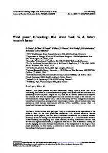
The five best “combined” models are shown below in Figure 2. The PMER scale is the same as Figure 1 to compare the performance of the models. When the “combined” models method was applied, the results for the NREL data were nearly universally equivalent to the Persistence model. The (3,1,1) model was the only one with a PMER over one. When the models were applied to the Ontario data, however, all performed approximately 5% better than Persistence. While the performance of the models was slightly worse when applied to the Ontario data, as opposed to the NREL data set for which the model orders were fitted, the fact that it still produced better results than Persistence is encouraging. Therefore, the models used for forecasting 19.5 GW of simulated capacity in a Californian winter can still be used for forecasting 1.1 GW of real capacity in an Ontario summer. The “combined” models method did not appear to add value, as the overall performance was

Improved Wind Forecasting with ARIMA Models worse than that of the original method. An interesting similarity between the best performing models is that the integrative term was two, meaning the wind power time series was non-stationary and the trends were linear. For the “combined” models the stationarity was third order. In any case, it seems that ARIMA models should be used over ARMA models (integrative term of zero) due to the non-stationarity of the data.

Figure 2: The PMER results of the best performing models using the "combined" method for the NREL data and applied to the Ontario data

4. Conclusion A systematic approach to determine the best values for the assortment of variables associated with ARIMA/ARMA models, such as training period length and model orders, has been developed and applied. The one hour forecasts of the models were compared to the Persistence model as a standard in order to deem the models’ effectiveness. Using the AIC criteria, a 14 week training period was chosen to balance computing time and relative error. The “combined” models method showed little promise in its PMER results. However the original method of using individual models for forecasting showed consistent improvement over Persistence, especially the models (2,2,1) and the method of taking the ensemble forecasts. These showed promise for the NREL wind data used and also when applied to Ontario data, an encouraging sign for ARIMA models’ adaptability between different weather climates and seasons. The improved forecasting results are useful as wind energy increasingly contributes power to the system and predicting production of this intermittent energy source becomes more vital to its growth with increasing wind power installed capacity.

References American Wind Energy Association, 2010, AWEA Year End 2009 Market Report K. Homik , 2010,The R FAQ [Online], [cited 2010 Aug 8], Available from: http://crean.rproject.org/doc/FAQ/R-FAQ.html M. Lei, L. Shiyan, J. Chuanwen, L. Honglin, Z. Yan, 2009, A Review on the Forecasting of Wind Speed and Generated Power, Renewable and Sustainable Energy Reviews, 13, 4, 915-920 M. Milligan, M. Schwartz, Y. Wan, 2003, Statistical Wind Power Forecasting Models: Results for U.S. Wind Farms, Proceedings of WINDPOWER 2003, Austin, Texas National Renewable Energy Laboratory, 2010, Wind Integration Datasets [Online], [cited 2010 Aug 23], Available from: http://www.nrel.gov/wind/integrationdatasets. Ontario Power Authority , 2010, Wind Power [Online], [cited 2010 Aug 8], Available from: http://www.powerauthority.on.ca/Page.asp?PageID=1212&SiteNodeID=234

5