system. (Thus, if a new genre emerges, everything needs to be recomputed.) The first .... on guitar chords and vocals, while the drums are hardly noticeable.
IMPROVEMENTS OF AUDIO-BASED MUSIC SIMILARITY AND GENRE CLASSIFICATON
1
Elias Pampalk1 , Arthur Flexer1 , Gerhard Widmer1,2 Austrian Research Institute for Artificial Intelligence (OFAI) Freyung 6/6, A-1010 Vienna, Austria 2 Department of Computational Perception Johannes Kepler University, Linz, Austria {elias,arthur,gerhard}@ofai.at
ABSTRACT Audio-based music similarity measures can be used to automatically generate playlists or recommendations. In this paper the similarity measure that won the ISMIR’04 genre classification contest is reviewed. In addition, further improvements are presented. In particular, two new descriptors are presented and combined with two previously published similarity measures. The performance is evaluated in a series of experiments on four music collections. The evaluations are based on genre classification, assuming that very similar tracks belong to the same genre. On two collections the improvements lead to a substantial performance increase. Keywords: Spectral Similarity, Fluctuation Patterns, Descriptors, Music Similarity, Genre Classification
1
INTRODUCTION
Music similarity computed from the audio signal can be applied to playlist generation, recommendation of unknown pieces or artists, or organization and visualization of music collections. Unfortunately, music similarity is very complex, multi-dimensional, context-dependent, and ill-defined. To evaluate algorithms which model the perception of similarity would require extensive listening tests. A cheaper alternative is to evaluate the performance in terms of genre classification. The assumption is that pieces very similar to each other belong to the same genre. We believe this assumption holds in most cases despite the fact that music genre taxonomies have several limitations (see e.g. [15]). An obvious issue is that many artists have a very individual mix of several styles which is often difficult to pigeonhole. Nevertheless, genres are a widely used concept to manage large music collections, and genre labels for artists are readily available. Permission to make digital or hard copies of all or part of this work for personal or classroom use is granted without fee provided that copies are not made or distributed for profit or commercial advantage and that copies bear this notice and the full citation on the first page. c
2005 Queen Mary, University of London
In this paper we review the algorithm, based on the work of Aucouturier and Pachet [2], which won the ISMIR’04 genre classification contest. Furthermore, we demonstrate how the performance can be improved. In particular, we combine spectral similarity (which describes aspects related to timbre) with fluctuation patterns (which describe loudness fluctuations over time) and two new descriptors derived thereof. To evaluate the results we use four music collections with a total of almost 6000 pieces and up to 22 genres per collection. One of these collections was used as training set for the ISMIR’04 genre classification contest. Using last years winning algorithm as baseline our findings show improvements of up to 41% (12 percentage points) on one of the collections, while the results on the contest training set (using the same evaluation procedure as in the contest) increased by merely 2 percentage points. One of our main observations is that not using different music collections (with different structures and contents) can lead to overfitting. Another observation is the need to distinguish between artist identification and genre classification. Furthermore, our findings confirm the findings of Aucouturier and Pachet [2] who suggest the existence of a glass ceiling which cannot be surpassed without taking higher level cognitive processing into account. The remainder of this paper is organized as follows. Section 2 covers related work. In Sect. 3 we discuss the audio-based similarity measures we use (and used for the contest) and present the two new descriptors. In Sect. 4 the experiments and results based on genre classification are presented. In Sect. 5 conclusions are drawn.
2
RELATED WORK
There is a significant amount of research on audio-based genre classification with one of the first approaches presented in [23]. More recent approaches include, for example [13, 24]. Most of these approaches do not focus on similarity measures (and do not use nearest neighbor classifiers to evaluate the performance). However, contentbased descriptors which work well for classifiers are also good candidates to be included in a similarity measure. An overview and evaluation of many of the descriptors used for classification can be found in [21]. In addition, recent work suggests that it is possible to automatically extract features [26].
3
AUDIO-BASED MUSIC SIMILARITY
In this section we review spectral similarity and present the parameters which won the ISMIR’04 genre contest. We review the fluctuation patterns from which we extract two new descriptors, namely “Focus” and “Gravity”. Furthermore we describe how we combine these different sources of similarity. The idea of combining fluctuation patterns and the descriptors with spectral similarity is to add complementary information. The reason for not using descriptors based on the overall loudness (or intensity) is because we have found these to be very sensitive to production effects (e.g. compression). Furthermore, we do not use spectral descriptors (e.g. spectral centroid) because these aspects are covered by the spectral similarity measure. 3.1
Spectral Similarity
Spectral similarity captures aspects related to timbre. However, important timbre characteristics such as the attack or decay of a sound are not modeled. The general idea is to chop the audio signal into thousands of very short (e.g. 20ms) frames and ignore their order in time. Each frame is described by its Mel Frequency Cepstrum Coefficients (MFCCs). The large number of frames is summarized by a model obtained by clustering the frames. The distance between two pieces is computed by comparing their cluster models. The first approach in this direction was presented by Foote [7], who used a global set of clusters for all pieces in the collection. The global set was obtained from a classifier. However, there are several disadvantages having global clusters. For example, it is only possible to describe music similar to the music already known to the system. (Thus, if a new genre emerges, everything needs to be recomputed.) The first localized approach was published by Logan and Salomon [10]. For each piece an individual set of clusters is used. The distances between these are computed using the Earth Movers Distance [22]. Aucouturier and Pachet improved this approach by using Monte Carlo sampling instead [1]. The implementations we review here are implemented in the MA Toolbox [17].
Amplitude
For our work the most important ingredient is spectral similarity based on Mel Frequency Cepstrum Coefficients [1, 2, 7, 10]. Similar audio frames are grouped into clusters which are used to compare pieces (we describe the spectral similarity in detail later on). For these similarity measures the focus in terms of applications is mainly on playlist generation and recommendation (e.g. [9, 11]). Alternatives include the anchor space similarity [4] and the fluctuation patterns [16, 18]. Not much work has been carried out to compare different similarity measures. First attempts were made in [5, 19]. In addition, related work includes approaches using cultural information retrieved from the web (such as playlists, reviews, lyrics, web pages) to compute similarity (e.g. [3, 8, 12, 14, 25]). These web-based approaches can complement audio-based approaches.
PCM Audio Signal 1 0 −1 10
20 30 Time [ms]
40
dB−SPL dB−SPL
FFT Spectrum 100
100
50 0 MFCCs (Decoded) 50 0
Sone
Sone 20 10 0 50
100 200 400 800 1600 3200 6400 Frequency [Hz]
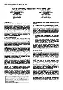
Figure 1: Different frame representations. The lower three plots have a logarithmically scaled x-axis. The dots in the MFCC and Sone plots depict the center frequencies of the bands. 3.1.1
MFCCs
Mel Frequency Cepstrum Coefficients are a very popular approach to represent the spectrum of an audio frame. Frame sizes are usually around 10-100ms. The MFCCs for each frame are computed in the following steps. First, the frequency domain representation is computed using a FFT. Second, the frequency bins are grouped into overlapping frequency bands (usually around 40). The widths and centers of the frequency bands are based on the non-linear Mel-scale. The scale is designed so that a tone with a certain Mel value is perceived twice as high as a tone with half the Mel value. Third, the amplitudes are transformed into a perceptual scale. Usually, the logarithm is computed (dB). Finally, a discrete cosine transform (DCT) is applied. From the obtained coefficients usually the first 20 are kept. This results in a spectrally smoothed and compressed representation. Figure 1 illustrates the difference between the spectral representation obtained from the FFT and the MFCCs. The primary difference is that the MFCC representation is much smoother. The second important difference is the change in the scaling of the frequency. 3.1.2
Frame Clustering
A three minute piece is represented by several thousand frames. Most of these represent reoccurring sounds such as an instrument or a voice. The goal of the frame clustering is to group similar frames together and describe each of these clusters by the mean and variance (using a diagonal covariance matrix). The number of clusters used ranges from 3-50. Several alternative clustering algorithms can be used for this task. Logan and Salomon suggest using kmeans [10] while Aucouturier and Pachet use Gaussian mixture models with expectation maximization [1]. As demonstrated in [2] the choice of the clustering algorithm is not a critical factor for the overall quality. However, computation times might be an issue.
Flex Brubeck et al. Spider Take Five
FP
Everlast Black Jesus
Spears Crazy
Beach Boys Surfin’ USA
CM
FP.F
FP.G
0.28
−6.4
0.16
−5.0
0.23
−6.4
0.32
−5.9
0.42
−5.8
Figure 2: Visualization of the features. On the y-axis of the cluster model (CM) is the loudness (dB-SPL), on the x-axis are the Mel frequency bands. The plots show the 30 centers and their variances on top of each other. On the y-axis of the FP are the Bark frequency bands, the x-axis is the modulation frequency (in the range from 0-10Hz). The y-axis on the FP.F histogram plots are the counts, on the x-axis are the values of the FP (from 0 to 1). The yaxis of the FP.G is the sum of values per FP column, the x-axis is the modulation frequency (from 0-10Hz). Examples of cluster models are given in Figure 2. All of the clusters models have little energy in high frequencies and lots of energy (with a high variance) in the low frequencies. As the cluster models are a very low-level representation it is difficult to guess the actual instrumentation by looking at the figures. 3.1.3
Cluster Model Similarity
Computing the similarity of two pieces of music given their cluster models is not as straightforward as distance computations in a vector space. Two approaches exist, one uses the Earth Movers Distance [10], the other Monte Carlo sampling [1]. The Earth Movers Distance computes the necessary “work” to transform one model into another. First, the distances between all clusters from one piece to all clusters from the other piece are computed using the KullbackLeibler divergence (taking the variances into account). Then, one piece is treated as supplier (with each cluster being a supply center with a capacity defined by the number of frames belonging to the cluster), the other piece as demander (and demand centers defined by the clusters). The minimum cost to transfer the frames defines the similarity of the pieces. Monte Carlo sampling means that the cluster models are treated as probability distributions from which samples are drawn. The sample size usually ranges from 200 to 2000. To compute the similarity of pieces α and β a sample from each is drawn, Sα and Sβ respectively. The log-likelihood L(S|M ) that a sample S was generated by the model M is computed for each piece/sample combination. The distance is computed as dαβ = L(Sα |Mβ ) + L(Sβ |Mα ) − L(Sα |Mα ) − L(Sβ |Mβ ). The reason for
subtracting the self-similarity is to normalize the results. As shown in [2] the difference between the two approaches in terms of quality is not very significant. While Monte Carlo sampling seems to yield slightly better results, the Earth Movers Distance can have an advantage in terms of computation time. 3.1.4
ISMIR’04 Genre Contest Submission
For the contest1 hosted by UPF/MTG we submitted an algorithm based on the spectral similarity described by Aucouturier and Pachet (AP) [2] with the following parameters, using the MA Toolbox [17] and the Netlab Toolbox2 for Matlab. From the 22050Hz mono audio signals two minutes from the center were used for further analysis. The signal was chopped into frames with a length of 512 samples (about 23ms) with 50% overlap. The average energy of each frame’s spectrum was subtracted. The 40 Mel frequency bands (in the range of 20Hz to 16kHz) were represented by the first 20 MFCC coefficients. For clustering we used a Gaussian Mixture Model with 30 clusters and trained using expectation maximization (after kmeans initialization). The cluster model similarity was computed with Monte Carlo sampling and a sample size of 2000. The submitted classifier computed the distances of each piece in the test set to all pieces in the training set. The genre of the closest neighbor in the training set was used as prediction (nearest neighbor classifier). Of the five submitted algorithms this submission was probably by far the computationally most intensive. 3.2 Fluctuation Patterns Fluctuation Patterns (FPs) describe loudness fluctuations in 20 frequency bands [16, 18]. They describe characteristics of the audio signal which are not described by the spectral similarity measure. First, the audio signal is cut into 6-second sequences. We use the center 2 minutes from each piece of music and cut it into non-overlapping sequences. For each of these sequences a psychoacoustic spectrogram, namely the Sonogram is computed. For the loudness curve in each frequency band a FFT is applied to describe the amplitude modulation of the loudness. From the FPs we extract two new descriptors. The first one, describes how distinctive the fluctuations at specific frequencies are, we call it Focus. The second one which we call Gravity, is related to the overall perceived tempo. 3.2.1
Sone
Each 6-second sequence is cut into overlapping frames with a length of 46ms. For each frame the FFT is computed. The frequency bins are weighted according to a model of the outer and middle-ear to emphasize frequencies around 3-4kHz and suppress very low or high frequencies. The FFT frequency bins are grouped into frequency bands according to the critical-band rate scale with 1 2
http://ismir2004.ismir.net/genre contest http://www.ncrg.aston.ac.uk/netlab
the unit Bark [27]. A model for spectral masking is applied to smooth the spectrum. Finally, the loudness is computed with a non-linear function. We normalize the loudness of each piece such that the peak loudness is 1. Figure 1 compares a Sone frame with an MFCC frame. The main differences is the outer and middle-ear weighting which changes the slope of the curve. Another difference is that while we use 20 frequency bands for the Sone, we use 40 for the MFCCs. However, due to the DCT compression the 40 bands are also represented by 20 numbers. 3.2.2
Focus
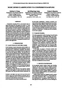
The Focus (FP.F) describes the distribution of the energy in the FP. In particular, FP.F is low if the energy is focused in small regions of the FP, and high if the energy is spread out over the whole FP. The FP.F is computed as mean value of all values in the FP matrix, after normalizing the FP such that the maximum value equals 1. The distance between two pieces of music is computed as the absolute difference between their FP.F values. Figure 2 shows five example histograms of the values in the FPs and the mean thereof (as vertical line). Black Jesus by Everlast (belonging to the genre alternative) has the highest FP.F value (0.42). The song has a strong focus on guitar chords and vocals, while the drums are hardly noticeable. The song Spider by Flex (belonging to eurodance) has the lowest FP.F value (0.16). Most of the songs energy is in the strong periodic beats. Figure 3 shows the distribution of FP.F over different genres. The values have a large deviation and the overlap between quite different genres is significant. Electronic has the lowest values while punk/metal has the highest. The amount of overlap is an important factor for the quality of the descriptor. As we will see later, in the optimal
FP.G
0.1 0.2 0.3 0.4 0.5 −10
−5
0
(a) DB-MS FP.F
FP.G
Punk Jazz Guitar Jazz Electronic Death Metal A Cappella
Fluctuation Patterns
Given a 6-second Sonogram we compute the amplitude modulation of the loudness in each of the 20 frequency bands using a FFT. The amplitude modulation coefficients are weighted based on the psychoacoustic model of the fluctuation strength [6]. This modulation has different effects on our hearing sensation depending on the frequency. The sensation of “fluctuation strength” is most intense around 4Hz and gradually decreases up to a modulation frequency of 15Hz. The FPs analyze modulations up to 10Hz. To emphasize certain patterns a gradient filter (over the modulation frequencies) and a Gaussian filter (over the frequency bands and the modulation frequencies) are applied. Finally, for each piece the median from all FPs representing a 6-second sequence is computed. This final FP is a matrix with 20 rows (frequency bands) and 60 columns (modulation frequencies). Two pieces are compared by interpreting their FP matrices as 1200-dimensional vectors and computing the Euclidean distance. An implementation of the FPs is available in the MA Toolbox [17]. Figure 2 shows some examples of FPs. The vertical lines indicate reoccurring periodic beats. The song Spider, by Flex, which is a typical example of the genre eurodance, has the strongest vertical lines. 3.2.3
FP.F World Pop/Rock Metal/Punk Jazz/Blues Electronic Classical
0.1 0.2 0.3 0.4 0.5
−10
−5
0
(b) DB-L
Figure 3: Boxplots showing the distribution of the descriptors per genre on two music collections. A description of the collections can be found in Section 4.1. The boxes have lines at the lower quartile, median, and upper quartile values. The whiskers show the extent of the rest of the data (the maximum length is 1.5 of the inter-quartile range). Data beyond the ends of the whiskers are marked with plus-signs. combination of all similarity sources, FP.F has the smallest contribution. 3.2.4
Gravity
The Gravity (FP.G) describes the center of gravity (CoG) of the FP on the modulation frequency axis. Given 60 modulation frequency-bins (linearly spaced in the range of 0-10Hz) the CoG usually lies between the 20th and the 30th bin, and is computed as P P jj i FPij CoG = P , (1) ij FPij where FP is a 20×60 matrix and i is the index of the frequency band, and j of the modulation frequency. We compute FP.G by subtracting the theoretical mean of the fluctuation model (which is around the 31st band) from the CoG. Low values indicate that the piece might be perceived slow. However, FP.G is not intended to model the perception of tempo. Effects such as vibrato or tremolo are also reflected in the FP. The distance between two pieces of music is computed as the absolute difference between their FP.G values. Figure 2 shows the sum of the values in the FP over the frequency bands (i.e. the sum over the rows in the FP matrix) and the CoGs marked with a vertical line. Spider by Flex has the highest value (-5.0), while the lowest value (-6.4) is computed for Take Five by the Dave Brubeck Quartet and Surfin’ USA by the Beach Boys. Figure 3 shows the distribution of FP.G over different genres. The values have a smaller deviation compared to FP.F and there is less overlap between different genres.
Classical and a capella have the lowest values, while electronic, metal, and punk have the highest values. 3.3
Combination
To combine the distance matrices obtained with the 4 above mentioned approaches we use a linear combination similar to the idea used for the aligned Self-Organizing Maps (SOMs) [20]. Before combining the distances we normalize the four distances such that the standard deviation of all pairwise distances within a music collection each equals 1. In contrast to the aligned-SOMs we do not rely on the user to set the optimum weights for the linear combination, instead we automatically optimize the weights for genre classification.
4
GENRE CLASSIFICATION
We evaluate the genre classification performance on four music collections to find the optimum weights for the combination of the different similarity sources. We use a nearest neighbor classifier and leave-one-out cross validation for the evaluation. The accuracies are computed as ratio of the correctly classified compared to the total number of tracks (without normalizing the accuracies with respect to the different class probabilities). Genre classification is not the best choice to evaluate the performance of a similarity measure. However, unlike listening tests it is very fast and cheap. In contrast to the ISMIR 2004 genre contest we apply an artist filter. In particular, we ensure that all pieces of an artist are either in the training set or test set. Otherwise we would be measuring the artist identification performance, since all pieces of an artist are in the same genre (in all of the collections we use). The resulting performance is significantly worse. For example, on the ISMIR 2004 genre classification training set (using the same algorithm we submitted last year) we get 79% accuracy without artist filter and only 64% with artist filter. The difference is even bigger on a large inhouse collection where (using the same algorithm) we get 71% without artist filter and only 27% with filter. In the results described below we always use an artist filter if not stated otherwise. In the remainder of this section first the four music collections we use are described. Second, results using only one similarity source are presented. Third, pairwise combinations with spectral similarity (AP) are evaluated. Fourth, all four sources are combined. Finally, the performances on all collections is evaluated to avoid overfitting. 4.1
Data
For our experiments we use four music collections with a total of almost 6000 pieces. Details are given in Tables 1 and 2. For the evaluation (especially to avoid overfitting) it is important that the collections are structured differently and have different types of contents. 4.1.1
DB-S
The smallest collection consists of 100 pieces. We have previously used it in [17]. However, we removed all
classes consisting of one artist only. The categories are not strictly genres (e.g. one of them is romantic dinner music). Furthermore, the collection also includes one non-music category, namely speech (German cabaret). This collection has a very good (i.e low) ratio of tracks per artist. However, due to its size the results need to be treated with caution. 4.1.2
DB-L
The second largest collection has mainly been organized according to genre/artist/album. Thus, all pieces from an artist (and album) are assigned to the same genre, which is a questionable but common practice. Only two pieces overlap between DB-L and DB-S, namely Take Five and Blue Rondo by the Dave Brubeck Quartet. The genres are user defined and inconsistent. In particular, there are two different definitions of trance. Furthermore, there are overlaps, for example, jazz and jazz guitar, heavy metal and death metal etc. 4.1.3
DB-MS
This collection is a subset of DB-ML which has been used as training set for the ISMIR 2004 genre classification contest. The music originates from Magnatune3 and is available via creative commons. UPF/MTG arranged with Magnatune a free use for research purposes. Although we have a larger set from the same source we use it to compare our results to those of the ISMIR’04 results. The genre labels are given on the Magnatune website. The collection is very unbalanced. Most pieces belong to the genre classical and a large number of pieces in world sound like classical music. Some of the original Magnatune classes were merged by UPF/MTG due to ambiguities and the small number of tracks in some of the genres. 4.1.4
DB-ML
This is the largest set in our experiments. DB-MS is a subset of this collection. The genres are also very unbalanced. The number of artists is not much higher than in DB-MS. The number of tracks per artist is very high. The genres which were merged for the ISMIR contest are separated. 4.2 Individual Performance The performances using one similarity source are given in Figure 4 in the first (only spectral similarity, AP) and last columns (only the respective similarity source). AP clearly performs best, followed by FP. The performance of FP.F is extremely poor on DB-S while it is equal to FP.G on DB-L. For DB-MS without the artist filter we obtain 79% using only AP (this is the same performance also obtained on the ISMIR’04 genre contest test set, which indicates that there was no overfitting on the data). Using only FP we obtain 66% accuracy which is very close to the 67% Kris West’s submission achieved. The accuracy for FP.F is 30% and 43% for FP.G. Always guessing that a piece is classical gives 44% accuracy. Thus, the performance of FP.F is significantly below the random guessing baseline. 3
http://www.magnatune.com
In-House Small (DB-S) In-House Large (DB-L) Magnatune Small (DB-MS) Magnatune Large (DB-ML)
Genres 16 22 6 10
Artists 66 103 128 147
Tracks 100 2522 729 3248
Artists/Genre Min Max 2 7 3 6 5 40 2 40
Tracks/Genre Min Max 4 8 45 259 26 320 22 1277
Table 1: Statistics of the four collections. DB-S DB-L
DB-MS DB-ML
alternative, blues, classic orchestra, classic piano, dance, eurodance, happy sound, hard pop, hip hop, mystera, pop, punk rock, rock, rock & roll, romantic dinner, talk a cappella, acid jazz, blues, bossa nova, celtic, death metal, DnB, downtempo, electronic, euro-dance, folk-rock, German hip hop, hard core rap, heavy metal/thrash, Italian, jazz, jazz guitar, melodic metal, punk, reggae, trance, trance2 classical, electronic, jazz/blues, metal/punk, pop/rock, world ambient, classical, electronic, jazz, metal, new age, pop, punk, rock, world
Table 2: List of genres for each collection.
FP 29 30 32 33 30 27 26 25 23 18 17 FP.F 29 28 28 25 20 19 17 17 14
6
1
FP.G 29 31 35 36 37 35 31 29 25 21 15 0
10 20 30 40 50 60 70 80 90 100
(a) DB-S FP 27 30 30 29 30 30 29 28 26 25 23 FP.F 27 27 27 25 24 23 23 22 20 18
8
FP.G 27 30 29 28 27 26 26 25 24 22
8
0
10 20 30 40 50 60 70 80 90 100
(b) DB-L FP 64 63 64 65 65 65 63 63 62 61 58 FP.F 64 66 64 63 63 61 59 58 58 54 28 FP.G 64 64 64 64 63 61 61 61 60 57 42 0
10 20 30 40 50 60 70 80 90 100
(c) DB-MS FP 56 57 57 58 58 57 56 55 55 52 49 FP.F 56 56 56 54 54 53 53 52 52 50 25 FP.G 56 57 56 56 55 54 54 54 53 52 32 0
10 20 30 40 50 60 70 80 90 100
4.4 Combining All Figure 5 shows the accuracies obtained when all similarity sources are combined. There are a total of 270 possible combinations using a step size of 5 percent-points and limiting AP to a mixing coefficient between 100-50% and the other sources to 0-50%. Analogously to the previous results FP.F has the weakest performance and the improvements for the Magnatune collection are not very exciting. As in Figure 4 the smooth changes of the accuracy with respect to the mixing coefficient are an indicator for the robustness of the approach (within each collection). Without the artist filter the combinations on the DB-MS reach a maximum of 81% (compared to 79% using only AP). It is clearly noticeable that the results on the collections are quite different. For example, for DB-S using as little AP as possible (highest values around 45-50%) and a lot of FP.G (highest values around 25-40%) gives best results. On the other hand, for the DB-MS collection the best results are obtained using 90% AP and only 5% FP.G. These deviations indicate overfitting, thus we analyze the performances across collections in the next section.
(d) DB-ML
4.5 Overall Performance Figure 4: Results for combining AP with one of the other sources. All values are given in percent. The values on the x-axis are the mixing coefficients. For example, the fourth column in the second row is the accuracy for combining 70% AP with 30% of FP.F. 4.3
Combining Two
The results for combining AP with one of the other sources are given in Figure 4. The main findings are that combining AP with FP or FP.G performs better than combining AP with FP.F (except for 10% FP.F and 90% AP in DB-MS). For all collections a combination can be found which improves the performance. However, the improvements on the Magnatune collection are marginal. The smooth changes of the accuracy with respect to the mixing coefficient are an indicator that the the approach is relatively robust (within each collection).
To study overfitting we compute the relative performance gain compared to the AP baseline (i.e. using only AP). We compute the score (which we want to maximize) as the average of these gains over the four collections. The results are given in Table 3. The worst combination (using 50% AP and 50% FP.F) yields a score of 0.85. (That is, in average, the accuracy using this combination is 15% lower compared to using 100% AP.) There are a total of 247 combinations which perform better than the AP baseline. Almost all of the 22 combinations that fall below AP have a large contribution of FP.F. The best score is 14% above the baseline. The ranges of the top 10 ranked combinations are 55-75% AP, 5-20% FP, 5-10% FP.F, 10-30% FP.G. Without artist filter, for DB-MS the top three ranked combinations from Table 3 have the accuracies 1: 79%, 2: 78%, 3: 79% (the AP baseline is 79%, the best possible combination yields 81%). For the DB-S collection with-
Rank 1 2 3 4 5 6 7 8 9 10 248 270
AP 65 65 70 55 60 60 75 75 65 55 100 50
Weights FP FP.F 15 5 10 10 10 5 20 5 15 10 15 5 10 5 5 5 10 5 5 10 0 0 0 50
FP.G 15 15 15 20 15 20 10 15 20 30 0 0
DB-S 38 38 38 39 38 39 37 38 38 41 29 19
Classification Accuracy DB-L DB-MS DB-ML 32 67 58 31 67 57 31 67 58 31 65 57 31 66 57 31 66 57 31 67 58 31 66 58 30 66 58 29 65 56 27 64 56 23 61 53
Score 1.14 1.14 1.14 1.14 1.14 1.13 1.13 1.13 1.13 1.13 1.00 0.85
Table 3: Overall performance on all collections. The displayed values in columns 2-4 are the mixing coefficients in percent. The values in columns 5-8 are the rounded accuracies in percent.
100 95 90 85 80 75 70 65 60 55 50 AP 29 30 33 34 39 38 38 39 39 41 41 FP 41 41 38 39 39 36 35 35 32 31 27 FP.F 39 39 41 41 41 38 36 35 29 21 19
Average
1.2 1 0.8
DB−S
1.4
FP.G 35 36 37 39 40 41 41 41 41 37 35 0
5
10 15 20 25 30 35 40 45 50
1 0.6
(a) DB-S
DB−L
1.3 100 95 90 85 80 75 70 65 60 55 50 AP 27 30 31 32 32 32 32 32 31 32 31
1 0.7
FP 30 32 32 32 32 31 31 32 31 31 30 FP.F 31 32 32 32 31 31 30 29 28 26 23 FP.G 32 32 32 32 31 30 29 29 29 28 26 0
5
10 15 20 25 30 35 40 45 50
(b) DB-L 100 95 90 85 80 75 70 65 60 55 50 AP 64 67 68 67 67 67 67 67 67 67 67
DB−MS
1.1 1 0.9
DB−ML
1.1 1 0.9 50
100
150
200
250
FP 68 67 67 67 67 67 66 67 67 65 65 FP.F 66 68 67 67 66 66 65 65 64 64 61 FP.G 67 68 67 67 67 66 65 65 65 64 61 0
5
10 15 20 25 30 35 40 45 50
(c) DB-MS 100 95 90 85 80 75 70 65 60 55 50 AP 56 57 57 58 58 58 58 58 58 58 57 FP 57 58 58 58 58 58 58 58 58 57 57 FP.F 58 58 58 58 57 57 56 56 55 55 53 FP.G 58 58 58 58 58 57 57 57 56 56 54 0
5
Figure 6: Individual relative performance ranked (x-axis) by score (y-axis).
10 15 20 25 30 35 40 45 50
(d) DB-ML
Figure 5: Results for combining all similarity sources. A total of 270 combinations are summarized in each table. All values are given in percent. The mixing coefficients for AP (the first row) are given above the table, for all other rows below. For each entry in the table of all possible combinations the highest accuracy is given. For example, the second row, third column depicts the highest accuracy obtained from all possible combinations with 10% FP. The not specified 90% can have any combination of mixing coefficients, e.g. 90% AP, or 80% AP and 10% FP.G etc.
out artist filter the AP baseline is 52% and the top three ranked combinations have the accuracies 1: 63%, 2: 61%, 3: 62% (the best possible score achieved through combination is 64%). This is another indication that genre classification and artist identification are not the same type of problem. Thus, it is necessary to ensure that all pieces from an artist (if all pieces from an artist belong to the same genre) are either in the training or test set. Figure 6 shows the relative performance of all combinations ranked by their score. As can be seen there are significant deviations. In several cases a combination performs well on one collection and performs poor on another. This indicates that there is a large potential for overfitting if the necessary precautions are not taken (such as using several different music collections). However, another observation is that although there is a high variance the performance stays above the baseline for most of the combinations and there is a common trend. Truly reliable results would require further testing on additional collections.
5 CONCLUSIONS We have presented an approach to improve audio-based music similarity and genre classification. We have combined spectral similarity with three additional information sources based on Fluctuation Patterns. In particular, we have presented two new descriptors and a series of experiments evaluating the combinations. Although we obtained an average performance increase of 14%, our findings confirm the glass ceiling observed in [2]. Preliminary results with a larger number of descriptors indicate that the performance per collection can only be further improved by up to 1-2 percent-points. However, the danger of overfitting is eminent. Our results show that there is a significant difference in the overall performance if pieces from the same artist are in the test and training set. We believe this shows the necessity to use an artist filter to evaluate genre classification performances (if all pieces from an artist are assigned to the same genre). Furthermore, the deviations between the collections suggest that it is necessary to use different collections to avoid overfitting. One possible future direction is to focus on developing similarity measures for specific music collections (analogously to developing specialized classifiers able to distinguish only two genres). However, combining audio-based approaches with information from different sources (such as the web), or modeling the cognitive process of music listening are more likely to help us get beyond the glass ceiling.
ACKNOWLEDGEMENTS This research was supported by the EU project SIMAC (FP6-507142). The Austrian Research Institute for Artificial Intelligence is supported by the Austrian Federal Ministry for Education, Science, and Culture and by the Austrian Federal Ministry for Transport, Innovation, and Technology.
References [1] J.-J. Aucouturier and F. Pachet. Music similarity measures: What’s the use? In Proc ISMIR, 2002. [2] J.-J. Aucouturier and F. Pachet. Improving timbre similarity: How high is the sky? Journal of Negative Results in Speech and Audio Sciences, 1(1), 2004. [3] S. Baumann and O. Hummel. Using cultural metadata for artist recommendation. In Proc WedelMusic Conf, 2003. [4] A. Berenzweig, D. P.W. Ellis, and S. Lawrence. Anchor space for classification and similarity measurement of music. In Proc IEEE Intl Conf on Multimedia and Expo, 2003. [5] A. Berenzweig, B. Logan, D. P. W. Ellis, and B. Whitman. A large-scale evaluation of acoustic and subjective music similarity measures. In Proc ISMIR, 2003. [6] H. Fastl. Fluctuation strength and temporal masking patterns of amplitude-modulated broad-band noise. Hearing Research, 8:59–69, 1982.
[7] J. Foote. Content-based retrieval of music and audio. In Multimedia Storage and Archiving Systems II, 1997. [8] P. Knees, E. Pampalk, and G. Widmer. Artist classification with web-based data. In Proc ISMIR, 2004. [9] B. Logan. Music recommendation from song sets. In Proc ISMIR, 2004. [10] B. Logan and A. Salomon. A music similarity function based on signal analysis. In Proc IEEE Intl Conf on Multimedia and Expo, 2001. [11] B. Logan. Content-based playlist generation: Exploratory experiments. In Proc ISMIR, 2002. [12] B. Logan, A. Kositsky, and P. Moreno. Semantic analysis of song lyrics. In Proc IEEE Intl Conf on Multimedia and Expo 2004, 2004. [13] M. F. McKinney and J. Breebaart. Features for audio and music classification. In Proc ISMIR, 2003. [14] F. Pachet, G. Westerman, and D Laigre. Musical data mining for electronic music distribution. In Proc WedelMusic Conf, 2001. [15] F. Pachet and D. Cazaly. A taxonomy of musical genres. In Proc RIAO 2000 Content-Based Multimedia Information Access, 2000. [16] E. Pampalk. Islands of music: Analysis, organization, and visualization of music archives. MSc thesis, Vienna University of Technology, 2001. [17] E. Pampalk. A Matlab toolbox to compute music similarity from audio. In Proc ISMIR, 2004. [18] E. Pampalk, A. Rauber, and D. Merkl. Contentbased organization and visualization of music archives. In Proc ACM Multimedia, 2002. [19] E. Pampalk, S. Dixon, and G. Widmer. On the evaluation of perceptual similarity measures for music. In Proc Intl Conf on Digital Audio Effects, 2003. [20] E. Pampalk, W. Goebl, and G. Widmer. Visualizing changes in the structure of data for exploratory feature selection. In Proc ACM SIGKDD Intl Conf on Knowledge Discovery and Data Mining, 2003. [21] T. Pohle. Extraction of audio descriptors and their evaluation in music classification tasks. MSc thesis, ¨ TU Kaiserslautern, OFAI, DFKI, 2005. [22] Y. Rubner, C. Tomasi, and L. J. Guibas. The earth movers distance as a metric for image retrieval. Intl Journal of Computer Vision, 40(2), 2000. [23] G. Tzanetakis, G. Essl, and P. Cook. Automatic musical genre classification of audio signals. In Proc ISMIR, 2001. [24] K. West and S. Cox. Features and classifiers for the automatic classification of musical audio signals. In Proc ISMIR, 2004. [25] B. Whitman and S. Lawrence. Inferring descriptions and similarity for music from community metadata. In Proc Intl Computer Music Conf, 2002. [26] A. Zils and F. Pachet. Automatic Extraction Of Music Descriptors From Acoustic Signals. In Proc ISMIR, 2004. [27] E. Zwicker and H. Fastl. Psychoacoustics, Facts and Models. Springer, 1999.