Improving Arterial Performance Measurement Using ... - CiteSeerX

Presentation for ITE District 6 Annual Meeting, July 2007, Portland

1

Improving Arterial Performance Measurement Using Traffic Signal System Data Michael Wolfe, Christopher Monsere, Peter Koonce and Robert L. Bertini, Portland State University

ABSTRACT The characterization of the performance of freeways in real time and on a historical basis has been successfully achieved for many years. The ability to characterize arterial performance has been more elusive. Currently numerous applications of traffic management and traveler information systems include freeways but lack the ability to extend their operation to major arterials. This paper describes methods for quantifying arterial performance using data from signal system loop detectors. Included in the array of metrics are traffic density, total delay, predicted travel time, and signal coordination effectiveness. Methods for determining performance in these areas are adapted for use in quantitatively evaluating arterials in real-time. To assess them, methods are employed to analyze archived data for a segment of Barbur Blvd. in Portland, Oregon. Suggestions for future research are also included. INTRODUCTION Currently, many municipalities offer information about current conditions on local freeway facilities via the Internet or some other media. Fig 1 shows an example for the Portland, Oregon metropolitan area. However, as important as freeways may be for many travelers, it is clearly desirable to collect and disseminate traveler information about arterials. As shown in Fig 1, the major arterials (and some uninstrumented freeway sections) in the region are shown as grey lines due to the absence of data. Travelers would benefit by gaining information about the current traffic conditions on all routes so that potential alternate routes (particularly for short trips) could be evaluated. If performance of arterials were measured over time, transportation managers and operators Fig 1 Portland freeway condition map. would better be able to evaluate the effectiveness of signal timing plans and other operational improvements. In the long run, planning agencies would be able to better monitor the arterial network and understand

Presentation for ITE District 6 Annual Meeting, July 2007, Portland

2

the effects of changing land uses. Similar applications of archived freeway performance have been demonstrated [1]. The objective of this paper is to investigate potential methods to generate meaningful real-time information about arterial performance for traveler information. Since many arterials are instrumented with presence detection (usually inductive loop but also microwave radar and video) as part of their traffic signal systems, this paper identifies suitable metrics utilizing data generated by these systems. An example application of one method based on system detector occupancy is presented using a case study on one major arterial in Portland, Oregon. Performance measures will be validated using automatic vehicle location (AVL) data from buses running simultaneously over the same arterial. Finally, the paper will describe some challenges encountered in applying the methodology as well as topics for future research. ARTERIAL PERFORMANCE The metrics for assessing freeway performance are well understood, and data for computing them are readily obtainable from sensors installed in the freeway—some combination of speed, flow, and occupancy, plus incident records will typically provide a complete picture. As described in Hicks and Carter [2], interrupted flow facilities such as arterials are more challenging because they include interactions between flows of vehicles, pedestrians and bicyclists; lane changing and entry and exit via driveways and side streets; and queuing due to periodic flow interruptions controlled by traffic signals. As a result of these features, traffic conditions can vary widely from point to point along an arterial, making it more difficult to measure conditions from discrete detection points. Table 1 summarizes some potentially useful quantities that can be measured on arterials according to a survey conducted by Shaw [3]. The most useful measure to employ depends on the intended audience, the context, and the communications medium. Hallenbeck and Nee [4] found that tools for evaluating signal performance (such as computing delay, platoon ratio, or number of signal failures) are especially valuable to transportation agencies.

TABLE 1 SELECTED ARTERIAL PERFORMANCE MEASURES Metric Measurement Interval Maximum Speed Average Speed per Vehicle Speed Indexa per Person Density per Distance Running Time per Time Travel Time (cycle, 15 min, hour, Travel Time Variance day) Average Delay Maximum Delay Queue Length Platoon Ratio Number of Stops Signal Failure Duration of Congestion per Day Number of Incidents per Day/Peak Period Duration Incidents per Event Nonrecurring Delay a Ratio of average speed to posted speed.

Location

per Lane per Lane Group per Approach per Segment per Facility per Area

However, when disseminating information to the traveling public performance measures that relate to travel time appear most appropriate. For example, when communicating via variable message signs (VMS), the location of incidents or a travel time estimate for the upcoming corridor is the most desirable. When communicating with travelers on the Web or handheld devices, a map with color-coded

Presentation for ITE District 6 Annual Meeting, July 2007, Portland

3

congestion levels, a function that can provide a travel time estimate between userselected points, or closed-circuit television (CCTV) images would be appropriate. There are a number of current applications of using signal system data for real-time arterial performance including the cities of Los Angeles, California; Bellevue, Washington; and London, United Kingdom. Fig 2 shows an example for London that displays the current conditions from the city’s signal control system. Travel time along an arterial essentially includes two distinct components; the travel time along links between the influence area of traffic signals and the travel time through the signal itself. The traffic flow between signals (nodes) generally behaves like an uninterrupted flow facility and methods to extrapolate Fig 2 London arterial performance map. measured speed at a point (system loop detectors) to estimate link travel time would likely produce results comparable to freeway experience [5]. At the signals themselves, current detection is primarily installed for the purpose of operating the signal and may not be configured to provide data useful for performance estimates. Several authors have proposed methods for estimating travel time that take into account these two components of travel on signalized arterials. Such attempts have either attempted to measure each component directly [6,7,8] or used traffic flow theory to set up relationships between traffic flow and signal control settings [9,10]. Skabardonis and Geroliminis [11] have formulated a model that addresses the problem of collecting data by predicting travel time on a corridor based on count and occupancy data from signal loop detectors, green times, cycle lengths, and offsets for the signals in the corridor. The model is broadly applicable and does not require any location specific calibration. Free-flow travel time is computed, and delay due to various factors is added to that to get predicted travel time. Delay factors include delay incurred by a single vehicle (due to signalization), delay caused by vehicle interactions (due to queues and platoon dispersion), and delay due to signal cycle failure. Because this model outputs travel time and itemized delay, a broad variety of performance measures can be inferred from

Presentation for ITE District 6 Annual Meeting, July 2007, Portland

4

it. These models require cycle-by-cycle data which can be difficult to obtain in real-time for many agencies. This was a limitation for the application proposed here as well. Liang [12] has formulated a method for displaying information about traffic conditions in real-time on the internet. The city of Bellevue, Washington displays a real time map of their downtown area that is color coded, with colors corresponding to the levels of congestion on the corresponding streets. Liang’s model is driven by data collected from existing signal loop detectors. Due to the availability of the data and the suitability of the output for public consumption, it was determined that this model would provide a logical starting point in using the City of Portland’s loop detectors to derive information about arterial performance. The Liang model uses the occupancy data from a system link, and averages it with the link’s previous occupancy level, with a weight determined by a user-defined smoothing constant: On = [Or + On-1 × (S – 1)] / S where On-1 is the previous adjusted occupancy, Or is the most recent reported occupancy, and S is the smoothing constant. The resulting occupancy value is compared to a set of thresholds tailored to the specific intersection. The thresholds correspond to levels of congestion at the intersection, and are configurable in two ways. Liang [12] compared the occupancy data from system detectors (at 300 feet upstream) to that of system detectors for the same intersection and found comparable trends between them. The data taken from system detectors can therefore provide useful information about the state of traffic on the arterial, which is desirable because of the large existing install base of system loop detectors. First, on a system level, it is necessary to specify the number of distinct congestion levels to be distinguished, and the qualitative differences between them. The levels of congestion represent differences perceivable by travelers, particularly if the information is to be displayed as part of a traveler information system. The implementation in Bellevue consists of 4 levels: light, moderate, heavy, and severe. The difference between any two of them is based on the likelihood of signal failure at the intersection— light and moderate congestion levels indicate a high likelihood of getting through the signal in a single cycle, heavy congestion indicates that the traveler will probably need 2 cycles, and at a severe level, traffic is congested enough that a vehicle will usually require 2 or more cycles to clear the intersection. CORRIDOR DESCRIPTION

Presentation for ITE District 6 Annual Meeting, July 2007, Portland

5

The corridor used in this study was Barbur Blvd. (also state route OR-99W) in southwest Portland, Oregon (see Fig 3). The Fig shows the alignment of the study arterial on a map and a schematic representation on the right showing the number of lanes (for the northbound direction) and location of the system detectors used in this analysis. The street names are given for all signalized intersections on the corridor. The study corridor is approximately 5 miles long and had average daily traffic volumes of 25,300 in 2005. The primary flows are northbound in the morning peaks (to downtown Portland) and southbound in the afternoon. A number of circumstances motivated the selection of Barbur Blvd. as the study corridor. First, this arterial is often used as an alternate route for I-5, one of the key commute routes in the Portland area. In fact, the city has installed VMS hardware and developed incident timing plans in conjunction with the Oregon Department of Transportation (ODOT) to utilize northbound Barbur in the event of an incident on I-5. Second, Barbur is one of the better instrumented arterials in the region, with system detector infrastructure in place, and communication capabilities with the central signal system. Finally, the region’s public transit agency, TriMet, runs frequent service and express buses on Barbur the length of the corridor. These buses are equipped with automatic vehicle location (AVL) technology and were exploited as probe vehicles to validate the performance metrics developed in this study. The data gathered from the instrumented arterial and the TriMet buses are described in the following section. DATA In order to gather the data necessary to apply the Liang method to the Barbur Blvd. arterial, the system detectors shown in Fig 3 were configured as count stations in the City’s central signal system. These system detectors are in advance of the signal, ranging from 100 feet to 780 feet upstream from the stop bar. Each count station recorded average values for its constituent detectors, as well as data for the detector that saw the most activity for a given 5 minute period (the “critical” detector as estimated by the TransCore central software). The arterial signal system detector data was collected for a one week Fig 3. Map and schematic of Barbur Blvd. period from Feb 12 through Feb 20, 2007. Critical lane, critical volume, critical occupancy, critical stops, critical speed, total volume, average occupancy, total stops, and average speed were collected for each 5 minute period over the 7 day

Presentation for ITE District 6 Annual Meeting, July 2007, Portland

sample. While the system is capable of collecting finer resolution data (i.e. at the cycle level), the current software is not configured to allow resolution lower than 5 minute aggregation. A software modification to this limitation is currently being explored by the vendor.

6

Sheridan Hooker

Hamilton

Bertha (E) Bertha (W)

The local transit agency (TriMet) has automatic vehicle location (AVL) equipment installed on all of its buses and has an extensive Park & Ride bus dispatch system (BDS) which 2:00 6:00 10:00 14:00 18:00 22:00 collects performance metrics Time (Hours) about each vehicle’s daily activities. At each bus stop (whether the vehicle stops or not) or when a bus opens its doors, the BDS records 26 data elements. These data have been shown to be capable of generating bus vehicle trajectories that are comparable to passenger vehicle trajectories in certain situations [13]. In this research, bus vehicle trajectories were created by plotting the location of the bus at consecutive time points (on average, less than .25 miles apart). The TriMet stop-level AVL data was also collected for the same days as the signal system data. The ability to obtain archived stop-level AVL data for the days and times that the signal detector data was studied has facilitated a unique opportunity to calibrate the arterial performance model. ARTERIAL PERFORMANCE ANALYSIS The objective of the analysis was to demonstrate that the Liang method could be used to generate real-time arterial performance measures for Barbur Blvd. using the available data. As mentioned, the final objective would be communication of current arterial condition to the traveling public via an ATMS such as the one shown in Fig 2. One of the difficulties in employing Liang’s method is the necessity of calibrating the occupancy values to correspond with a measure of congestion that can be communicated to the public. The expectation is that this would be done with a simple color scale. Liang [12] states that several factors should be considered, including the number of lanes in the approach, distance between intersections, free-flow speed, upstream detector distance, signal cycle length, and signal offset. As described, these qualitative calibrations require site-specific knowledge and trial-and-error. This analysis explores some quantitative measures to this calibration process. A number of exploratory plots were generated to validate the data and investigate thresholds for occupancy values. Fig 4 shows a t-x plane for one complete day (Thursday, Feb 16) with the hour of day on the x-axis and distance on the y-axis. The

Presentation for ITE District 6 Annual Meeting, July 2007, Portland

7

measured average occupancy values (in %) expressed as a color with darker colors indicating higher occupancy. The locations of the signalized intersections with system detectors are shown on the y-axis. Travel direction is from the bottom of the figure towards the top. For this typical day, Fig 4 shows the expected congestion pattern. Starting at approximately 7:00AM and lasting until 9:00AM, higher occupancy values are shown from the Bertha (East) detector downstream towards Hamilton and Hooker and detectors, with the highest values at the downstream intersections. This pattern shows the morning peak-hour congestion and is entirely consistent with experience. Because the morning peak hour is the period of greatest activity for this site, further analysis was focused during this time period for the northbound direction. In the plot shown in Fig Speed 4, the intersection at 80 70 Occupancy Hamilton clearly 70 60 experiences the most 60 congestion in the 50 50 morning peak hour. Fig 40 40 5 is a scatterplot that 30 30 shows the 5 minute 20 20 average speeds for a 24 10 10 hour period on Monday, Feb 12 plotted on the 0 0 0:00 3:00 6:00 9:00 12:00 15:00 18:00 21:00 0:00 left y-axis and Time occupancy plotted on Fig 5. Measured speeds and occupancy at Barbur Blvd. and Hamilton, northbound, 2/12/07. the right y-axis. In Fig 5, it is interesting to note that there is very little speed reading between 1:00 AM and 4:30 AM (due to an absence of traffic), a wide variation in readings between 7:00 PM and 12:00 AM, and the relative smoothness of the average speeds in the morning peak period. It appears that throughout much of the day, the distribution of individual preferences for speed throughout the driver population governs what is observed. 80

Occupancy (%)

Speed (mph)

90

In the morning peak period, however, it can be seen that as average occupancy climbs, the average speed decreases to a low value of 3 mph at 7:50AM (occupancy 67.8%). Occupancy peaks 10 minutes later at 8:00AM with a value of 74.6%. The data conform to accepted principles of traffic flow and it is clear that there is a relationship between measured occupancy and the speed, which travelers most readily associate with congestion. Fig 6 displays the flow-density relationship at the intersection of Barbur and Hamilton for the week under study. Barbur Blvd. has three lanes in the northbound direction at this point. Assuming an ideal saturation flow rate of 1,900 vehicles per hour, the maximum

Presentation for ITE District 6 Annual Meeting, July 2007, Portland

8

Flow (veh/hour)

flow rate at this location 4,000 should be around 5,700 3,500 vehicles per hour. 3,000 However, because of the 2,500 presence of the downstream signal, and 2,000 aggregation of the data in 5 1,500 minute bins, the maximum 1,000 observed flow rate is 500 metered by the signal’s effective green to cycle 0 0 10 20 30 40 50 60 70 80 length ratio for the Occupancy (%) northbound direction. The point where observed Fig 6. Flow-occupancy relation at Barbur Blvd. and Hamilton, northbound 2/12/07 -2/20/07. hourly flow levels off with increased occupancy represents the point where the downstream signal starts limiting flow. It is also likely that cycle failures may be occurring during this time period, as occupancy values increase until a recovery begins (in Fig 4). By observation of the figure, the occupancy where these events (speed drop in Fig 4 and flow cutoff) occur in both Figs is around 22%. Using this information, the Liang method was applied and the occupancy was calibrated to show “congestion” where values were greater that 20%. In the example of the condition map shown in Fig 7, a green-yellow-red-black color scheme is used. The threshold between yellow and red was set at 20% occupancy on the contour plots in this paper. Thus, plotting the flow-density relationship at an intersection is a useful tool in determining where the contour thresholds should be set. Another issue encountered in setting up any kind of system for generating arterial performance information is the issue of data resolution. In this study, the distance between detectors ranged from 0.2 to 1.75 mi. The impact of detector spacing on the reliability of travel time predictions at the upper end of that range is substantial. It is therefore important to look at what parts of the arterial a detector can describe with confidence.

N

6:00

8:00

10:00

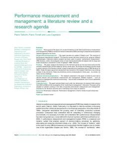
Time (Hours) Fig 7. Time-space contour plot of occupancy for Barbur Blvd., northbound with estimated bus trajectories shown. This plot was generated assuming detector measurement applies downstream to next detector location.

Presentation for ITE District 6 Annual Meeting, July 2007, Portland

9

Fig 7 shows a contour plot for northbound Barbur Blvd. on Feb 12, displaying conditions in the study area for the morning peak according to the initial color thresholds calibrated from the above analysis. The traces overlaid on the plot are the trajectories of buses as they traveled on Barbur Blvd. during this period. To generate this plot, it was assumed that 6:00 8:00 10:00 conditions at a detector Time (Hours) represented conditions from the Fig 8. Time-space contour plot of occupancy for Barbur Blvd., northbound with location of the detector estimated bus trajectories shown. This plot was generated assuming detector measurement applies one-half the distance downstream and upstream to next downstream to the next detector. detector location. Note the bus trajectories at Hamilton around 8:00 AM—the buses slowed down before the black region, but have a fairly steep trajectory (indicating high speed) through the point of highest congestion. This implies this simplifying assumption could be improved. N

Fig 8 shows a contour plot for the same period on Barbur Blvd., for the same length of time. For this plot, it was assumed that the conditions at a detector could be extrapolated upstream to a point halfway to the previous detector, and downstream to a point halfway to the next detector. In this way, the distance from the detector to any point in the traffic stream that the detector described would be minimized. Again, the trajectories of the bus runs have been overlaid onto the contour plot. In this figure, the slowest parts of the buses’ trips correspond much better to the points of highest congestion. CONCLUSIONS The use of system signal loop detector data for assessing arterial performance holds promise. However, further research is necessary to determine the suitable distance from the stop bar and whether the results are related to cycle length and congestion. The data generated by detectors installed for the more specific task of signal control contains a great deal of useful information about local traffic conditions. With care, this information can be extracted and formatted for consumption by the general public. The Liang model offers a rapidly deployable, simple method for displaying information about congestion on arterials. The Skabardonis model is a more complicated, processorintensive method that is more generally applicable and which yields a broader spectrum of information about local conditions. Finally, data from system detectors can be used effectively to quickly and easily assess the effectiveness of signal coordination.

Presentation for ITE District 6 Annual Meeting, July 2007, Portland

10

For successful application, data should be collected frequently (at least once per cycle), and data should be transmitted from the signal to the operations center on a basis that is as close to real time as possible. The lack of this capability seriously degrades the ability to use detector data to extract useful information, if not making it completely impossible, whereas improving polling frequency makes use of this data for ITS applications more robust. The current generation of signal control hardware is generally incapable of this level of performance and communication, unfortunately, and is thus a barrier to broader implementation and use of available data and information. However, newer installations of signal systems have potential to allow detailed real-time measurement with increased communication and detection capability. ACKNOWLEDGEMENT Funding and support for this project is provided by the National Science Foundation, Oregon Department of Transportation., Federal Highway Administration, City of Portland, and TriMet. The authors particularly thank Bill Kloos and Willie Rotich of the City of Portland and David Crout of TriMet. Matthew Berkow also assisted with the AVL data. REFERENCES [1] R. L. Bertini, S. Hansen, S., A. Byrd, and T. Yin. “PORTAL: Experience Implementing the ITS Archived Data User Service in Portland, Oregon.” Transportation Research Record: Journal of the Transportation Research Board, No. 1917, Transportation Research Board of the National Academies, Washington, D.C., 2005, pp. 90-99. [2] B. Hicks, and M. Carter. What Have We Learned About Intelligent Transportation Systems? Chapter 3. U.S. Department of Transportation, Washington, D.C. 2000. [3] T. Shaw, NCHRP Synthesis 311 --Performance Measures of Operational Effectiveness for Highway Segments and Systems. Transportation Research Board, Washington, D.C. 2003. [4] J. Nee and M. Hallenbeck. Surveillance Options For Monitoring Arterial Traffic Conditions. Research Project T1803, Task 14. Washington State Transportation Center (TRAC), 2001. [5] C. Monsere, C., A. Breakstone, R.L. Bertini, R.L., D. Deeter, G. McGill. “Validating Dynamic Message Sign Freeway Travel Time Messages Using Ground Truth Geospatial Data.” Transportation Research Record: Journal of the Transportation Research Board No. 1959, Transportation Research Board of the National Academies, Washington, D.C., 2006, pp. 19-27. [6] J.Y.K Luk,. and L.W. Cahill. “On-Line Estimation of Platoon Delay.” Australian Road Research Board, Proceedings 13th Annual Conference, Part 7 – Traffic, 13, pp. 133-148. 1986 [7] B. Hellinga, and R. Gudapati.. “Estimating Link Travel Times for Advanced Traveler Information Systems.” Proceedings of the Canadian Society of Civil Engineers, 3rd Transportation Speciality Conference. London, Ontario. 2000. [8] H.M. Zhang. “Link-Journey-Speed Model for Arterial Traffic.” Transportation Research Record 1676. pp. 109-115. Transportation Research Board, Washington, D.C. 1999.

Presentation for ITE District 6 Annual Meeting, July 2007, Portland

11

[9] A.P.Tarko, G. Rajaraman, and D. Boyce. Travel Time Prediction in Intelligent Transportation Systems. NCHRP ITS-IDEA Program. Project ITS-49. Purdue Research Foundation, Purdue University, West Lafayette, Indiana. 1997 [10] L. Fu, B. Hellinga, and Y. Zhu. “An Adaptive Model for Real-Time Estimation of Overflow Queues on Congested Arterials.” Proceedings of 2001 IEEE Intelligent Transportation Systems Conference. Oakland, California. 2001. [11] A. Skabardonis and N. Geroliminis. Real-Time Estimation of Travel Times On Signalized Arterials. Presented at 16th International Symposium on Transportation and Traffic Theory, University of Maryland, July 2005. [12] F. Liang. Development of the Bellevue Real Time Arterial Traffic Flow Map. 2006 ITE District 6 Annual Meeting, Honolulu, Hawaii, 2006. [13] Bertini, R.L. and Tantiyanugulchai, S. “Transit Buses as Traffic Probes: Empirical Evaluation Using Geo-Location Data.” Transportation Research Record: Journal of the Transportation Research Board, No. 1870, Transportation Research Board of the National Academies, Washington, D.C., 2004, pp. 35-45.