Improving Bag-of-Words Model with Spatial Information Edmond Zhang, Michael Mayo The University of Waikato, Knighton Road, Hamilton, New Zealand. Email:
[email protected]
Abstract Bag-of-Words (BOW) models have recently become popular for the task of object recognition, owing to their good performance and simplicity. Much work has been proposed over the years to improve the BOW model, where the Spatial Pyramid Matching technique is the most notable. In this work, we propose three novel techniques to capture more refined spatial information between image features than that provided by the Spatial Pyramids. Our techniques demonstrate a performance gain over the Spatial Pyramid representation of the BOW model. Keywords: Bags-of-words, SIFT Keypoints, Spatial Pyramid Matching, Object Recognition
0
1
Introduction
This paper addresses the problem of object categorization from images. The task is one of the most challenging problems in computer vision, especially when images contain occlusion and background clutter. Appearances of objects belonging to the same category may vary significantly due to changes in viewpoint, scale and deformation. Recently, appearance-based methods [1][2][3] have been successfully applied to the problem of generic object class categorization. A popular strategy is the Bag-of-Words (BOW) model [1], which represents an image as an orderless collection of local features and has shown impressive levels of performance [4][5][6], in spite of the simplicity of the scheme. The BOW model, however, discards the spatial relationships of local descriptors, which severely limits its descriptive power. One of the most successful solutions to this problem, described in the seminal work by Lazebnik et al. [7], is called Spatial Pyramid Matching (SPM). Spatial relationships between image features are important in the sense that they provide a kind of ‘linkage’ information between independent image features. We believe that this information will help us better understand how object parts are related to each other, and in theory, enable classifiers to better discriminate object categories from each other. In this paper, we propose three exten0 978-1-4244-9631-0/10/$26.00
c
2010 IEEE
sions to the SPM model. We argue that objects belonging to the same category exhibit significant regularity in their geometry, and that this information should and can be incorporated into object recognition systems. In this paper, we propose three novel extensions to the SPM approach. More precisely, we introduce three techniques for capturing spatial information based on the BOW model. They are pairs frequency histogram, shapes frequency histogram and the binned log-polar representation of image features. Furthermore, we also experiment with various combinations of spatial and feature frequency information. Since the captured spatial information is based on image labels, they should be complementary to the original frequency histogram of words, as they capture different types of dependencies [8]. The rest of the paper is organized as follows. In Section 2 we will discuss the original concept of the BOW model, followed by a selection of previous works on incorporating spatial information. We then explain our proposed algorithms in Section 3. In Section 4 we will present the datasets and experimental results. Finally, we will conclude this work in Section 5.
2
Previous Work
The BOW model has shown remarkable performance in a wide range of object recognition tasks, in spite of its simplicity. The key idea is that images can be represented by different distributions of visual words (usually SIFT keypoints [9]). A BOW is then built as a histogram over visual
Figure 1: Spatial pyramid matching.
word occurrences. More precisely, building a BOW representation involves the following steps: feature detection, feature description, codebook construction and classification. In its basic form, the BOW method discards all spatial information about how features are related and distributed across images. Over the years, many works have been proposed to improve the original BOW model, such as generative methods [10][11] for modelling the co-occurrence of image features, and discriminative codebook learning in [12][13][14]. In this paper, we focus on discovering spatial relationships between image features. Sivic et al., in [15] were one of the first in attempt to incorporate topological information by joining features into pairs. Zhang et al., in [5], utilizes proximity between features, measured by distance (normally L2) between feature coordinates. However, these approaches exploits the weakness of the dataset, where the object of interest are almost always located in the middle of images and are roughly aligned. Thureson et al. further extends on the pairs-of-features approach by organizing features into triplets in [16]. Local spatial information is also represented in a template-based model in [17], which introduces the concept of geometric blur. Berg et al. later further extended the geometric blur concept in [18], where second order spatial information is utilized to solve the correspondence between geometric blur features. By discovering pairwise configurations between edges, Leordeanu et al. in [19] have proposed the use of edge fragments for category recognition, where model parameters are learned sequentially. Most recently, the spatial pyramid matching model (SPM) by Lazebnik et al. [7] have demonstrated promising results. Figure 1 illustrates the basic idea behind the SPM model. The SPM model builds on the Pyramid Matching kernel by Grauman and Darrell [4]. Broadly speaking, pyramid matching works by placing a sequence of increasingly coarser grids over the image and taking a weighted sum of the number of matches that occur at each scale. Feature matches from finer scales are given more weight.
It is important to note that matches found in scale L also include all the matches found at the finer scale L - 1. Lazebnik et al. argued that because the pyramid matching kernel is simply a weighted sum of histogram intersections, they implemented K L as a single histogram intersection of long vectors formed by concatenating the weighted histogram of all channels at all resolutions [1]. In that, spatial pyramids repeatedly subdivide an image, computing all features repeatedly for all progressively smaller sub-images. The first image is always the global image, and then the image is divided into 2 × 2 sub-images, and features are computed from each of those. The image may then be further subdivided, this time into 4 × 4 subregions, and so on. For a spatial pyramid with l levels, the maximum granularity will be a division of an image into 2l × 2l−1 sub-images. This means that when L = 0, the feature vector size is the size of the codebook, M .
3
New Methods for Capturing Geometrical Information
In this section we describe methods for exploiting and capturing geometrical information between image features. Because all three of our algorithms are build on the visual words from the BOW model, it is important that we explain how these words are produced in detail. To this end, we will first explain the steps that we took in order to produce the vocabulary, before explaining our proposed algorithms.
3.1
Preprocessing from SIFT Keypoints to Visual Dictionary
Recall that there are two categories of approaches in sampling areas of interest from images – using scale invariant detectors and dense sampling. For this work, we took advantage of the second approach. Our reason for this is twofold. Firstly, scale invariant detectors are not known to be good at capturing uniform information such as sea, sky or flat surfaces – information that is essential for our work. Secondly, research by Fei-Fei et al. [20] found that dense features work better for scene classification and that random sampling of keypoints work nearly as well as keypoints selected by detectors [21]. In order to construct our visual dictionary, we first compute a dense overlapped grid of 16 × 16 pixels over the entire image, with a spacing of 8 pixels per grid. We then use Lowe’s high dimensional SIFT descriptor to describe each of the 16 × 16 patches. Each descriptor consists of 128-dimensions. Kmeans clustering is then utilized to group similar
Figure 4: Discovering pairs of labels. Figure 2: Dense sampling of an image before representing features with image label grid.
image patches (now in SIFT descriptor format) into M bins, where M is the vocabulary size for our experiments and M = 200, 400 or 600. In order to simplify the problem into more intuitive and describable terms, we visualize each descriptor as a label, the label being the bin number that the descriptor most closely matches in L2 distance. For example, if a patch descriptor most closely matches cluster centre 202, then that patch is replaced with 202. Figure 2 is an example of this representation. This is the image representation used by all three of our following approaches.
3.2
Approach 1: Pairs Frequency Histogram
Our first model is inspired by the success of the vector-space model for text document representation. After the image is represented by a simple vocabulary of labels of size M (see Figure 2), it is possible to apply many successful text mining techniques such as tf-idf weighting, stop word removal and feature selection [22]. This representation is analogous to the document representation in terms of form and semantics. That is, words convey meaning of the document just as visual words carry visual characteristics of the image. We propose to discover pairs of frequent labels. Unlike [10], our model works by looking for matching labels within a predefined area. We do this by first computing predefined grids (overalpped) over the entire image label grid, where the grid size used is 3 × 3. Figure 3 demonstrates how this grid is formed. For each of the grids, we use the middle label as the reference label to compare its neighbouring labels for matches. We decided to look for pairs of the same label only, because it is simply not feasible to include all possible label combinations. For example, if M = 200, then the number of possible combinations of all 200 labels is a 200 ×
200 = 40000. However, once SPM is applied, the the size of the feature vector will quickly jump to 21 × 40000 = 840000 dimensions when L = 2. Once all pairs are accounted for, we then build a frequency histogram on the number of pairs, where the size of the feature vector is the same as M . See Figure 4 for example on how pairs of labels are discovered.
3.3
Approach 2:Shapes Frequency Histogram
Our second model focuses on capturing the shapes of image features, based on the Local Binary Patterns (LBP) [23]. Although originally used in the domain of texture recognition, this feature type has also recently been found to be effective for generic image recognition. Briefly, in its original form (but not in our approach), a LBP is a property of a pixel. The pixels in circular neighbours at distance r are examined (bilinear interpolation being used if necessary), and a binary string of length n is constructed such that the it h bit of the string is 1 if the neighbours intensity exceeds that of the pixel, and 0 otherwise. Neighbours must be equally spaced around the perimeter of the circle. If, upon a circular transversal of the bit-string, there are two or less 0 to 1 or 1 to 0 transitions, then the LBP is considered uniform and assigned to a category specified by the number of 1s in the string. LBPs tend to capture the edges, curves, peaks and troughs in an image. In this approach, it is the LBP shapes formed by the labels and not the pixels that we are most interested in. We modify the standard LBP approach to treat neighbouring labels as pixels, as well as converting the 8 bit binary string into a decimal number. For example, 00000011 = 3. This enables us to assign all possible shapes to 256 different bins, which can then be turned into a frequency histogram when this is applied to the entire image label grid. Figure 5 depicts an example. One advantage of this approach is that we are not limited to shapes formed by any particular fea-
Figure 3: A set of overlapped, predefined grids over entire image.
Figure 5: proach.
Representing shapes with LBP-like ap-
tures, instead, because we use the middle label as the reference label to compare its neighbouring labels, this enables the capturing of shapes formed by any labels. In addition, recall that with the original LBP approach, if the neighbour’s intensity exceeds that of the middle pixel, 1 will be assigned to the neighbour, and 0 otherwise. We did not adopt this approach because even though labels are represented by a number, they are not related in any form. For example, in our formulation, label 100 is not greater than label 2, as the labels represent different type of features rather than pixel intensities. Instead, we look for labels around the reference label for matches, since only matching labels are related meaningfully.
3.4
Approach 3: Binned Log-Polar Representation
Our last model focuses on mapping the distribution of labels within the image, utilizing a binned log-polar representation. Belongie et al. in [24] first proposed the binned log-polar scheme as a descriptor for the purpose of shape matching. In the original work, a histogram of the distribution of points over relative positions was used as a compact, yet highly discriminative descriptor. In order to make the descriptor more sensitive to positions of nearby sample points than to those points far away, bins are uniform in logj polar space, where sample points on a shape can express the configu-
Figure 6: Binned log-polar representation of labels.
ration of the entire shape relative to the reference point. The descriptor can be applied to greyscale images, but it is very dependent on brightness values. Hence it is more applicable for line drawings. For our work, we use the image centre as the reference point of origin and image features (labels) are treated as points. However, unlike the original implementation, we distinguish the type of points, rather than treating them equally. The benefits of this representation are twofold. First, it results in a compact, yet discriminative descriptor for each image feature (label). Second, the representation accounts for increasing positional uncertainty with distance from the point of origin. See Figure 6 for an example of our log-polar representation. After computing the distribution for every label, we simply concatenate all histograms (a histogram per label) to form a large single feature vector, where the size is M × 32.
4
Evaluation
In the first part of this section, we describe the datasets used to evaluate out new algorithms, and then describe the experiments we performed, and give the result.
4.1
Datasets
We evaluate our three proposed models on three popular datasets: Caltech101 [25], Graz02 [26] and
15 Scenes [27]. Figure 7 illustrates some examples of the three datasets. 4.1.1
Caltech101 [25]
This is probably one of the most diverse datasets in the research community. There are in total a 101 object categories in the dataset, where each object class contains between 31 and 800 images. The resolution for most of the images is about 300 by 300 pixels. For this dataset, we follow the experimental setup of Zhang et al. [5]. Specifically, 30 images per class are used for training and up to 25 images are tagged as test images.
worked well across all three datasets. When combined with BOW frequency histogram, we repeatedly achieve performance improvements over the original BOW work. This method is fundamentally the same as the BOW frequency histogram, however, it differs in what it tries to capture. Instead of single features, this method counts the frequency of pairs of features occurring at a close proximity. 4.3.2
Shapes Frequency Histogram
This method did not perform as well as our other two proposed methods, usually underperforms BOW by a few percent. The motivation behind this approach is to capture the ‘shape’ of features, utiliz4.1.2 15 Scenes [26] ing the LBP scheme. The main reason for the poor performance, we argue, is not due to the concept The 15 scenes dataset contains fifteen categories. of capturing shapes, but mainly due to the size Each category contains 200 to 400 images with the of image patches and codebook. The image patch average size about 300 by 250 pixels. For this size is 16 × 16 for this work, which might be too dataset, we followed the experimental setup of Lazeb- large to capture unique image features for the LBP nik et al. [7]. That is, for each of the categories, method to take advantage of. The other issue is 100 images are randomly selected for training and the codebook size. Since M is relatively small, too the remaining images are tagged as test images. many dissimilar image features are being treated as the same, this is a major disadvantage for ‘strict’ 4.1.3 GRAZ-02 [27] edge-capturing methods like LBP. The dataset contains four categories: Bike, Person, 4.3.3 Log-Polar Representation Cars and Background. This dataset is much more complex that the Caltech101 dataset in terms of This method worked well on all of the datasets, intra-class variation, such as illumination, scale, both on its own and combined with the BOW frepose, viewing angle, occlusion, and clutter. We folquency histogram. Table 4 illustrate the recognilow the experimental setup of Opelt [27]. Namely, tion accuracy of using the log-polar representation we took a training set consisting of 150 images of alone. In this implementation, because the centre the object category as positive images and 150 of of the log-polar grid is always located on the middle the counter-class as negative images. The tests of the image, have contributed to the good perforwere carried out on 300 images half belonging to mance of this method for the Caltech101 dataset, the category and half not. where the object of interest are almost always located on the middle of the image. The log-polar 4.2 Methods grid was able to capture the distribution of the features from the centre, evenly. However, because of We report the experiment setup and results in this this, the log-polar approach did not perform as well section. Multi-class classification is done with SVM on the 15 Scenes dataset, where the dataset is not classifier and the SMO learning algorithm, with deabout objects, but about scenes. Unlike objects, it fault parameters as specified in WEKA V.3.5.5 [28]. was difficult to capture meaningful distribution of All experiments are repeated 10 times with differfeatures as there are no specific shapes to a scene. ent randomly selected training and testing splits. Finally, our results were comparable if not better The final result is reported as the means and stanthan the Graz-02 dataset, where the original BOW dard deviation accuracy of the individual runs. We did not perform well. first show experiment results using only the proposed models, then follow this with results from combining our models with the original frequency histogram and SPM.
4.3 4.3.1
Evaluation Pairs Frequency Histogram
For such an elegant and simple attempt at capturing spatial information, the pairs frequency method
5
Discussion and Conclusion
Our goal in this work is to capture geometric information between image features, to improve the bag-of-words model for object recognition. To this end, we have proposed three approaches in achieving this: pairs frequency, shapes frequency and the binned log-polar representation.
Figure 7: The GRAZ-02, 15 Scenes and Caltech101 dataset.
Table 1: Results for Caltech101, our methods combined with original BOW.
Spatial Pyramid Matching (SPM) BOW Baseline Pairs Frequency + BOW, M = 200 Pairs Frequency + BOW, M = 400 Pairs Frequency + BOW, M = 600 Shapes Frequency + BOW, M = 200 Shapes Frequency + BOW, M = 400 Shapes Frequency + BOW, M = 600 Log-Polar + BOW, M = 200 Log-Polar + BOW, M = 400 Log-Polar + BOW, M = 600
L=0 41.2% 41.47% ±1.5 43.7% ±1.8 43.82% ±1.9 43.99% ±1.5 43.4% ±1.4 42.32% ±1.3 63.8% ±0.9 62.6% ±0.9 61.34% ±1.1
L=1 55.9% 55.34% ±1.1 57.83% ±0.9 57.24% ±1.2 54.77% ±1.3 55.43% ±1.1 56.02% ±1.1 65.45% ±0.8 64.32% ±0.8 62.32% ±0.9
L=2 63.6% 62.18% ±0.9 64.95% ±0.8 64.76% ±1.1 61.98% ±0.9 62.22% ±0.9 61.58% ±1.0 65.93% ±1.0 65.24% ±0.9 63.1% ±0.7
Table 2: Results for 15 Scenes, our methods combined with original BOW.
Spatial Pyramid Matching (SPM) BOW Baseline Pairs Frequency + BOW, M = 200 Pairs Frequency + BOW, M = 400 Pairs Frequency + BOW, M = 600 Shapes Frequency + BOW, M = 200 Shapes Frequency + BOW, M = 400 Shapes Frequency + BOW, M = 600 Log-Polar + BOW, M = 200 Log-Polar + BOW, M = 400 Log-Polar + BOW, M = 600
L=0 72.2% 74.3% ±1.4 74.39% ±1.6 73.12% ±1.5 70.9% ±1.9 70.12% ±1.8 69.83% ±1.9 74.89% ±1.7 75.34% ±1.9 75% ±2.0
L=1 77.9% 78.91% ±1.4 79.05% ±1.3 78.98% ±1.4 75.44% ±1.1 76.23% ±1.6 74.34% ±1.8 79.45% ±1.2 79.8% ±1.0 78.56% ±1.5
L=2 79.4% 80.93% ±1.1 81.54% ±1.3 80.56% ±1.1 77.3%±0.9 78.23% ±1.5 77.45%±1.1 81.36% ±0.8 81.5% ±0.7 80.98% ±1.1
Table 3: Results for GRAZ-02 (Bike), our methods combined with original BOW.
Spatial Pyramid Matching (SPM) BOW Baseline Pairs Frequency + BOW, M = 200 Pairs Frequency + BOW, M = 400 Pairs Frequency + BOW, M = 600 Shapes Frequency + BOW, M = 200 Shapes Frequency + BOW, M = 400 Shapes Frequency + BOW, M = 600 Log-Polar + BOW, M = 200 Log-Polar + BOW, M = 400 Log-Polar + BOW, M = 600
L=0 63.45% 65.81% ±2.6 65.12% ±2.4 64.98% ±2.5 63.09% ±2.5 63.11% ±2.3 62.19% ±2.4 64.67% ±2.4 65.34% ±2.2 64.17% ±2.3
L=1 65.13% 69.9% ±2.1 69.1% ±1.9 68.19% ±2.0 64.44% ±2.1 64.5% ±1.9 63.23% ±1.8 66.1% ±1.9 66.13% ±1.8 65.92% ±2.0
L=2 66.34% 70.11% ±1.8 71.49% ±1.6 70.1% ±1.7 65.92% ±1.9 65.11% ±1.7 64.12% ±1.6 68.5% ±1.4 68.15% ±1.5 67.12% ±1.3
Table 4: Results for using Log-polar representation alone on the three datasets.
Dataset Caltech101 Graz-02 (Bike only) 15 Scenes
BOW + SPM Baseline 63.6% ±0.9 69.34% ±1.7 79.4% ±0.3
Log-Polar alone 62.67% ±1.5 68.76% ±1.4 74.5% ±0.8
Both the pairs frequency and binned log-polar modis simpler since it works without combining other representations. It is interesting to compare and/or els, when combined with the BOW model, have combine these approaches in the future. outperformed the original BOW method by about 2% to 3% across the three diverse datasets. The In Wang et al. [30], which describes a completely LBP representation of the shapes frequency, howdifferent approach to ours, they represent objects ever, did not perform as well. Perhaps the most using histograms of oriented gradients that incornotable conclusion is the performance of the binned porate detailed spatial distribution of objects colour log-polar representation, which performed well alone across different body parts. However, this method on its own, without combining with the original relies on objects having similar poses and observed BOW frequency histogram and spatial pyramid matchin good quality data. It is evident that under more ing. realistic conditions texture and shape information are either non-existent or unreliable due to low imIn [7], Lazebnik et al. found that their spatial pyraage quality. Moreover, they use low level(oriented mid matching scheme is most effective when M = gradients) whereas we use image features. Thus, 200. They tried different codebook sizes, however, the effectiveness of this method is unclear for the they did not report any performance gains. For real world object categorization problem. our proposed methods, across all three datasets, we constantly found that our methods work best when For future work, we are currently investigating the M = 400. Perhaps the main reason is that if the possibility of extending the promising binned logcodebook size is small, too many unrelated patches polar model, by improving the reference label selecwill be grouped together, and if the codebook size tion and the capability to handle multiple points is large, then similar features will not be seen as of origins. the same. The three proposed approaches, though similar to earlier work by Saverse et al. [29] and Wang et al. [30], are different in many respects. The correlograms approach proposed by Savarese et al. is used to measure the distribution of distances between all pairs of visual labels and then applied to category classification tasks (with combination of label distribution). Interestingly, in their paper, correlograms performs much worse than the standard bags-of-words model. In comparison, our pairs of feature approach captures spatial information between visual words, which is more reliable and sparse. In addition, our method
References [1] G. Csurka, C. R. Dance, L. Fan, J. Willamowski, and C. Bray, “Visual categorization with bags of keypoints,” in ECCV, 2004, pp. 1–22. [2] G. Dorke and C. Schmid, “Object class recognition using discriminative local features,” in IEEE, PAMI, Submitted. [3] C. Schmid, G. Dorko, K. M. S. Lazebnik, and J. Ponce, “Pattern recognition with local invariant features,” in Handbook of Pattern recognition and computer vision, 2005.
[4] K. Grauman and T. Darrell, “Pyramid matching kernel: Discriminative classification with sets of image features,” in ICCV, 2005. [5] J. Zhang, M. Marszalek, S. Lazebnik, and C. Schmid, “Local features and kernels for classification of texture and object categories,” in INRIA, 2005.
[19] M. Leordeanu, M. Hebert, and R. Sukthankar, “Beyond local appearance: Category recognition from pairwise interactions of simple features,” CVPR, 2007. [20] L. Fei-fei., “A bayesian hierarchical model for learning natural scene categories,” in In CVPR, 2005, pp. 524–531.
[6] J. Winn, A. Criminisi, and T. Minka, “Object categorization by learned universal visual dictionary,” in ICCV, 2005.
[21] E. Nowak, F. Jurie, and B. Trigg, “Sampling strategies for baf-of-features image classification,” in ECCV, 2006.
[7] C. Schmid, “Beyond bags of features: Spatial pyramid matching for recognizing natural scene categories,” in CVPR, 2006, pp. 2169– 2178.
[22] Y. Jun, J. Yu-Gang, H. A. G., and N. ChongWah, “Evaluating bag-of-visual-words representations in scene classification,” in MIR ’07. NY, USA: ACM, 2007, pp. 197–206.
[8] J. Wu and J. M. Rehg, “Beyond the euclidean distance: Creating effective visual codebooks using the histogram intersection kernel,” in ICCV, 2009.
[23] T. Menp and M. Pietikinen, “Texture analysis with local binary patterns,” in Handbook of Pattern Recognition and Computer Vision, 2005.
[9] D. Lowe, “Distinctive image features from scale-invariant keypoints,” in IJCV, 2004.
[24] S. Belongie, J. Malik, and J. Puzicha, “Shape matching and object recognition using shape contexts,” PAMI, 2001.
[10] P. Quelhas, F. Monay, J. m. Odobez, D. Gatica-perez, and T. Tuytelaars, “Modeling scenes with local descriptors and latent aspects,” in ICCV, 2005, pp. 883–890. [11] O. Boiman, “In defense of nearest-neighbor based image classification,” in CVPR, 2008. [12] F. Jurie and B. Triggs, “Creating efficient codebooks for visual recognition,” in ICCV. IEEE Computer Society, 2005, pp. 604–610.
[25] L. Fei-fei, “Learning generative visual models from few training examples: an incremental bayesian approach tested on 101 object categories,” in CVPR, 2004. [26] R. Fergus, P. Perona, and A. Zisserman, “Object class recogntion by unsupervised scaleinvariant learning,” in CVPR, 2003, pp. 264– 271.
[13] F. Moosmann, B. Triggs, and F. Jurie, “Fast discriminative visual codebooks using randomized clustering forests,” in NIPS, 2006.
[27] A. Opelt, M. Fussenegger, A. Pinz, and P. Auer., “Weak hypotheses and boosting for generic object detection and recognition,” in ECCV, 2004.
[14] L. Yang, R. Jin, and R. Sukthankar, “Unifying discriminative visual codebook generation with classifier training for object category reorganization, cvpr,” 2008.
[28] I. H. Witten and E. Franks, “Data mining: practical machine learning tools and techniques with java implementations,” 2002.
[15] J. Sivic, B. C. Russell, A. A. Efros, and A. Zisserman, “A bayesian hierarchical model for learning natural scene categories,” in ICCV, 2005.
[29] S. Savarese, J. Winn, and A. Criminisi, “Discriminative object class models of appearance and shape by correlatons,” in In IEEE Computer Vision and Pattern Recognition, 2006, pp. 2033–2040.
[16] J. Thureson and S. Carlsson, “Appearance based qualitative image description for object class recognition,” in ECCV, 2004. [17] A. C. Berg and J. Malik, “Geometric blur for template matching,” in CVPR, 2001. [18] ——, “Shape matching and object recognition using low distortion correspondence,” in CVPR, 2005.
[30] X. Wang, G. Doretto, T. B. Sebastian, J. Rittscher, and P. H. Tu, “Shape and appearance context modeling,” in ICCV, 2007, pp. 1–8.