Improving Bankruptcy Prediction in Micro-Entities by Using Nonlinear ...

JEL classification: C45, G33, G21, D81 Keywords: bankruptcy models, micro-entities, credit risk, non-financial information, artificial neural network, logistic regression

Improving Bankruptcy Prediction in Micro-Entities by Using Nonlinear Effects and Non-Financial Variables Antonio BLANCO-OLIVER—University of Seville, Spain ([email protected]), corresponding author Ana IRIMIA-DIEGUEZ—University of Seville, Spain ([email protected]) María OLIVER-ALFONSO—University of Seville, Spain ([email protected]) Nicholas WILSON—Leeds University Business School, UK ([email protected])

Abstract The use of non-parametric methodologies, the introduction of non-financial variables, and the development of models geared towards the homogeneous characteristics of corporate sub-populations have recently experienced a surge of interest in the bankruptcy literature. However, no research on default prediction has yet focused on micro-entities (MEs), despite such firms’ importance in the global economy. This paper builds the first bankruptcy model especially designed for MEs by using a wide set of accounts from 1999 to 2008 and applying artificial neural networks (ANNs). Our findings show that ANNs outperform the traditional logistic regression (LR) models. In addition, we also report that, thanks to the introduction of non-financial predictors related to age, the delay in filing accounts, legal action by creditors to recover unpaid debts, and the ownership features of the company, the improvement with respect to the use of solely financial information is 3.6%, which is even higher than the improvement that involves the use of the best ANN (2.6%).

1. Introduction In the wake of the financial crisis it is clear that lender risk models and rating systems failed to adequately present the risks in the corporate sector. For this reason, both academics and practitioners are opening new lines of research that strive to improve the performance of existing bankruptcy models. One of the most fruitful lines of research is the development of bankruptcy models specifically designed for each company feature, such as size (e.g. Altman and Sabato, 2007), industry (e.g. Chava and Jarrow, 2004) and age (e.g. Wilson and Altanlar, 2014). Along these lines, Tascon and Castano (2012) suggest that the more homogeneous the characteristics of the companies used for the construction of a prediction model are, the better their predictive capacity will be. In the same line, Internal Ratings Based (IRB) systems, under Basel recommendations, also suggest to the lender to build risk models geared towards the specific characteristics of corporate sub-populations (e.g. large corporations, private companies, listed companies, industry-specific models), tuned to changes in the macro environment and, of course, tailored to the available data. Based on this framework, this paper proposes a bankruptcy model specifically designed for a new, never-before-studied and largely relevant company segment: micro-entities (MEs). Micro-entities have recently been defined by the Competitiveness Council of the European Union as those companies with an annual turnover of less 144

Finance a úvěr-Czech Journal of Economics and Finance, 65, 2015, no. 2

than EUR 700,000, total assets of less than EUR 350,000, and average number of employees during the financial year of no more than ten (Official Journal of the European Union, 2012). Micro-entities (and all small businesses in general) have great quantitative importance since they represent the vast majority of all firms in developed economies and they constitute a segment of firms with homogenous characteristics and problems. The most relevant intrinsic characteristics and problems of MEs are (a) their excessive difficulties when attempting to access bank funding sources (Ciampi and Gordini, 2013) and (b) their limited financial information due to the fact that MEs file abridged accounts (Berger and Frame, 2007). Therefore, we examine a large set of micro-entity data on the presumption that existing parametric bankruptcy models developed for small and medium-sized enterprises (SMEs) might not explain micro-entity defaults with the same statistical effectiveness or efficiency as models estimated using data drawn strictly from the micro-entity population. To build this specific default prediction model for MEs, we also incorporate two other novel trends in this field by (a) introducing non-financial and macroeconomic information as predictor variables (e.g. Grunert et al., 2005; Altman et al., 2010; Moon and Sohn, 2010), and (b) implementing non-parametric statistical techniques (multilayer perceptron neural networks) due to their nonlinear and nonparametric adaptive-learning properties (e.g. Angelini et al., 2008). In general, the strict assumptions (linearity, normality and independence among predictor variables) of the parametric statistical techniques (e.g. logistic regression and discriminant analysis), together with the pre-existing functional form relating response variables to predictor variables, limit their application in the real world. Therefore, the main goal of this paper is to make a parsimonious multilayer perceptron (MLP) bankruptcy model specifically designed for a sub-sample of bankfunded micro-entities by employing financial and non-financial variables, and to compare its accuracy performance with that obtained for a general bankruptcy model developed for all SMEs (model of Altman, 20101). Moreover, this study also strives to achieve two sub-goals. First, the MLP performance is benchmarked against traditional logistic regression2 (LR) analysis in the default prediction models made here. To compare both statistical techniques, a hybrid MLP-based model is built, introducing only those predictors considered significant in the LR analysis. Second, we test whether the combined use of financial and non-financial variables in estimated bankruptcy models leads to a higher percentage of correctly classified micro-entities. The large size of the sample (almost 40,000 sets of accounts of MEs) is an important strength for the reliability of our findings. Moreover, the use of very few financial ratios (only five) constitutes a noteworthy improvement for the applicability and adaptation of our resulting failure models to the intrinsic characteristics of small businesses (with limited financial information according to Berger and Frame, 2007).3 1

The model of Altman (2010) is one of the most relevant bankruptcy models made to date for small and medium-sized enterprises in which both financial and non-financial variables are considered. 2 The main reason for continuing to use logistic regression over other parametric statistical methods of estimation is that it provides a suitable balance of accuracy, efficiency and interpretability of the results (Crone and Finlay, 2012). 3 Due to the large dataset used here, both in the number of years (from 1999 to 2008) and in the number of enterprises (almost 40,000 sets of accounts of small firms), we consider that the results of this paper are relevant and useful for any developed economy in which micro-entities often represent a large percentage of the total number of firms.


145

Thus, the contribution of this paper is to demonstrate that the development of bankruptcy models built using a sample of micro-entities provide better results than those models built generically for the overall company population (SMEs). Moreover, it is shown that an MLP outperforms classic LR in the detection of company failure, and that the non-financial and macroeconomic variables greatly improve the accuracy performance of the proposed bankruptcy models. The remainder of our paper is organized as follows: Section 2 contains a brief overview of the literature on failure prediction. Section 3 provides details of the dataset and variables used. Section 4 contains a description of the applied MLP methodology. In Section 5, we show and discuss the results of the estimated bankruptcy models. Finally, Section 6 provides the conclusions and suggests future lines of research. 2. Literature Review The default prediction literature for corporates is well known and builds on Altman’s 1968 multiple discriminant analysis (MDA), though the first bankruptcy model was developed by Beaver (1966). The latest contributions in this field suggest the development of bankruptcy models specifically designed for each company characteristic such as size (e.g. Altman and Sabato, 2007), industry (e.g. Chava and Jarrow, 2004) and age (e.g. Wilson and Altanlar, 2014). Discriminating by using the factor company-size factor, Altman and Sabato (2007) developed one of the most relevant models specifically made for SMEs. Their study compared the traditional Z-score model with two new models that consider other financial variables and use traditional logistic regression. On a panel of data of over 2,000 US SMEs in the period 1994– –2002, these authors found that the new models outperform the traditional Z-score model by almost 30% in terms of prediction power. Based on the above-mentioned research, Altman et al. (2010) explore the effect of the introduction of non-financial information as predictor variables into the models developed by Altman and Sabato (2007). Employing a large sample (5.8 million) of sets of accounts of unlisted firms from the UK in the period 2000–2007, they found that non-financial information makes a large contribution towards increasing the default prediction power of risk models. Nevertheless, the first study to model the failure of small firms was carried out by Edmister (1972). His study examined a sample of 42 small enterprises over the period 1954–1969 and considered 19 financial ratios. Employing multivariate discriminant analysis, this study obtained an R-squared coefficient of 74% by using only the nine relevant financial ratios. Keasey and Watson (1987) also developed a default prediction model for British small firms by employing LR. In this case, a sample with 146 small firms was used, of which 50% were failed companies, in the period 1970–1983. With respect to the consideration of non-financial information as predictor variables, previous literature highlighted the utility of their introduction as independent variables (e.g. Peel et al., 1986; Grunert et al., 2005; Altman et al., 2010) as a way of adding value to the performance of the bankruptcy models. This is the case especially for small companies that are only required to file limited financial information in the UK (i.e. abridged accounts). Grunert et al. (2005) create several bankruptcy models using both financial and non-financial variables (age and type of business, sector, etc.). They conclude that the combination of financial and non146


financial variables improves the accuracy performance of the developed models. Peel et al. (1986) and Whittred and Zimmer (1984) show, using a sample of SMEs from the UK, that the timing of the submission of annual accounts is an indicator of financial failure. Other studies also suggest that unfavorable audit reports (Peel and Peel, 1989) and the existence of payment problems (Wilson and Altanlar, 2014) are relevant variables for predicting the failure of a firm. Similar findings are found when credit-scoring models are built in the microfinance industry (e.g. Rayo et al., 2010; Blanco et al., 2013). However, whereas the importance of financial factors is widely accepted because their impact is measurable, the relevance of non-financial variables is mainly considered in a holistic manner. Additionally, in recent years the most widely used parametric techniques (MDA and LR) have been replaced with various non-parametric methods allied to the fields of artificial intelligence and statistical learning algorithms (such as neural networks, support vector machines, and classification and regression trees) in an effort to increase the prediction capacity of failure models. Due to their nonlinear and non-parametric adaptive-learning properties, these non-parametric models often outperform the classic methods (Angelini et al., 2008). In general, the strict assumptions (linearity, normality and independence among predictor variables) of the parametric statistical techniques (e.g. LR and MDA), together with the pre-existing functional form relating response variables to predictor variables, limit their application in the real world. Neves and Vieira (2006) based their study on French industrial firms over the period 1998– –2000 and find that neural networks (hybrid model encompassing Learning Vector Quantization and Multilayer Perceptron) clearly outperform LDA. By using a dataset from the Slovenian banking sector, Jagric et al. (2011) also show the superiority of the Learning Vector Quantization neural network over classic logistic regression. Ciampi and Gordini (2013) use a dataset of 7,000 Italian small enterprises to demonstrate that the neural network obtains higher accuracy performance than classic logistic regression and discriminant analysis. Their results also suggest that the division of the sample of firms in terms of business sector, size and geographical area increases the power of their failure models. The findings obtained by Gepp et al. (2009) and Ince and Aktan (2009) also suggest the higher prediction accuracy of nonparametric methods in comparison with linear statistical techniques. Fletcher and Goss (1993) compare an MLP-based model to the classic LR approach for the prediction of company bankruptcy. Based on a small database of 36 firms (50% failed firms) and employing only three financial ratios (current ratio, quick ratio and income ratio), these authors show that the MLP outperforms the parametric LR model. Coats and Fant (1993) compare the MLP to LDA using a sample obtained from Compustat during the period 1970–1989. They also suggest that the MLP is more accurate than LDA. Lacher et al. (1995) utilize the same sample as Coats and Fant (1993) and compare the capacity to predict financial distress between Altman’s Z-score algorithm and a neural network with cascade-correlation architecture. They demonstrate that this non-parametric model predicts the financial health of a firm more accurately than the traditional Z-score method. Zhang et al. (1998) compare the accuracy of ANN against that of LR to predict corporate bankruptcy. The inputs to both models were formed by six ratios comprising the five ratios used by Altman (1968) and the ratio of current assets/current liabilities. The dataset consisted of 110 matched pairs of bankrupt and non-bankrupt US manufacturing companies for Finance a úvěr-Czech Journal of Economics and Finance, 65, 2015, no. 2

147

the period 1980–1991. The two subsets were matched on industry classification and size, concluding for both test sets (small and large) that ANN outperforms LR. Atiya (2001) suggests that, in general, ANN outperforms statistical techniques in predicting bankruptcy and consequently the research community should henceforth try to improve the predictive ability of ANN. In contrast, certain authors report different experiences on the issue of the superiority of ANNs over traditional statistical methods. Boritz and Kennedy (1995) compare several ANNs against LDA, LR and the probit model. Their findings suggest that the performance of ANN models is not superior to that of traditional models. Altman et al. (1994) compares the MLP with LDA to diagnose corporate financial distress for 1,000 Italian firms. His findings state that the MLP is not a clearly dominant mathematical technique compared to traditional LDA. 3. Data and Variables 3.1 The Dataset This study uses a dataset provided by a U.K. credit agency that contains 4,813,391 (98.32% non-failed and 1.68% failed) sets of accounts of unlisted SMEs in the UK for the period 1999–2008.4 In line with other studies, we define corporate failure as entry into liquidation, administration or receivership between 1999 and 2008, since two-thirds of businesses closed under circumstances other than those of financial problems (Headd, 2003). The accounts analyzed for failed companies are the last set of accounts filed in the year preceding insolvency. To obtain a sample exclusively comprising micro-entities, all firms that failed to satisfy the requirements of the definitions of a micro-entity were eliminated. After selecting all the micro-entities and eliminating missing cases,5 2,089,140 cases remained. Among these, 20,228 (0.97%) were defaulted cases and 2,068,912 (99.03%) were not. Generally, financial ratios are contaminated by some degree of error and if these items of data are not eliminated, then the established model may be unstable. Therefore, to build a more accurate model, the abnormal cases, which lie within the top 1% and the bottom 1% of each financial ratio, were also eliminated, and 2,020,492 cases remained (0.98% of which were defaulted cases and 99.01% were not). Similar to previous bankruptcy studies (for an example, see Fletcher and Goss, 1993), this paper also adopts a matched-pair approach. Therefore, a final random sampling was performed: 19,855 (50%) failure cases and 19,855 (50%) non-failure cases. A supervised learning problem is formulated clearly. Our work considers two statistical learning models: logistic regression (LR) and multilayer perceptron (MLP). Usually, the configuration of machine learning models requires careful selection of the values of one or more parameters, for example the size of the hidden layer in MLP models. Therefore, different configurations must be appropriately compared, choosing the best set of parameters. This process is known as model selection. When the model has been developed in this way, it is necessary to estimate the prediction 4

The dataset used in the present study was supplied under a license agreement and cannot be made publicly available. 5 In this study, missing cases are those that have at least one instance of missing data for any independent variable.

148


error (generalization error) of the final model on new data; this is known as model assessment. Following Hastie et al. (2009), a suggested approach to solve both problems is the random division of the dataset into three parts (sub-sets): a training set, a validation set and a test set. The training set is used to build the model for each parameter configuration; the validation set is used to estimate the prediction error for model selection; and the test set is used for assessment of the generalization error of the final chosen model. Consequently, in order to run both approaches (LR and MLP) our final dataset was randomly split into three sub-sets: a training set of 60%, a validation set6 of 20% and a test dataset of 20%.7 3.2 Description of Input Variables 3.2.1 Financial Information No accepted financial theory of bankruptcy exists (Peat, 2007). In spite of the abundant literature, there is an absence of a framework that clearly explains the relationships between the financial behavior of companies, measured through financial ratios and non-financial information, and the default of companies. Across countries, a variety of accounting systems, economic conditions, funding structures and tax codes may affect the predictive power of the same financial ratios. For these reasons, there are a large number of possible financial ratios identified in the literature as useful in the prediction of a company’s default. All the financial ratios used in this study have been employed in prior research, such as Altman (1968), Altman et al. (2010), Ohlson (1980), Taffler (1984) and Zmijewski (1984). Moreover, since the majority of the variables used in this study were employed by Altman et al. (2010) in their SME model, it is possible to make a comparison of the results obtained.8 In total, 14 financial ratios are considered in this paper. These ratios are categorized into five categories according to the financial aspects of the business that the variables measure: leverage, liquidity, profitability, activity and size of the given firm. Table 1 describes these ratios and how they are calculated.9 In previous studies, leverage and debt service ratios have appeared to be strong predictors related to bankruptcy and are a key component of financial risk. Moreover, in accordance with corporate finance theory, those firms with higher volumes of liabilities with respect to the level of equity will have substantial probabilities of experiencing financial problems. In this study, four leverage ratios are employed: capital employed/total liabilities, short-term liabilities/total assets, total liabilities/current assets and net worth/total assets. These four leverage variables should play an important role in the prediction of bankruptcy in micro-entities due to their importance in relation to the future commitments of the firms. 6

In the case of logistic regression, the optimal cut-off point is obtained through the validation sub-sample. In the case of neural networks, with the validation sub-sample we obtain the number of hidden units minimizing the validation sum of the squared error (SSE). 7 Since the same sample is used for training, validation and testing for both logistic regression and neural networks, the results obtained for both methodologies can be compared. 8 For an exhaustive description of the variables used in this study, see Altman et al. (2010). 9 Tables A1 and A2 of the Appendix summarize the descriptive statistics of all variables for both the failed and non-failed samples.


149

Table 1 Financial Ratios Variable

Abbreviation

Accounting ratio category

Theoretical relationship to bankruptcy

Capital employed / Total liabilities

Celt

Leverage

-

Short-term liabilities / Total assets

Stlta

Leverage

+

Total liabilities / Current assets

Tlca

Leverage

+

Net worth / Total assets

Nwta

Leverage

-

Quick assets / Current assets

Qaca

Liquidity

-

Cashnt

Liquidity

-

Cacl

Liquidity

-

Cashta

Liquidity

-

Retained profit / Total assets

Rpta

Profitability

-

Trade creditors / Trade debtors

Tctd

Activity

+

Trade creditors / Total liabilities

Tctl

Activity

+

Cash / Net worth Current assets / Current liabilities Cash / Total assets

Trade debtors / Total assets

Tdta

Activity

+

Napierian logarithm total assets

Ln_asset

Size

+/-

Total assets

T_asset

Size

+/-

Liquidity is a common category in most credit decisions and is especially relevant in the case of MEs due to the simplicity of their balance sheets. Four ratios are considered in this paper: cash/total assets, current assets/current liabilities, quick assets/current assets and cash/net worth. The first ratio, Cash/total asset, is an important variable relating to default in the private dataset (Chen et al., 2011). In our opinion, these liquidity ratios should be significant in our model since MEs have fewer options for access to funding. A profitability ratio, retained profit/total assets, was considered in our analysis. This measures the ability of firms to accumulate reserves out of profits and it therefore proxies long-term profitability. This variable is widely considered to be relevant in the prediction of bankruptcy of all types of firms. The trade debtors/total assets, trade creditors/total liabilities and trade creditors/ /trade debtors ratios are significant for small firms that tend to rely on trade finance both to pay for supplies (trade credit) and to attract customers (trade debt). Small firms in distress are likely to accumulate unpaid trade debts and obsolete inventory and have difficulty attaining short-term credit from suppliers or banks. Furthermore, trade credit comprises a large percentage of a firm’s liabilities, and this fact is especially relevant for microenterprises. Therefore, we assume that all these activity ratios have a negative relationship with respect to bankruptcy. In accordance with the general trend in the literature, the napierian logarithm of the total assets (Ln_asset) and total assets (T_asset) without performing any transformation are also considered in this study. With respect to company size, many previous studies found that large firms are less likely to encounter credit constraints thanks to the effect of a good reputation, and therefore these studies conclude that a firm’s small size may lead to insolvency (Dietsch and Petey, 2004). In contrast, Altman et al. (2010) find that the relationship between asset size and insolvency 150


Table 2 Non-Financial Information Variable Audited accounts Positive judgment audit report Negative judgment audit report Change auditor Number of legal claims Value of legal claims Late filing days Napierian logarithm age Charge on assets Family firm Industry solvency

Abbreviation Audited Aq_clean Aq_no_clean Change_auditor

Category

Theoretical relationship to bankruptcy

No (0)

+

Yes (1)

-

No (0)

+

Yes (1)

-

No (0)

-

Yes (1)

+

No (0)

-

Yes (1)

+

Number_LCs

+

Value_LCs

+

Late_filing_day

+

Ln_age Charge_asset Family_firm

No (0)

-

Yes (1)

+

No (0)

-

Yes (1)

+

Industry_solvency

-

risk appears to be nonlinear, since it is positive when the firms have less than GBP 350,000 in assets and is negative when their assets are higher than this value. 3.2.2 Non-Financial Information In line with the prior literature, we also consider non-financial information as predictor variables (see Table 2).10 Three types of dummy variables linked to audited accounts are employed here. First, we use the Audited accounts variable, which takes a value of 1 where the firm has been audited and 0 otherwise. Usually, the financial information of microentities with audited accounts is more reliable than that of firms which do not audit their financial statements. Second, two dummy variables are used which capture the information contained in audit reports: Positive judgment audit report (Aq_clean) takes a value of 1 when the audit report is favorable, i.e. the auditor did not detect any financial problems, and Negative judgment audit report (Aq_no_clean) takes a value of 1 where the auditor detected financial problems. Auditors can qualify accounts according to the severity of their concerns. The typical pattern is: (a) the audit report is unqualified but referred; (b) the audit report is qualified owing to a scope limitation; (c) the audit report is qualified owing to mild uncertainties/disagreements; (d) the audit report has an ongoing-concern qualification; and (e) the audit report is qualified owing to a severe adverse opinion or disclaimer of opinion. Third, we employ the Change_auditor variable which takes a value of 1 where the firm has 10

The non-financial information is limited to the variables available. In this case, the same variables as in Altman et al. (2010) U.K. SME model were used.


151

changed its auditor and 0 otherwise. Frequently, a change of auditor is linked to discrepancies of criteria between the auditor and the firm with respect to the contents of the audit report. These discrepancies often happen when the auditor highlights problems which adversely affect the financial health of the company. In spite of the significance of these variables for all types of companies, in the ME segment the weight in model performance is not expected to be high due to the scarce number of audited micro-entities. One of the first events that occur in companies in financial distress is delay in payments to suppliers. If such a delay is prolonged in time, suppliers often bring a legal claim to collect the money owed to them. Therefore, the accumulation of legal claims (LCs) against a company is indicative that the given firm is financially troubled, which can lead to the failure of the company. Therefore, two variables related to LCs against a company are considered as predictors of corporate insolvency, the number of LCs (Number_LCs) against a company and the value, in monetary units, of these LCs (Value_LCs). Both variables are related to the last twelve months. A priori, we consider that both variables should carry major significance in the detection of a company’s bankruptcy (independent of its size) since, on the majority of occasions, prior to declaring themselves bankrupt, companies tend to present defaults in some of their payments. In the UK, firms have ten months to submit their annual accounts. Late submission of annual accounts is a violation of business regulations and is usually due to reasons that adversely affect the company's financial health. Late submission is likely to be an indicator of financial distress, and therefore we introduce the variable Late_filing_day, which states the number of days that the firm delays submitting its annual accounts. The neperian logarithm of the age of the firm in days (Ln_age) at the date of the latest accounts is used in order to determine the effect of age on the default of firms. According to Hudson (1987), young firms have higher default probabilities than old enterprises. Therefore, we suppose that youth and bankruptcy are positively related. In the case of borrowers with higher credit risk, lenders often require financing to be secured by charges on assets of the company. Therefore, borrowers who have charges on assets will have a higher probability of bankruptcy than those that do not. The Charge on assets variable is a dummy variable which takes a value of 1 when firms have guarantees based on assets and 0 otherwise. Family firms often have certain problems linked to their own idiosyncrasies, such as family successions, non-professional CEOs and low productivity. Morten et al. (2007) find that relatively less profitable firms that are managed by family CEOs are more likely to file for bankruptcy or to be liquidated than are comparable firms that are headed by non-family CEOs. Therefore, we posit that family companies run a greater likelihood of default than non-family firms. We use the Family_firm variable in order to include this characteristic. This variable takes a value of 1 when the company is a family firm and 0 otherwise. Micro-entities are, in the majority of cases, firms of a family character and hence, in accordance with the reasoning outlined above, the variable Family_firm should carry greater weight in order to detect company bankruptcy. Finally, it is important to monitor the macroeconomic conditions faced by companies since the default of firms has a close relationship with the macroeconomic situation (Moon and Sohn, 2010). To this end, the Industry_solvency variable is incorporated which measures the financial health of the sector within which the firm operates; this is the inverse of the probability of bankruptcy of the sector. Therefore, 152


if the Industry_solvency variable is negative, then the default risk of the industry is high, and vice versa. 4. Research Methodology An MLP is typically comprised of at least three different layers: an input layer, one or more hidden layers and an output layer (Rumelhart et al., 1986). The number of nodes in the input layer corresponds to the number of independent variables, and the number of nodes in the output layer to the number of dependent variables. However, the number of hidden layers and the number of hidden-layer nodes are more problematic to define. In the case of the number of hidden layers, the universal approximation property of MLP states that one hidden-layer network is sufficient to model any complex system with any desired level of accuracy (Zhang et al., 1998) and, therefore, all our MLPs have only one hidden layer. With respect to the number of hidden nodes, in accordance with Kim (2003), no general rule exists for the determination of this optimal number despite the fact that it constitutes a crucial parameter for optimal network performance. The most common way to determine the size of the hidden layer is through experiments or trial and error. Mathematically, the objective and operation process of an MLP can be represented as follows: for classification problems (as defined here), the objective of an MLP is to minimize a criterion error as the sum of squared errors (SSE). Since the vector of all the M coefficients of the net is defined as W = (W1 ,..., WM ) and n targets y1,…,yn are given, where yi = 1 for default micro-entities, and yi = 0 otherwise, training algorithms are therefore used for minimization of the problem: min w

n

∑ i =1 ( yi − yî )

2

(1)

where yî is the output of the net for the i-th case. With respect to the operation process of an MLP, by denoting H as the size of the hidden layer, {wijh , i = 0,1, 2,..., p, h = 1,2,...H } as the synaptic weights for the connections between the p-sized input and the hidden layer, and {wh , h = 0,1, 2,...H } as the synaptic weights for the connections between the hidden and the q-sized output

(

)

layer, the output of the neural network from a vector of inputs xi1,..., xip becomes:

{

H

(

p

yî = g w0 j + ∑ h =1 wh g v0h + ∑ j´1 vih xij

With the logistic activation function g ( u ) =

)}

(2)

eu

, both in the hidden and eu + 1 output nodes, and selecting the hidden layer size (H) through a validation search in {1, 2,…, 30} . Therefore the size of the hidden layer offering the lowest SSE in the validation set was our choice. The basic parameters of all MLP-based models built are explained below and Table 3 provides a summary. To compute and compare the two statistical approaches


153

Table 3 Main Features of Multilayer Perceptron Models Model

No. of hidden nodes

Training algorithm

No. of iterations

Learning rate

Momentum

Sum Squared Errors (SSE)

MLP 1

Gradient descent

17

3,000

0.0095

0.85

0.199

MLP 2

Gradient descent

14

10,000

0.0060

0.75

0.189

MLP 3

Gradient descent

14

25,000

0.0080

0.70

0.182

MLP 4

Gradient descent

21

25,000

0.0120

0.90

0.179

MLP 5

Gradient descent

16

100,000

0.0075

0.80

0.177

MLP 6

Gradient descent

21

300,000

0.0095

0.85

0.171

MLP 7

BFGS Quasi-Newton

18

1,000

-

-

0.174

MLP 8

Levenberg-Marquardt

14

1,000

-

-

0.165

MLP 9

Scaled Conjugate Gradient

19

1,000

-

-

0.176

MLP 10

Resilient

21

1,000

-

-

0.175

(LR and MLP) more conveniently, only the most significant variables introduced in the most accurately predictive LR model will be considered as input variables in the MLP models. For the gradient-descent training rule, Rumelhart et al.(1986) concluded that lower learning rates tend to give the best network results and that the networks are unable to converge when the learning rate is greater than 0.012. Moreover, in previous research, it is common to test various learning rates and to choose that for which network performance is the best. Therefore, learning rates 0.006, 0.0075, 0.008, 0.0095 and 0.012 are tested during the training process. Another important parameter is momentum. In our study, as is recommended by MATLAB (which was used to perform all the MLP experiments), momentum ranges from 0.70 to 0.90. The network weight is reset for each combination of network parameters, such as learning rates and momentum. For the stopping criteria of an MLP, this study allows a maximum of three thousand, ten thousand, twenty-five thousand, hundred thousand, and three hundred thousand, learning epochs per training11 or the sum of squared errors (SSE) less than or equal to 0.0001. However, when the second-order training methods are used, the maximum learning epochs allowed per training is 1,000 (see Table 3). The network topology with the minimum testing SSE is considered to be the optimal network topology. In summary, ten MLP-based models are developed. The first six MLPs are fitted by using the traditional gradient-descendent training algorithm, while the other four MLPs employ the second-order training algorithms. Finally, as previously noted, the MLP performance is benchmarked against traditional logistic regression (LR) analysis in the default prediction models made here. The main reason for continuing to use logistic regression over other parametric statistical methods of estimation is that it provides a suitable balance of accuracy, 11

Little is known about the selection of the number of epochs. However, we observe that when the learning epochs per training ratio are increased, then the mean squared error decreases significantly. For this reason, various models with different numbers of epochs are developed.

154


Table 4 Selected Financial Ratios Variable examined

Accounting ratio category

AUC (%)

AR (%)


Leverage

69.10

38.20


Leverage

57.60

15.20


Leverage

67.10

34.20

Net worth / Total assets

Leverage

69.00

38.00

Quick assets / Current assets

Liquidity

59.80

19.60

Cash / Net worth

Liquidity

51.10

2.20

Variable selected X

Current assets / Current liabilities

Liquidity

66.70

33.40

Cash / Total assets

Liquidity

69.40

38.80

X

Profitability

70.00

40.00

X

Activity

57.20

14.40

Retained profit / Total assets Trade creditors / Trade debtors Trade creditors / Total liabilities

Activity

54.40

8.80


Activity

61.60

23.20

X X

Ln total assets

Size

63.50

27.00

Total assets

Size

63.20

26.40

efficiency and interpretability of the results (Crone and Finlay, 2012). Moreover, the use of LR enables identification of the most significant input variables which align with our objective of building a hybrid MLP-based model. 5. Results 5.1 Selecting Variables through the Logistic Regression Approach It is well known that it is important to obtain a parsimonious default prediction model. A frequently used strategy is to perform some sort of selection of variables through, for example, a sequential selection process. This can be accomplished by several algorithms, such as forward and backward stepwise selection. However, both selection techniques may be prone to problems. For this reason, in accordance with Altman and Sabato (2007), the procedure outlined below is followed here for the selection of the most important financial ratios. Once the potential candidate predictors have been defined and calculated, the accuracy ratio (AR) is observed for each financial variable. To avoid the problem of multicollinearity between the independent variables of the model, only one variable is selected from each ratio category. The variable selected is that which has the highest accuracy ratio from each group. These five most significant variables, one of each category (Capital employed/ /total liabilities, Cash/total assets, Retained profit/total assets, Trade debtors/total assets and Ln_assets), are then considered in order to create the first LR model (LR 1), which only introduces financial ratios. LR can be fully embedded in a formal decision framework, but in order to realize a comparison with the other models taking into account the success rate, we need to specify a threshold probability to convert the predicted probability into one of the two classes. Thus 99 possible values for this threshold probability (0.01, 0.02,…,0.99) were considered, selecting that value minimizing the validation error, obtaining 0.53. Table 4 shows all the financial ratios, the accounting category to


155

Table 5 Logistic-Default Prediction Models Logistic Regression Model 1 (LR 1)

Logistic Regression Model 2 (LR 2)

Coefficient

Wald

Sig.

Coefficient

Wald

Capital employed / Financial / Total liabilities

-0.054

179.92

0.000

-0.031

59.421

Cash / / Total assets

Financial

-1.929

1477.66

0.000

-1.504

781.36

0.000

Retained profit / / Total assets

Financial

-0.385

834.93

0.000

-0.374

771.62

0.000

Trade debtors / / Total assets

Financial

0.420

94.90

0.000

0.551

144.06

0.000

Ln total assets

Financial

0.804

1317.83

0.000

0.808

1175.40

0.000

Number of legal claims

Non-Financial

1.681

695.22

0.000

Variable

Category

Sig. 0.000

Late filing days

Non-Financial

0.006

439.35

0.000

Ln age

Non-Financial

-0.298

242.91

0.000

Family firm

Non-Financial

represent0. 266

98.56

0.000

Industry solvency

Non-Financial (Macroeconomic)

-0.626

508.48

0.000

-6.298

538.04

0.000

Intercept

-7.955

1183.33

0.000

which they pertain, and their area under the ROC curve (AUROC) and accuracy ratio (AR) values. On the other hand, in order to explore whether non-financial information increases the accuracy performance of our model, the most relevant non-financial information is introduced into the previous model resulting in a new LR model (LR 2). To this end, a forward stepwise selection procedure is implemented, thereby concluding that Number_LCs, Late_filing_day, Ln_age, Family_firm and Industry_solvency are the most significant non-financial variables. The coefficients and significance levels of all the variables finally considered in each model are collected in Table 5. As shown in this table, all the slopes (signs) follow our expectations. The relevance of these variables to the failure of firms can also be analyzed by the absolute values of the Wald ratio coefficients of each variable. Cash/total assets, Ln_asset and Retained profit/total assets are the most relevant variables in the model that considers only financial variables (LR 1); whereas Ln_asset, Cash/total assets, Retained profit/total assets and Number_ LCs are the most important variables in the models that introduce non-financial variables (LR 2). 5.2 Comparison of Nonlinear Failure Models As suggested by Jones (1987), a random sample of 20% of all cases was retained in order to undertake hold-out tests for model performance. This test set contains 7,942 sets of accounts of micro-entities, of which 50% are failed cases. To evaluate the performance of each model, we use the AUC, which is often employed in classification problems (to an exhaustive measure criteria; see Řezáč and Řezáč, 156


2011). However, it is well known that, to evaluate the overall default prediction capability of the designed default prediction models, the prior probabilities and the misclassification costs (MC) should also be considered (West, 2000). It is apparent that the cost associated with a Type I error (a firm without financial problems is misclassified as a firm with financial problems) and that associated with a Type II error (a firm with financial problems is misclassified as a customer without financial problems) are significantly different. Misclassification costs associated with Type II errors are usually much higher than those associated with Type I errors. According to West (2000), the relative ratio of misclassification costs associated with Type I and Type II errors in this application should be 1:5.12 Therefore, special attention should be paid to Type II errors of all models constructed. In accordance with West (2000), the function of computing the expected misclassification cost when only two different populations are considered is expressed as: MisclassificationCost ( MC ) = C21P21π1 + C12 P12π 2

(3)

where π1 and π2 are, respectively, prior probabilities of firms without financial problems and firms with financial problems, and where P21 and P12 measure the probability of making Type I and Type II errors, respectively, and where C21 and C12 are the corresponding misclassification costs of Type I and Type II errors. To compute the expected misclassification costs of different default prediction models, the estimates of misclassification probability and misclassification costs have to be calculated. The most commonly adopted estimates for P21 and P12 are the fraction of firms without financial problems that have been misclassified as firms with financial problems, and the fraction of firms with financial problems misclassified as firms without financial problems, where the two coefficients differ and are independent from each model. Table 6 summarizes the results in terms of the AUC, test accuracy and Type IType II errors of all models tested on both the training and test samples. By focusing on the two parametric models (LR 1 and LR 2), our findings suggest that the AUC of the model which includes the non-financial variables (LR 2) is 80.6%, higher than that which only contains financial ratios as predictor variables (77.0%). Similar results are obtained when the expected misclassification costs13 are analyzed (see Table 7). From Table 7, we conclude, in the same way as with the AUC criteria, that the combined use of financial and non-financial variables (LR 2) reduces misclassification costs by 0.75% ( = 0.8438 – 0.8513) in comparison with using only financial ratios (LR 1). Therefore, in line with other authors (Peel et al., 1986; Grunert et al., 2005; Altman et al., 2010), we suggest that non-financial information adds value to the model with an improvement of over 3.5% in terms of the AUC and a reduction of 0.75% of the misclassification costs (see Tables 6 and 7). With respect to the non-parametric technique, as Table 6 reveals, the bankruptcy models developed using an MLP outperformed those which employ the LR 12

However, the costs associated with Type I and Type II errors depend on the individual decision-maker (Jones, 1987). 13 In this study, the values selected for calculation of the misclassification costs are the following: C21 = 1 and C12 = 5 (as recommended by West, 2000); P21 and P12 are dependent on each model; π1 = 0.4898 in the case of the training sample and 0.5475 for the test sample; and π2 = 0.5102 in the case of the training sample and 0.4525 for the test sample.


157

Table 6 AUC, Type I Errors and Type II Errors Training sample Statistical technique Logistic regression

Multilayer perceptron

Model

Test sample

AUC

Test accuracy (%)

Type I (%)

Type II (%)

AUC

Test accuracy (%)

Type I (%)

Type II (%) 27.77

LR 1

0.736

70.22

31.49

29.05

0.770

70.74

30.97

LR 2

0.809

74.08

24.54

29.54

0.806

72.99

24.83

28.69

MLP 1

0.762

70.00

25.05

34.32

0.766

70.00

25.36

34.66

MLP 2

0.785

71.70

25.46

31.10

0.789

71.60

25.36

31.50

MLP 3

0.802

73.20

25.11

28.66

0.804

73.30

24.93

28.39

MLP 4

0.809

73.90

23.70

28.52

0.811

74.00

23.28

28.72

MLP 5

0.813

74.50

23.48

27.53

0.814

74.50

23.55

27.38

MLP 6

0.824

75.20

23.90

25.62

0.822

75.10

24.08

25.79

MLP 7

0.820

75.10

23.74

26.13

0.820

74.08

23.90

25.82

MLP 8

0.835

75.60

22.70

25.88

0.827

75.10

23.35

26.52

MLP 9

0.814

74.30

23.28

27.33

0.814

74.30

23.95

27.48

MLP 10 0.819

75.00

24.20

25.70

0.818

75.00

24.33

25.71

Table 7 Misclassification Costs Statistical Technique Logistic regression

Multilayer Perceptron

Model

Misclassification cost (Training sample)

Misclassification cost (Test sample)

LR 1

0.8857

0.8513

LR 2

0.8634

0.8438

MLP 1

0.9959

0.9963

MLP 2

0.9071

0.9169

MLP 3

0.8442

0.8367

MLP 4

0.8336

0.8368

MLP 5

0.8077

0.8045

MLP 6

0.7619

0.7672

MLP 7

0.7739

0.7671

MLP 8

0.7624

0.7819

MLP 9

0.8017

0.8090

MLP 10

0.7654

0.7665

method. However, several MLP-based models trained with the traditional gradient descent algorithm have lower AUC values than those of the LR method (MLPs 1, 2 and 3; see Table 6). For this reason, in MLP 5 and MLP 6 the number of iterations was raised significantly and, consequently, their AUC values are higher in comparison with those of the other models that use the same learning rule (MLPs 1, 2 and 3). Nevertheless, the main disadvantage in increasing the number of iterations in the development of these models is the long training process. Consequently, secondorder training algorithms were also used (MLPs 7, 8, 9 and 10). These training rules allow an increase in the AUC values and a decrease in the misclassification costs, thereby significantly reducing the time spent on the training process. Therefore, we 158


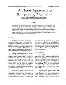
Figure 1 Sensitivity Analysis of Misclassification Costs

suggest that, in general, the MLPs trained with second-order algorithms have higher AUC valuesand lower misclassification costs, and can be fitted in lower time than those which use the traditional gradient descent algorithm. The model that yields the highest AUC values uses the Levenberg-Marquardt training algorithm (MLP 8), which has eighteen hidden nodes and whose sum squared error (SSE) is 0.165. However, considering the misclassification costs, the best model is that which employs the resilient back-propagation as its learning rule (MLP 10). Finally, as previously mentioned, the misclassification costs presented in Table 7 were calculated by considering a relative ratio of 1:5 (West, 2000). However, in the UK lending markets, the relative ratio of misclassification costs is dependent on the difference between retail interest rates and LIBOR rates. This dependency is due to the fact that Type I errors would lead the bank to miss out on these lending profits (retail interest rates minus LIBOR rates). Default risk has drastically changed in the past decade due, for instance, to the huge economic downturn and a massive number of business failures. Interest rates have changed vastly over the past 13 years and are now a fraction of what they were a decade ago.14 The LIBOR rates are now about 0.2% compared to about 6% in 2000 (at the time West′s paper was published). The relative ratio of misclassification costs is therefore likely to be far higher today. To address this change, a sensitivity analysis is conducted for a variety of ratios (1:1 to 1:100) in order to illustrate the performance of each model under these assumptions and threshold at which each model becomes optimal or, conversely, sub-optimal (see Figure 1). This will allow UK banks to make an estimate of their own corporate relative ratio of misclassification costs, and consult this sensitivity analysis to determine which model will perform optimally under their cost structure. As can be observed in Figure 1, the model with the lowest misclassification costs is MLP 10. The results of misclassification costs in Figure 1 are in consonance with the accuracy capacity of each default prediction model. Therefore, lenders should use those bankruptcy models which have higher performance in terms of 14

See http://www.fedprimerate.com/libor/libor_rates_history.htm


159

Table 8 Bankruptcy Models for Micro-Entities versus SME 2 with the U.K. Weights Model Training Sample

Validation Sample

AUC model AUC model AUC model AUC model microAltman et al. microAltman et al. entities (2010) entities (2010)

Models

Variables and statistical techniques

Model 1 (LR 1)

Financial variables / / Logistic regression

0.736

0.740

0.770

0.710

Model 2 (LR 2)

Financial and nonfinancial variables / / Logistic regression

0.809

0.800

0.806

0.750

Model 3 (MLP 10)

Financial and nonfinancial variables / / Multilayer perceptron

0.835

-

0.827

-

the AUC test and misclassification costs, independently of their costs associated with Type I-II errors. Therefore, in line with other authors (e.g. Angelini et al., 2008; Jagric et al., 2011; Neves and Vieira, 2006; Wilson and Sharda, 1994) we suggest that, in general, not only does the MLP have higher AUC values, but it has lower misclassification costs than the traditional LR approach. These empirical results confirm the theoretical superiority (principally, nonlinear and non-parametric adaptive-learning properties) in the development of bankruptcy models using the MLP over the parametric LR model. Therefore, we suggest that practitioners should explore the use of MLP-based models instead of the traditional parametric models since even a small improvement in the predictive accuracy of the MLP default prediction model is critical. In the case of banks, a 1% improvement in accuracy can reduce losses in a large loan portfolio and save millions of dollars (West, 2000). For other users (investors, managers and auditors), the improvement anticipates bankruptcy in a timely way, facilitating proactive management of loan portfolios to mitigate losses. In this sense, the results suggest that the difference between the best MLP in terms of misclassification costs (MLP 12) and LR (LR 2) is over 7.7% (see Table 7). This means that implementation of the neural network approach reduces bank losses significantly (7.73% exactly) and therefore constitutes a way to obtain a competitive advantage for those banks which implement this statistical technique. Finally, we examine whether the risk models designed specifically for subpopulation firms with large homogeneous characteristics (micro-entities) obtain higher predictability than those models built generically for the overall company population (SMEs). To this end, the model called SME 2 with the UK weights formulated by Altman et al. (2010) was chosen as the benchmark. The choice of this model is due to the fact that it is one of the few and most relevant studies involving the smallest SMEs. As can be observed in Table 8, the accuracy capacity obtained by the best bankruptcy model developed here specifically for micro-entities is higher than that attained by the model built for SMEs. Specifically, the improvement obtained by the selection of a more homogeneous company population is 5.60% in terms of the AUC for the models that consider only financial ratios (LR 1) and 6% for the models which introduce both financial and non-financial variables (LR 2).15 160


Moreover, when the multilayer perceptron technique is applied, the accuracy performance of the resulting model is still better, by 82.70% (see model MLP 10 of Table 8). Therefore, based on this empirical evidence, we suggest making risk models geared to the specific characteristic of the corporate sub-population, micro-entities in our case. Based on the above findings, we affirm that despite the significant improvement produced by the implementation of MLP-based models instead of use of the LR approach, (2.1% in terms of the AUC), the improvement resulting from the introduction of non-financial predictors is even higher (3.6% in terms of the AUC). This finding reinforces the idea that, in order to increase the predictive power of bankruptcy models, not only is the choice of statistical technique of major importance, but so are consideration of non-financial variables and selection of firms with very homogeneous characteristics (micro-entities in our case). In the latter case, i.e. consideration of micro-entities, the improvement is approximately 6% in terms of the AUC. It is the method that provides the most relevant improvement among the three lines of research conducted here (introduction of non-financial variables, implementation of the non-parametric statistical technique and selection of firms with homogeneous characteristics). 6. Concluding Remarks and Future Lines of Research In this paper we investigate the usefulness of parsimonious bankruptcy models developed for micro-entities based on multilayer perceptron neural networks and using both financial and non-financial variables. Our findings show three relevant conclusions. First, the parsimonious bankruptcy models developed specifically for micro-entities obtain greater predictive power than the most significant bankruptcy model built generically for the overall population of SMEs (the model called SME 2 with the UK weights created by Altman et al., 2010). Our results show an improvement of approximately 6% in terms of the AUC when bankruptcy models are developed specifically for micro-entities. It is therefore worth separating very small businesses from other companies when developing bankruptcy models since the improvement in the predictive capability justifies the potential difficulties in their implementation. This improvement in performance is particularly relevant in today’s climate of economic crisis, which has highlighted the inefficiency of current credit risk models in a business segment (micro-entities sector) with high rates of bankruptcy, excessive difficulty in accessing external funding; and significant impact on the GDP of the majority of developed economies. Moreover, the use of very few financial ratios (only five) constitutes a noteworthy improvement for the applicability and adaptation of our resulting failure models to the intrinsic characteristics of small businesses (with limited financial information). Second, the multilayer perceptron bankruptcy models can work to predict the bankruptcy of micro-entities, obtaining higher accuracy performance (in term of the AUC, test accuracy and Type I-II errors) and lower misclassification costs than the traditional LR approach. Therefore, bankruptcy prediction models, especially those developed under the ANN paradigm, constitute relevant tools that enable all 15

Both results are referred to the validation sub-sample.


161

the users to make better decisions by reducing the uncertainty associated with decision-making and, finally, by reducing the costs associated with bad business decisions. In the case of lenders, these findings have far-reaching consequences due to the added 7.7% cost savings that implementation of the best MLP model (MLP 12) yields here in comparison with the best LR model (LR 2). The MLP approach provides savings of millions of dollars and is therefore a means of obtaining a competitive advantage over those banks which implement traditional LR. Third, we find that the introduction of non-financial variables as predictors of business failure significantly improves the accuracy performance of models built specifically for micro-entities. Thanks to the introduction of non-financial predictors, the improvement, in terms of the AUC, is 3.6%, which is even higher than the improvement that involves the use of the best MLP (2.6%). Therefore, both the implementation of the neural network approach and the introduction of non-financial variables as predictors are two important means of improving the accuracy performance of bankruptcy prediction models for micro-entities. Thus, all stakeholders of micro-entities, particularly banks, creditors and shareholders, should carefully consider the results of this research for the detection of financial distress in firms of this size. In this sense, in a restrictive environment such as the one presented here, where viable investment projects planned by small firms cannot be carried out by weak and cautious financial intermediaries, our bankruptcy model provides an innovative paradigm not only for mitigation of the risk of a default occurring in the micro-entity segment, but also for improvement in such firms’ access to funding resources (mainly in the form of equity, bank debt and commercial debt). On the other hand, the models developed here can be useful for managers of micro-entities in analyzing internal problems and monitoring the performance of their companies by anticipating insolvency situations and taking steps to resolve them. Due to the very large dataset used here, both in the number of years (from 1999 to 2008) and in the number of enterprises (almost 40,000 sets of accounts of small firms), the contributions of this paper are relevant and useful for any small enterprise in any developed economy in the world. However, this study can be further improved in future research by using datasets of micro-entities from other countries and comparing their results with those obtained here. Yet another way to improve this work could be by collecting non-financial information of a more relevant nature for micro-entities, such as corporate governance variables, management skills and experience of company directors, features of auditors (such as the level of industry specialization), and the innovation capacity of firms, in order to increase the default prediction accuracy of our model. Finally, the statistical techniques used in this study can be compared with other non-parametric methods such as support vector machines, classification and regression trees, and random forest.

162


APPENDIX Table A1 Descriptive Statistics of the Quantitative Predictor Variables Variable

Failed

Non-Failed

Mean

Std. Desv.

Mean

Std. Desv.


0.45

1.32

1.77

4.95


0.12

0.23

0.06

0.17


3.24

5.55

2.45

5.40

-0.70

1.81

0.41

1.19

Net worth / Total assets Quick assets / Current assets

0.81

0.29

0.88

0.26

Cash / Net worth

4.55

5.66

2.91

4.59

Current assets / Current liabilities

1.17

2.56

2.35

4.31

Cash / Total assets

0.15

0.22

0.37

0.34

Retained profit / Total assets Trade creditors / Trade debtors

-0.56

1.43

0.01

0.03

6.67

17.25

12.66

22.84

Trade creditors / Total liabilities

0.84

0.27

0.85

0.30


0.43

0.31

0.31

0.31

Ln total assets Total assets Number oflegal claims

10.36 36,312.26

0.55 16,952.53

10.08 28,585.85

0.61 16,637.25

0.31

0.85

0.03

0.09

1,519.40

4,756.56

64.76

214.70

32.59

82.89

18.92

69.01

Ln age

7.48

0.68

7.51

1.08

Industry solvency

-0.07

0.24

0.18

0.52

Value of legal claims Late filing days


163

Table A2 Descriptive Statistics of the Qualitative Predictor Variables Variable

Category No (0)

Charge on asset Yes (1) No (0) Family firm Yes (1) No (0) Audited accounts Yes (1) No (0) Positive judgment audit report Yes (1) No (0) Negative judgment audit report Yes (1) No (0) Change auditor Yes (1)

Status

Frequency (%)

Failed

46.75

Non-Failed

49.40

Failed

3.25

Non-Failed

0.60

Failed

28.30

Non-Failed

25.56

Failed

21.70

Non-Failed

24.44

Failed

47.26

Non-Failed

48.14

Failed

2.74

Non-Failed

1.86

Failed

48.10

Non-Failed

48.32

Failed

1.90

Non-Failed

1.68

Failed

49.68

Non-Failed

49.89

Failed

0.32

Non-Failed

0.11

Failed

47.40

Non-Failed

47.63

Failed

2.60

Non-Failed

2.37

REFERENCES Angelini E, Tollo G di, Roli A (2008): A neural network approach for credit risk evaluation. Quarterly Review of Economics and Finance, 48(4):733–755. Altman EI (1968): Financial Ratios, Discriminant Analysis and Prediction of Corporate Bankruptcy. Journal of Finance, 23(4):589–609. Altman EI, Marco G, Varetto F (1994): Corporate Distress Diagnosis: Comparisons using Linear Discriminant Analysis and Neural Networks (the Italian experience). Journal of Banking and Finance, 18(3):505–529. Altman EI, Sabato G (2007): Modeling Credit Risk for SMEs: Evidence from US Market. A Journal of Accounting, Finance and Business Studies (ABACUS), 43(3):332-357. Altman EI, Sabato G, Wilson N (2010): The Value of Non-Financial Information in Small and Medium-Sized Enterprise Rrisk Management. Journal of Credit Risk, 6(2):95–127. Atiya AF (2001): Bankruptcy prediction for credit risk using neural networks: a survey and new results. IEEE Transactions on Neural Networks, 12(4):929–935. Beaver W (1966): Financial Ratios as Predictors of Failure, Empirical Research in Accounting: Selected Studied. Journal of Accounting Research, 4:71–111.

164


Berger AN, Frame SW (2007): Small Business Credit Scoring and Credit Availability. Journal of Small Business Management, 45(1):5–22. Bishop CM (1995): Neural Networks for Pattern Recognition. New York, Oxford University Press. Blanco A, Pino-Mejías R, Lara J, Rayo S (2013): Credit Scoring Models for the Microfinance Industry using Neural Networks: Evidence from Peru. Expert Systems with Applications, 40(1): 356–364. Boritz JE, Kennedy DB (1995): Effectiveness of Neural Network Types for Prediction of Business Failure. Expert Systems with Applications, 9(4):503–512. Chava S, Jarrow RA (2004): Bankruptcy Prediction with Industry Effects. Review of Finance, 8(4):537–569. Chen S, Härdle WK, Moro RA (2011): Modeling Default Risk with Support Vector Machines. Quantitative Finance, 11(1):135–154. Ciampi F, Gordini N (2013): Small Enterprise Default Prediction Modeling through Artificial Neural Networks: An Empirical Analysis of Italian Small Enterprises. Journal of Small Business Management, 51(1):23–45. Coats PK, Fant LF (1993): Recognizing Financial Distress Patterns Using a Neural Network Tool. Financial Management, 22(3):142–155. Crone SF, Finlay S (2012): Instance sampling in credit scoring: An empirical study of sample size and balancing. International Journal of Forecasting, 28(1):224–238. Dietsch M, Petey J (2004): Should SME Exposures Be Treated as Retail or Corporate Exposures? A Comparative Analysis of Default Probabilities and Asset Correlation in French and German SMEs. Journal of Banking and Finance, 28(4):773–788. Edmister R (1972): An Empirical Test of Financial Ratio Analysis for Small Business Failure Prediction. Journal of Financial and Quantitative Analysis, 7(2):1477–1493. Eisenbeis R (1977): Pitfalls in the application of discriminant analysis in business, finance, and economics. Journal of Finance, 32(3):875–900. Fletcher D, Goss E (1993): Forecasting with Neural Networks: An Application using Bankruptcy Data. Information and Management, 24(3):159–167. Gepp A, Kumar K, Bhattacharya S (2009): Business Failure Prediction using Decision Trees. Journal of Forecasting, 29:536–555. Grunert J, Norden L, Weber M (2005): The Role of Non-financial Factors in Internal Credit Ratings. Journal of Banking and Finance, 29(2):509–531. Hastie T, Tibshirani R, Friedman JH (2009): The Elements of Statistical Learning: Data Mining, Inference, and Prediction. New York, Springer Series in Statistics. Headd B (2003): Redefining Business Success: Distinguishing Between Closure and Failure. Small Business Economics, 21(1):51–61. Hudson J (1987): The Age, Regional and Industrial Structure of Company Liquidations. Journal of Business Finance and Accounting, 14(2):199–213. Ince H, Iktan B (2009): A comparison of data mining techniques for credit scoring in banking: a managerial perspective. Journal of Business Economics and Management, 10(3):233–240. Jagric V, Kracun D, Jagric T (2011): Does Non-linearity Matter in Retail Credit Risk Modeling? Finance a úvěr-Czech Journal of Economics and Finance, 61(4):384–402. Jones FL (1987): Current techniques in bankruptcy prediction. Journal of Accounting Literature, 6:131–164. Keasey K, Watson R (1987): Non-Financial Symptoms and the Prediction of Small Company Failure: A Test of Argenti’s Hypotheses. Journal of Business Finance and Accounting, 14(3):49–57. Lacher RC, Coats PK, Sharma S, Fant LF (1995): A Neural Network for Classifying the Financial Health of a Firm. European Journal of Operational Research, 85(1):53–65.


165

Moon T, Sohn S (2010): Technology credit scoring model considering both SME characteristics and economic conditions: The Korean case. Journal of the Operational Research Society, 61(4):666–675. Morten B, Nielsen KM, Perez-Gonzalez F, Wolfenzon D (2007): Inside the Family Firm: The Role of Families in Succession Decisions and Performance. Quarterly Journal of Economics, 122(2): 647–691. Neves JC, Vieira A (2006). Improving bankruptcy prediction with Hidden Layer Learning Vector Quantization. European Accounting Review, 15(2): 253–271. Official Journal of the European Union (2012): Directive 2012/6/EU of the European Parliament and of the Council, retrieved 10 January 2013. available at: http://eur-lex.europa.eu/LexUriServ/LexUriServ.do?uri=OJ:L:2012:081:0003:0006:EN:PDF Ohlson JA (1980): Financial Ratios and the Probabilistic Prediction of Bankruptcy. Journal of Accounting Research, 18(1):109–131. Peat M (2007): Factors Affecting the Probability of Bankruptcy: A Managerial Decision Based Approach. Abacus, 43(3):303–324. Peel MJ, Peel DA (1989): A Multilogit Approach to Predicting Corporate Failure—Some Evidence for the U.K. Corporate Sector. Omega International Journal of Management Science, 16(4): 309–318. Peel MJ, Peel DA, Pope PF (1986): Predicting Corporate Failure—Some Results for the UK Corporate Sector. Omega International Journal of Management Science, 14(1):5–12. Rayo S, Lara J, Camino D (2010): A Credit Scoring Model for Institutions of Microfinance under the Basel II Normative. Journal of Economics, Finance and Administrative Science, 15:89–124. Řezáč M, Řezáč F (2011): How to Measure the Quality of Credit Scoring Models. Finance a úvěrCzech Journal of Economics and Finance, 61(5):486–507. Rumelhart DE, Hinton DE, Williams RJ (1986): Learning Internal Representations by Error Propagation in Parallel Distributed Processing. Cambridge (MA), MIT Press. Taffler RJ (1984): Empirical Models for the Monitoring of UK Corporations. Journal of Banking and Finance, 8(2):199–227. Tascon M, Castano FJ (2012): Variables and Models for the Identification and Prediction of Business Failure: Revision of Recent Empirical Research Advances. Spanish Accounting Review, 15(1):7–58. West D (2000): Neural Network Credit Scoring Models. Computers and Operations Research, 27(11/12):1131–1152. Whittred GP, Zimmer I (1984): Timeliness of Financial Reporting and Financial Distress. Accounting Review, 59(2):297–295. Wilson N, Altanlar A (2014): Company Failure Prediction with Limited Information: Newly Incorporated Companies. Journal of the Operational Research Society, 65(2):252–264. Zhang GP, Patuwo BE, Hu MY (1998): Forecasting with Artificial Neural Networks: The State of the Art. International Journal of Forecasting, 14(1):35–62. Zmijewski ME (1984): Methodological Issues Related to the Estimation of Financial Distress Prediction Models. Journal of Accounting Research, 22(Suppl.):59–82.

166


Improving Bankruptcy Prediction in Micro-Entities by Using Nonlinear ...

Improving Bankruptcy Prediction in Micro-Entities by Using Nonlinear ...

Suggest Documents

Companies Bankruptcy Prediction by Using Altman ... - CiteSeerX

Bankruptcy Prediction of Financially Distressed Companies using

Machine Learning Methods of Bankruptcy Prediction Using ...

Bankruptcy Prediction Using Machine Learning - Scientific Research

Bankruptcy Prediction Using Data Mining ...

High-Performance Bankruptcy Prediction Model using ...

Early bankruptcy prediction using ENPC - Core

Bankruptcy Prediction of Financially Distressed Companies using

Early Warning System for Bankruptcy: Bankruptcy Prediction

Early Warning System for Bankruptcy: Bankruptcy Prediction

Early Warning System for Bankruptcy: Bankruptcy Prediction

Nonlinear Prediction by Reinforcement Learning

bankruptcy prediction of engineering companies in the eu using

Bankruptcy Prediction Models: Can the Prediction ...

neural networks in bankruptcy prediction - Core

PREDICTION OF CORPORATE BANKRUPTCY

Apply Logit analysis in Bankruptcy Prediction - CiteSeerX

selection of predictors in bankruptcy prediction ...

Bankruptcy Prediction - The Clute Institute

Improving Protein-Protein Interaction Prediction by Using ... - waset

Improving Market Clearing Price Prediction by Using a ... - CiteSeerX

Improving word prediction for augmentative communication by using ...

A Genetic Programming Approach for Bankruptcy Prediction Using a ...

Bankruptcy prediction using support vector machine with ... - CiteSeerX