Improving Context-Based Load Value Prediction - Computer Science ...

Improving Context-Based Load Value Prediction by

Martin Burtscher Dipl.-Ing., Eidgenössische Technische Hochschule, 1996

A thesis submitted to the Faculty of the Graduate School of the University of Colorado in partial fulfillment of the requirement for the degree of Doctor of Philosophy Department of Computer Science 2000

© 2000 Martin Burtscher

This thesis entitled: Improving Context-Based Load Value Prediction written by Martin Burtscher has been approved for the Department of Computer Science

Benjamin G. Zorn

Michael Franz

Dirk Grunwald

William M. Waite

James H. Martin

Date

The final copy of this thesis has been examined by the signatories, and we find that both the content and the form meet acceptable presentation standards of scholarly work in the above mentioned discipline.

Burtscher, Martin (Ph.D., Computer Science) Improving Context-Based Load Value Prediction Thesis directed by Associate Professor Benjamin G. Zorn

Abstract Microprocessors are becoming faster at such a rapid pace that other components like random access memory cannot keep up. As a result, the latency of load instructions grows constantly and already often impedes processor performance. Fortunately, load instructions frequently fetch predictable sequences of values. Load value predictors exploit this behavior to predict the results of load instructions.

Because the predicted values are available before the

memory can deliver the true load values, the CPU is able to speculatively continue processing without having to wait for memory accesses to complete, which improves the execution speed. The contributions of this dissertation to the area of load value prediction include a novel technique to decrease the number of mispredictions, a predictor design that increases the hardware utilization and thus the number of correctly predicted load values, a detailed analysis of hybrid predictor combinations to determine components that complement each other well, and several approaches to substantially reduce the size of hybrid load value predictors without affecting their performance. One result of this research is a very small yet high-performing load value predictor. Cycle-accurate simulations of a four-way superscalar microprocessor running SPECint95 show that this predictor outperforms other predictors from the literature by twenty or more percent over a wide range of sizes. With about fifteen kilobytes of state, the smallest examined configuration, it surpasses the speedups delivered by other, five-times larger predictors both with a re-fetch and a re-execute misprediction recovery mechanism. iv

Dedication

To my family.

Acknowledgements

Many wonderful people have helped me succeed in academics and life. First and foremost, I would like to thank my mother, whose never-ending encouragement, patience, and help doubtlessly brought me to where I am today, and my father, who motivated and supported my interest in computers and sciences a great deal. Many teachers have made lasting positive impressions on me and have provided invaluable guidance. Most importantly, it has been a great experience and pleasure to work with my advisor Professor Benjamin Zorn, whose help, support, and insights I am extremely grateful for. He always knew how and when to guide me while still allowing me immense freedom and flexibility with my work, which I appreciate very much. But also Professors Michael Franz, Dirk Grunwald, Amer Diwan, William Waite, and James Martin, as well as my fellow students and many other great people have shaped my career and success to no small amount. I would like to especially thank my fiancée Anna Szczyrba for her encouragement and support of my work and for bearing with me all this time. This work was funded in part by the Hewlett Packard University Grants Program (including Gift No. 31041.1) and the Colorado Advanced Software Institute. I would like to thank Tom Christian for his support of this project and Dirk Grunwald and Abhijit Paithankar for providing and helping with the cycle-accurate simulator. In addition to using Hewlett Packard desktop computers, most of the simulations were performed on Alpha machines, which were sponsored by a Digital Equipment Corporation (now Compaq) grant.

vi

Contents CHAPTER 1 .................................................................................................. 1 1 INTRODUCTION........................................................................................ 1 1.1 PROBLEM ......................................................................................... 1 1.2 LOAD VALUE LOCALITY ...................................................................... 3 1.3 PREDICTION APPROACHES ................................................................ 4 1.4 CONFIDENCE ESTIMATION.................................................................. 5 1.5 CONTRIBUTIONS ............................................................................... 6 1.6 SUMMARY ........................................................................................ 9 1.7 ORGANIZATION ................................................................................. 9 CHAPTER 2 ................................................................................................ 10 2 BACKGROUND........................................................................................ 10 2.1 CONVENTIONAL HIGH-PERFORMANCE PROCESSOR ARCHITECTURE .... 10 2.2 MISPREDICTION RECOVERY MECHANISMS......................................... 14 2.3 SUMMARY ...................................................................................... 15 CHAPTER 3 ................................................................................................ 17 3 EVALUATION METHODS........................................................................ 17 3.1 BASELINE ARCHITECTURE ............................................................... 17 3.2 BENCHMARKS ................................................................................. 20 3.2.1 General Information ............................................................... 20 3.2.2 Quantile Information .............................................................. 22 3.2.3 Segment Information ............................................................. 24 3.2.4 Segment Quantile Information ............................................... 26 3.3 SPEEDUP ....................................................................................... 27 3.4 OTHER METRICS ............................................................................. 29 vii

3.5 SUMMARY ...................................................................................... 32 CHAPTER 4 ................................................................................................ 33 4 CONTEXT-BASED VALUE PREDICTORS.............................................. 33 4.1 CONTEXT-BASED VALUE PREDICTION ............................................... 33 4.2 GENERIC CONTEXT-BASED LOAD VALUE PREDICTOR ........................ 34 4.3 FIVE CONTEXT-BASED LOAD VALUE PREDICTORS ............................. 36 4.3.1 Last Value Predictor “LV”....................................................... 36 4.3.2 Register Predictor “Reg” ........................................................ 38 4.3.3 Stride 2-delta Predictor “St2d” ............................................... 39 4.3.4 Last Four Value Predictor “L4V” ............................................ 43 4.3.5 Finite Context Method Predictor “FCM” ................................. 44 4.4 PREDICTOR PERFORMANCE ............................................................. 47 4.5 SUMMARY ...................................................................................... 48 CHAPTER 5 ................................................................................................ 49 5 CONFIDENCE ESTIMATORS ................................................................. 49 5.1 THE NEED FOR CONFIDENCE ESTIMATORS........................................ 49 5.2 THE BIMODAL CONFIDENCE ESTIMATOR ........................................... 50 5.2.1 Behavior Study ...................................................................... 53 5.3 THE SAG CONFIDENCE ESTIMATOR .................................................. 56 5.4 PERFORMANCE COMPARISON .......................................................... 60 5.4.1 The L4V Selector ................................................................... 65 5.4.2 Other Performance Metrics.................................................... 66 5.5 SUMMARY ...................................................................................... 70 CHAPTER 6 ................................................................................................ 72 6 PREDICTOR BANKING ........................................................................... 72 6.1 THE NEED FOR BANKING ................................................................. 72 6.2 BANK ARCHITECTURE...................................................................... 73 viii

6.3 BANK PERFORMANCE ...................................................................... 76 6.4 BANK USAGE .................................................................................. 79 6.5 SUMMARY ...................................................................................... 79 CHAPTER 7 ................................................................................................ 81 7 IMPROVING PREDICTOR UTILIZATION................................................ 81 7.1 LINE UTILIZATION ............................................................................ 81 7.2 TRADING OFF HEIGHT FOR W IDTH .................................................... 83

7.3 SAG L4V PREDICTOR DESIGN AND PERFORMANCE ........................... 84 7.4 SAG L4V PREDICTOR POTENTIAL .................................................... 87 7.4.1 Comparison with Oracles....................................................... 88

7.5 SAG L4V SENSITIVITY ANALYSIS ..................................................... 91 7.5.1 SAg History Length................................................................ 91 7.5.2 SAg Counter Parameters....................................................... 93 7.5.3 Optimizing Individual Programs ............................................. 95 7.5.4 Using Distinct Last Values ................................................... 100 7.6 SUMMARY .................................................................................... 104 CHAPTER 8 .............................................................................................. 105 8 HYBRIDIZING LOAD VALUE PREDICTORS ........................................ 105 8.1 THE BENEFIT OF HYBRIDIZATION .................................................... 105 8.2 HYBRID PERFORMANCE ................................................................. 106 8.3 SHARED AND UNIQUE PERFORMANCE CONTRIBUTIONS .................... 114 8.3.1 Two-component Hybrids...................................................... 114 8.3.2 Three-component Hybrids ................................................... 118 8.4 SUMMARY .................................................................................... 120 CHAPTER 9 .............................................................................................. 122 9 HYBRIDIZING WITH HARDWARE REUSE........................................... 122 9.1 SHRINKING THE REG+ST2D+L4V HYBRID ...................................... 122 ix

9.1.1 Shrinking the L4V Component............................................. 123 9.1.2 Making the Stride Predictor Storage-less ............................ 125 9.2 COALESCING HYBRID PREDICTOR COMPONENTS ............................. 127 9.3 THE COALESCED-HYBRID .............................................................. 127 9.4 COALESCED-HYBRID PERFORMANCE .............................................. 129 9.4.1 Comparison with Other Predictors ....................................... 129 9.4.2 Comparison with Oracles..................................................... 135 9.5 COALESCED-HYBRID SENSITIVITY ANALYSIS ................................... 137 9.5.1 Component Permutations .................................................... 138 9.5.2 Tags and B-Tags ................................................................. 139 9.5.3 Predictor Width .................................................................... 140 9.6 SUMMARY .................................................................................... 142 CHAPTER 10 ............................................................................................ 144 10 RELATED WORK ................................................................................ 144 10.1 EARLY W ORK ............................................................................. 144 10.2 PREDICTORS .............................................................................. 145 10.3 PROFILE-BASED APPROACHES ..................................................... 146 10.4 OTHER RELATED W ORK .............................................................. 147 10.4.1 Dependence Prediction ..................................................... 151 10.4.2 Confidence Estimation....................................................... 151 10.4.3 Branch Prediction .............................................................. 152 CHAPTER 11 ............................................................................................ 153 11 SUMMARY AND CONCLUSIONS ....................................................... 153 APPENDIX ................................................................................................ 162 12 APPENDIX ........................................................................................... 162

x

Tables TABLE 3.1: FUNCTIONAL UNIT AND MEMORY LATENCIES (IN CYCLES). ......................... 18 TABLE 3.2: INFORMATION ABOUT THE SPECINT95 BENCHMARK SUITE. ...................... 21 TABLE 3.3: SPECINT95 QUANTILE INFORMATION. ..................................................... 23 TABLE 3.4: INFORMATION ABOUT THE EIGHT SIMULATED PROGRAM SEGMENTS. .......... 24 TABLE 3.5: QUANTILE INFORMATION ABOUT THE SIMULATED PROGRAM SEGMENTS...... 26 TABLE 4.1: LAST VALUE, STRIDE, AND STRIDE 2-DELTA LOAD VALUE LOCALITY............ 41 TABLE 5.1: BEHAVIOR STUDY OF A BIMODAL CONFIDENCE ESTIMATOR. ....................... 54 TABLE 5.2: HISTORY-PATTERN FREQUENCY AND LAST VALUE PREDICTABILITY. ........... 57 TABLE 5.3: BIMODAL AND SAG CE BEHAVIOR ON THREE GCC TRACES. ...................... 61 TABLE 5.4: PREDICTOR CONFIGURATIONS YIELDING THE HIGHEST MEAN SPEEDUP. ..... 63 TABLE 5.5: LATENCY AND CYCLES TO FIRST USAGE OF THE PREDICTED LOAD VALUES. 68 TABLE 5.6: VARIOUS METRICS SHOWING ANOMALY. .................................................. 69 TABLE 7.1: BEST INDIVIDUAL AND AVERAGE PREDICTOR CONFIGURATIONS. ................ 98 TABLE 7.2: THE L4V SPEEDUP OF GCC FOR DIFFERENT PENALTY VALUES. ................. 99 TABLE 7.3: THE L4V SPEEDUP OF GCC FOR DIFFERENT THRESHOLD VALUES.............. 99 TABLE 8.1: THE CONFIDENCE ESTIMATOR PARAMETERS OF THE HYBRID PREDICTORS.108 TABLE 8.2: RE-FETCH SPEEDUP BENEFIT FROM ADDING COMPONENTS. .....................113 TABLE 8.3: RE-EXECUTE SPEEDUP BENEFIT FROM ADDING COMPONENTS. .................113 TABLE 9.1: STATE REQUIREMENT OF THE SEVEN PREDICTORS’ THREE CONFIGURATIONS. .....................................................................................................................131 TABLE 9.2: THE BASE-CONFIGURATIONS OF THE SEVEN PREDICTORS.......................132 TABLE 9.3: SPEEDUP OF THE SIX MAIN COMPONENT PERMUTATIONS. ........................138 TABLE 12.1: BANKING INFORMATION. ......................................................................166

xi

Figures FIGURE 2.1: THE EXECUTION PIPELINE OF A HIGH-PERFORMANCE MICROPROCESSOR. 12 FIGURE 3.1: THE FOUR PREDICTION CLASSIFICATIONS. ............................................. 30 FIGURE 4.1: THE COMPONENTS OF A CONTEXT-BASED LOAD VALUE PREDICTOR. ........ 34 FIGURE 4.2: THE LAST VALUE PREDICTOR. ............................................................... 37 FIGURE 4.3: THE REGISTER PREDICTOR. .................................................................. 38 FIGURE 4.4: AVERAGE RUN-LENGTH OF SEQUENCES OF REPEATING LOAD VALUES...... 40 FIGURE 4.5: THE STRIDE 2-DELTA PREDICTOR. ......................................................... 42 FIGURE 4.6: THE LAST FOUR VALUE PREDICTOR. ...................................................... 43 FIGURE 4.7: THE FINITE CONTEXT METHOD PREDICTOR. ............................................ 46 FIGURE 4.8: MEAN SPEEDUP OF FIVE CONTEXT-BASED PREDICTORS. ......................... 47 FIGURE 5.1: THE BIMODAL CONFIDENCE ESTIMATOR (SHADED). ................................. 52 FIGURE 5.2: THE SAG CONFIDENCE ESTIMATOR (SHADED). ....................................... 59 FIGURE 5.3: RE-FETCH SPEEDUP COMPARISON BETWEEN BIMODAL AND SAG CES..... 64 FIGURE 5.4: RE-EXECUTE SPEEDUP COMPARISON OF BIMODAL AND SAG CES. .......... 64 FIGURE 5.5: LOAD CLASSIFICATION OF BIMODAL AND SAG CONFIDENCE ESTIMATORS. 67 FIGURE 6.1: LINE CORRESPONDENCE OF SINGLE-BANK AND INTERLEAVED PREDICTOR.74 FIGURE 6.2: RE-FETCH SPEEDUP OF DIFFERENTLY BANKED SAG PREDICTORS. .......... 76 FIGURE 7.1: ABSOLUTE QUANTILE NUMBERS FOR THE EIGHT SPECINT95 PROGRAMS. 82 FIGURE 7.2: RE-FETCH SPEEDUP OF THREE SIZES OF LAST N VALUE PREDICTORS....... 86 FIGURE 7.3: RE-EXECUTE SPEEDUP OF THREE SIZES OF LAST N VALUE PREDICTORS... 86 FIGURE 7.4: PERFORMANCE OF L4V PREDICTORS WITH DIFFERENT ORACLES. ........... 89 FIGURE 7.5: MEAN SPEEDUP WITH DIFFERENT HISTORY LENGTHS. ............................. 92 FIGURE 7.6: BEST L4V PERFORMANCE FOR DIFFERENT SATURATING-COUNTER SIZES. 94 FIGURE 7.7: THE SPEEDUP OF THE SPECINT95 PROGRAMS USING RE-FETCH. ........... 96 FIGURE 7.8: THE SPEEDUP OF THE SPECINT95 PROGRAMS WITH RE-EXECUTE. ......... 96 FIGURE 7.9: THE AVERAGE LAST N VALUE AND LAST DISTINCT N VALUE PREDICTABILITY. .....................................................................................................................101 FIGURE 7.10: SPEEDUP OF THE TAG SAG L4V AND THE TAG SAG LD4V. .................103 FIGURE 8.1: HYBRID PERFORMANCE USING RE-FETCH..............................................107 FIGURE 8.2: HYBRID PERFORMANCE USING RE-EXECUTE..........................................110

xii

FIGURE 8.3: RE-EXECUTE AND RE-FETCH VENN-DIAGRAMS FOR SAG HYBRIDS. .........115 FIGURE 8.4: RE-EXECUTE AND RE-FETCH VENN-DIAGRAMS FOR BIMODAL HYBRIDS. ...117 FIGURE 8.5: VENN-DIAGRAMS FOR SAG-BASED THREE-COMPONENT HYBRIDS. ..........119 FIGURE 9.1: THE ARCHITECTURE OF THE COALESCED-HYBRID LOAD VALUE PREDICTOR. .....................................................................................................................128 FIGURE 9.2: RE-FETCH SPEEDUP OF SEVERAL PREDICTORS FOR THREE SIZES...........133 FIGURE 9.3: RE-EXECUTE SPEEDUP OF SEVERAL PREDICTORS FOR THREE SIZES.......133 FIGURE 9.4: PERFORMANCE OF DIFFERENT COALESCED-HYBRID ORACLES. ...............136 FIGURE 9.5: THE COALESCED-HYBRID’S SPEEDUP WITH VARIOUS TAG SCHEMES........139 FIGURE 9.6: PERFORMANCE WITH DIFFERENT LAST N PARTIAL VALUE COMPONENTS. .141 FIGURE 12.1: RE-FETCH SPEEDUP OF DIFFERENTLY BANKED BIMODAL PREDICTORS...164 FIGURE 12.2: RE-EXECUTE SPEEDUP OF DIFFERENTLY BANKED BIMODAL PREDICTORS. .....................................................................................................................165 FIGURE 12.3: RE-EXECUTE SPEEDUP OF DIFFERENTLY BANKED SAG PREDICTORS.....165 FIGURE 12.4: THE RE-FETCH SPEEDUP MAPS FOR THE FIVE BASIC SAG PREDICTORS. 167 FIGURE 12.5: RE-EXECUTE SPEEDUP MAPS FOR THE FIVE BASIC SAG PREDICTORS. ..168

xiii

Chapter 1 1 Introduction Introduction

This chapter describes how the slow execution speed (the latency) of load instructions can impact the performance of a processor and introduces load value prediction, a promising approach to alleviate the load latency problem. Furthermore, the contributions of this dissertation to the area of load value prediction are presented.

1.1 Problem Processor technology is advancing at a rapid pace. Over the past two decades the CPU speed has roughly doubled every one and a half years (this is informally known as Moore’s Law). To continue this trend and to satisfy the incessantly growing need for more computing power, novel techniques are needed to make microprocessors faster and faster.

This dissertation ex-

plores and improves one such technique called load value prediction. While the CPU performance has been accelerating at a high speed, the advances in other areas (such as the reduction of the memory latency) have not been as dramatic. As a consequence, memory accesses have in relative terms become slower over the years and have reached a point where they present one of the biggest processor performance bottlenecks. Load value prediction reduces the effective memory latency and thus speeds up the CPU. Load instructions copy data from memory to a register inside the CPU. The register that receives the data is called the target register and is specified 1

in the load instruction. Registers can be accessed very rapidly, but a CPU can only have relatively few of them (usually fewer than about sixty-four). The memory, on the other hand, can hold over a million times more data than the register file but accessing it takes on the order of a hundred times longer, making such accesses very time consuming. To reduce the access time of frequently used data, most computers incorporate levels of fast cache memory. The first cache level (L1) is normally the smallest but also the fastest and temporarily stores the most recently used data in case it is needed again. Consecutive levels are larger and slower. The main memory is at the end of the (volatile) memory hierarchy and has the longest access time. When a load instruction is executed, the caches are successively queried until the desired data item is found. If the L1 cache contains that data, the load value will be available quickly. If the data cannot be found in any cache, the data has to be retrieved from the main memory. Hence, the time it takes to execute a load instruction depends on the cache level that satisfies the load request and can vary from a few cycles to over a hundred cycles. In comparison, reading a value from the CPU’s register file never takes longer than one cycle. Because the technological enhancements have improved CPUs more than memory chips, the speed-gap between CPU and memory grows constantly, making load instructions slower and slower relative to the CPU. If this trend continues, and there is currently no indication that it will not, the load latency will become even longer and more of a problem in the future. Load instructions belong to the most frequently executed instructions. Many programs, even highly optimized ones, execute more than one load for every five executed instructions [LCB+98]. Hence, the latency of load instructions can, and frequently does, hamper system performance. Conversely, reducing the (effective) load latency has the potential to substantially speed up program execution. Only branch instructions present a similarly substantial source of over-

2

head in modern microprocessors. While extensive research has been performed to alleviate the performance impact of branches (for example by using sophisticated branch predictors [LCM97], branch target buffers [PeSm93], and return address stacks [KaEm91]), relatively little has been done to address the load latency problem. As opposed to load instructions, latency is not an issue with store instructions because their (slow) memory access takes place “after” the execution of the store, i.e., the CPU can proceed without having to wait for the store to complete. Write buffers [Jou93] perform the actual store operation at some later time and make sure that consistency is maintained. Unfortunately, nothing similar can be done for load instructions because the fetched values are often almost instantly needed by the immediately following instructions. These instructions cannot execute before the load they depend on has completed. Even worse, all the indirectly dependent instructions are also delayed until the load has completed.

1.2 Load Value Locality Fortunately, load instructions often fetch predictable sequences of values [LWS96].

For instance, about half of all the load instructions in the

SPECint95 benchmark suite retrieve the same value that they did the previous time they were executed. Such behavior, which has been demonstrated explicitly on a number of architectures, is referred to as value locality [Gab96, LWS96]. The predictability of load values can be exploited by predicting the result of a load instruction before the memory can provide the load value. Several distinct types of load value locality have been identified so far and predictors to exploit them have been proposed [BuZo99b, Gab96, LWS96, SaSm97b, TuSe99, WaFr97]. The main goal of this dissertation is to develop and evaluate new and better performing load value predictors. If load values are predicted quickly and correctly, the CPU is able to con3

tinue processing the dependent instructions without having to wait for the memory access to finish. Of course it is only known whether a prediction was correct once the true value has been retrieved from memory, which can take many cycles. Speculative execution allows the CPU to continue execution with a predicted value before the prediction outcome is known [John91]. If it later turns out that the prediction was correct, the speculative status can simply be dropped. If the prediction was incorrect, everything that the CPU did using the incorrect value has to be purged and redone with the correct value. Because branch predictors require a similar mechanism to recover from mispredictions, most modern CPUs already contain the necessary hardware to perform this kind of speculation [Gab96]. However, recovering from mispredictions takes time and slows down the processor. Load value prediction therefore only makes sense if the predictions are often correct. Improving the accuracy of load value predictions is another goal of this thesis. Empirically, papers have shown that the results of most instructions are predictable [Gab96, LiSh96, SaSm97a]. While predicting the result of every instruction potentially enables wide issue CPUs to exceed the existing instruction level parallelism (ILP) [GaMe98, LiSh96], predicting only load values requires substantially less and simpler hardware while still yielding most of the performance potential found in value prediction [ReCa98], and can even be advantageous in single-issue CPUs.

1.3 Prediction Approaches There are three basic ways to find predictable load instructions and to determine their load values. The first possibility is static prediction. This approach makes all decisions prior to program execution. Hence, the only information available is the binary, predefined heuristics, and possibly the source code. Profile-based approaches represent another possibility. They measure and record the behavior of programs for several sample inputs. Fi4

nally, dynamic approaches continuously measure the behavior of programs while they are executing. The static approach is rather limited due to the large number of runtime constants whose values are not known at compile time [CFE97]. Profiling often suffers from insufficient coverage, i.e., not all parts of a program are executed during the profile run, which means that no information for those parts is gathered.

Furthermore, both static and profile-based approaches need

support in the instruction set architecture (ISA) to communicate information to the hardware. Such support is generally not available in existing CPU families. The dynamic approach does not suffer from these problems, but it requires a predictor to be present in hardware. Furthermore, the dynamic approach does not know a priori which load instructions are predictable, meaning that space has to be provided in the predictor for both predictable and unpredictable loads. Hence, it may be advantageous to combine a static or profile-based approach with a dynamic predictor to filter out the unpredictable loads so that the predictor only has to be designed large enough to handle the predictable loads [GaMe97]. Another important advantage of the dynamic approach is that it can adapt to changes in the program behavior during the course of the execution. The information provided by static approaches or by profiles is normally fixed and cannot be changed at runtime. Due to the limitations of the static and the profile-based approaches, I will restrict my investigation to dynamic, hardware-based load value predictors that are completely transparent (i.e., do not require changes to the ISA) and can therefore be added to existing as well as future microprocessors. No profiling or compiler support is needed for my predictors.

1.4 Confidence Estimation Thirty to fifty percent of the executed load instructions cannot be correctly 5

predicted with the currently known prediction techniques. Trying to predict these loads will inevitably result in mispredictions. Because recovering from mispredictions takes time, a high misprediction-rate can incur a recovery cost that eradicates any benefit that was gained from the correct predictions. Hence, it is possible for a load value predictor to slow down the processor instead of speeding it up. To keep the number of mispredictions at a minimum, almost all load value predictors incorporate some form of confidence estimator that tries to identify predictions that are likely to be incorrect so that they can be inhibited. Inhibiting such predictions reduces the number of mispredictions (and the associated recovery cost) and thus improves the predictor’s performance. This dissertation presents a new confidence estimator that makes fewer mispredictions than the conventional confidence estimator and therefore results in more effective load value predictors.

1.5 Contributions The goal of this dissertation is to develop and evaluate methods for context-based load value prediction, that is, to enhance various aspects of transparent, hardware-based load value predictors. My contributions towards this goal include the following: • Fewer mispredictions The development of an improved confidence estimator that decreases the number of mispredictions and consequently increases the performance of load value predictors • Better hardware utilization The design of a load value predictor that allocates more hardware to the frequently executed loads, which improves the predictor utilization and results in more load instructions being correctly predicted 6

• Hybrid analysis The analysis of a large number of hybrid predictor combinations to determine components that complement each other well and thus yield high-performing hybrid load value predictors • Size reduction techniques Several approaches to substantially reduce the size of hybrid load value predictors by sharing large amounts of state between their components, which decreases the predictor size while maintaining the performance

One direct result of this research is a high-performing load value predictor that includes all of the above mentioned enhancements. It is a hybrid of wellcomplementing components that is very small due to the large degree of state sharing. With about fifteen kilobytes of state, it outperforms five-times larger predictors from the literature. Among predictors of similar size, my predictor outperforms others by twenty or more percent over a large range of predictor sizes. The individual contributions are discussed in a little more detail in the following paragraphs. Analyzing the performance of an existing confidence estimator revealed a weakness that prevents it from correctly handling sequences of alternating predictability, which represent an important subset of the predictable load value sequences. To alleviate this problem, I developed a more complex confidence estimator that is somewhat larger but yields on average ten percent more performance in connection with most load value predictors. Moreover, there is evidence that the new confidence estimator embodies a better selector for hybrid load value predictors, improving the performance even further over the conventional confidence estimator. An investigation of the utilization of the hardware in a basic load value predictor revealed that most parts of the predictor are hardly ever or never used while a small part is used extremely frequently. To improve the utilization, I studied possible rearrangements of the predictor’s hardware. I found

7

an arrangement that allocates more hardware to the frequently executed load instructions and that is therefore able to correctly predict a larger number of loads, which improves the average predictor performance by about ten percent. Then I noticed that many of the values this improved predictor retains differ only by a small amount. This allowed me to devise a predictor in which the values are stored in a compressed format. Compressing the values reduces the predictor size by about one half while essentially maintaining the predictor’s performance. Next I discovered that components of hybrid predictors frequently store the same information. Hence, the redundant information can be eliminated, which can reduce the size of hybrids by more than a factor of two without compromising the predictor’s performance. A detailed component analysis of a large number of predictor combinations revealed some unexpected results. For example, powerful individual components frequently do not complement each other well in a hybrid configuration. Conversely, some components that perform rather poorly when used in isolation can form strong coalitions with other components. The results of this analysis allowed me to design a hybrid out of components that are small yet complement each other well. Many other hybrid predictors were found to contain components that predict highly overlapping sets of load instructions and therefore do not ideally complement one another. Furthermore, some hybrids actually yield a lower performance than their individual components due to negative interference. Finally, this dissertation presents performance numbers for a large number of load value predictors that are all evaluated in the same environment (i.e., the same simulator, the same benchmark programs, etc.), making it possible to truly compare the predictors. Furthermore, various performance metrics are introduced and studied, and a simple predictor banking scheme is evaluated.

8

1.6 Summary One of the largest performance bottlenecks in current microprocessors is the growing load latency. Load value prediction has the potential to substantially reduce the load latency. The main contribution of this dissertation is the development and evaluation of a high-performing yet relatively small load value predictor that significantly outperforms other predictors from the literature.

1.7 Organization The remainder of this dissertation is organized as follows. Chapter 2 explains the impact of the load latency on modern superscalar CPUs as well as the operation of two misprediction recovery mechanisms.

Chapter 3 de-

scribes the configuration of the simulator that is used to measure the speedup numbers and discusses the benchmarks and their load value locality. Chapter 4 introduces the architecture of five basic load value predictors. Chapter 5 investigates two confidence estimation schemes. Chapter 6 analyzes the performance of predictor banking. Chapter 7 takes a closer look at the utilization of the predictor hardware and proposes an improved design. Chapter 8 evaluates a large number of predictor combinations to build well performing hybrids. Chapter 9 improves the results from Chapter 8 by investigating ways to shrink the size of predictors through hardware reuse. Chapter 10 presents related work. Chapter 11 summarizes my work and takes a look into the future.

9

Chapter 2 2 Background Background

This chapter provides background on several features of highperformance microprocessors, including parallel instruction execution (superscalar execution), the dynamic re-sequencing of the execution order of independent instructions (out-of-order execution), and their interaction with load value predictors. Two misprediction recovery mechanisms are presented. The first one, which is the one that is also used for recovering from branch mispredictions, is already implemented in current processors but does not yield the best performance in combination with load value predictors. This is why a better, not yet implemented alternative is also discussed.

2.1 Conventional High-Performance Processor Architecture Most of today’s high-performance microprocessors are superscalar and have built-in hardware support for speculative and out-of-order execution [Edm+95, Half95, Yeag96, You94]. Since it is my goal to improve the performance of a high-end microprocessor, all the performance numbers presented in this dissertation are based on such a CPU. The specifications of the actual processor that is used for these measurements are described in Section 3.1. A superscalar CPU is capable of executing more than one instruction at a time. Out-of-order execution refers to the ability to dynamically adjust the order in which instructions are executed to increase the utilization of the avail10

able hardware and thus to improve the performance. Speculative execution is execution that can be undone if necessary. Having this ability makes it possible to process instructions whose execution and/or input values are based on a guess (such as a predicted branch outcome or a predicted load value) because it may later be necessary to undo the execution of such instructions if the guess turns out to be incorrect. Only the execution-core of a processor usually handles instructions out-oforder. Instruction fetch, decode, rename, and retirement is performed inorder [SmSo95] because dependencies are either not known in these pipeline stages or need to be handled in-order to facilitate correct execution. Instructions are retired in-order to support precise exceptions, to be able to replay instructions, and to enforce sequential semantics. Register renaming removes false dependencies from the in-flight instructions by dynamically mapping the logical registers to a larger set of physical registers, thus ensuring that instructions that have their input operands available are truly independent and can therefore be executed in any order or even in parallel with all other ready instructions. The renamed instructions are (at least conceptually) fed into the CPU’s instruction window as long as there are slots available. An inserted instruction remains in this window in a waiting state until all of its source operands are available.

Once all the inputs are obtained, the instruction becomes

ready, i.e., eligible for execution. The CPU’s issue logic continuously scans the instruction window for such instructions. If a ready instruction is found and a functional unit capable of executing that type of instruction is available, the issue logic assigns the instruction to the functional unit for execution. At this point, the instruction is marked as executing. Once the functional unit has completed the execution, the result is stored and forwarded to the waiting instructions, making them ready if the current result was the last input operand they were waiting for. Completed instructions are marked as done. Only instructions marked as done can be retired (or committed) from the instruc-

11

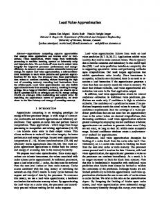
tion window. Superscalar processors are able to locate and issue multiple ready instructions per cycle (with a fixed upper limit), as long as there are enough functional units (FUs) and ready instructions available. In addition, they are able to forward multiple results per cycle to waiting instructions. Most of the FUs in high-performance CPUs are either pipelined (i.e., they can start executing a new instruction every cycle) or they only have a onecycle latency. The most frequently used FUs are often duplicated for faster execution. Figure 2.1 shows the described pipeline stages, the instruction window, the issue logic, and several functional units. The instruction window contains some sample instructions in different stages of execution (i.e., waiting, ready, executing, and done).

Actual CPU implementations may vary

from this diagram (for example, most processors contain more slots in the instruction window than are depicted).

Instruction Window retire/commit

done add r2 := r2+1

ready add r1 := r1+r3

done bne r2 != end

exec load r3 := [r2]

add r1 := r1+r3

done add r2 := r2+1

wait

exec bne r2 != end

add r1 := r1+r3

load r3 := [r2]

wait

bne r2 != end

wait

wait

load r3 := [r2]

ready add r2 := r2+1

wait

rename

decode

fetch

Issue Logic FU #1

FU #2

FU #3

FU #4

FU #5

Figure 2.1: The execution pipeline of a high-performance microprocessor.

To improve their performance, some processors predict the outcome of conditional branch instructions so that they can continue fetching instructions and feeding them into the instruction window without having to wait for the

12

branches to resolve. All the instructions that follow a predicted branch are executed speculatively until the branch outcome is known. If it turns out that the branch was predicted incorrectly, the speculatively executed instructions have to be purged. Doing so is possible because all the instructions that follow the branch must stay in the instruction window at least until the branch has been resolved (because instructions are retired in-order). Whenever a prediction is made, a copy of the internal processor state is made, called a

check-point, which is restored after a misprediction to reestablish the correct architectural state [John91]. This allows the CPU to continue with the program execution as though it had never made a misprediction. Of course, performing such recovery actions takes time (usually on the order of a few cycles), which slows down the CPU. Correct speculations, on the other hand, save cycles because some instructions are able to execute that would not have been able to if they had had to wait for the branch to resolve. Since the speculation support necessary for value prediction is essentially identical to the one used with branch prediction [Gab96], no novel hardware is required to recover from load value mispredictions. Modern processors are able to hide some of the occurring load latencies by executing independent instructions out-of-order. However, it is unlikely that a CPU will find enough instructions to keep itself busy for eighty cycles, which corresponds to the load-to-use memory access latency on a DEC Alpha 21264 [KMW98].

Allowing the CPU to already execute the load-

dependent instructions while the memory access is still in progress potentially frees a large number of instructions in the instruction window for execution, whose advanced execution can substantially boost the performance. In fact, even during the execution of short-latency loads the issue logic may not be able to keep all the functional units busy because of a quickly vanishing selection of available ready instructions. Hence, it may be advantageous to predict short-latency loads as well. Since all the load value predictors discussed in this dissertation require

13

only the load instruction’s address (PC) for making a load value prediction, the prediction can be started as soon as a load instruction has been decoded. The memory access, on the other hand, cannot be initiated before the effective address has been computed, which can take several cycles. As a consequence, it is even beneficial to predict loads that hit in the L1-cache because the predicted value is available before the cache can satisfy the load request.

2.2 Misprediction Recovery Mechanisms Two misprediction recovery mechanisms have been proposed for load value prediction. The simpler but less powerful re-fetch mechanism is the one already used for recovering from branch mispredictions [Gab96]. When a misprediction is detected in this scheme, all the instructions that follow a mispredicted instruction are purged from the instruction window and the processor state is reset to what it would have been had no instruction beyond the mispredicted one executed. The CPU then continues processing instructions by fetching the next instruction, that is, the instruction that immediately follows the instruction that was mispredicted. Because the purged instructions are re-fetched, I call this misprediction recovery mechanism re-fetch. Re-fetch recovery incurs a cycle-penalty because it takes time to purge instructions from the instruction window and to restore the CPU’s state. Even worse, in this scheme instructions are sometimes purged whose results are correct. For example, if instruction X is independent of an earlier load instruction L, then X may execute in an out-of-order processor before the load is completed. Because instruction X is independent of L, its result is also independent on the load value. Purging X is therefore not necessary, even in the presence of a mispredicted value for L. In fact, mispredicting L does not even invalidate the instructions that do depend on L (up to the first conditional branch instruction whose branch tar14

get depends on L). In the worst case, these instructions are executed with an incorrect input value. Because all the affected instructions remain in the instruction window, it suffices to re-execute them with the correct input value [LiSh96]. Consequently, the state of the directly and indirectly dependent instructions “only” needs to be reset to ready or waiting after a misprediction so that the issue logic will select them again for execution. This second (or subsequent) execution will produce the correct result because the input operands are now correct.

I refer to this misprediction recovery mechanism as re-

execute recovery. While the re-execute mechanism avoids the unnecessary purging of independent instructions and the overhead of re-fetching already fetched instructions, it still incurs a cycle-penalty for identifying the dependent instructions and changing their state. However, the penalty is considerably smaller than the one incurred by the re-fetch recovery mechanism. Note that, as opposed to re-fetch hardware, re-execute hardware does not yet exist and incorporating it requires changes to the CPU core, which may or may not be costeffective.

2.3 Summary Superscalar execution, out-of-order execution, register renaming, and branch prediction are but a few of the techniques used to improve the performance of microprocessors. Some of these features are able to hide the access latency of load instructions to a certain degree. Nevertheless, a substantial and growing load latency problem remains. Load value predictors present a promising new approach to alleviate this problem. Because predictions are sometimes wrong, misprediction recovery mechanisms are needed. The mechanism that is used for recovering from branch mispredictions can readily be applied to load value prediction. Unfortunately, it is rather conservative and hampers performance, which is why an 15

alternative recovery mechanism has also been proposed, which results in better performance.

16

Chapter 3 3 Evaluation Methods Evaluation Methods

This chapter describes the configuration of the baseline CPU that is used for the cycle-accurate simulations, gives information about the benchmark programs that are used for the performance evaluations, and presents the metrics used to measure the effectiveness of load value predictors.

3.1 Baseline Architecture All measurements in this dissertation are based on the DEC Alpha AXP architecture [DEC92]. The various load value predictor designs are evaluated using the ATOM binary instrumentation tool-kit [EuSr94, SrEu94] and the AINT simulator [Pai96] with a cycle-accurate superscalar back-end. ATOM is used to instrument the benchmark suite (see next section) for fast and thorough parameter-space evaluations because of its speed and ease of simulating the proposed predictors in software. Promising configurations are then fed to the pipeline-level simulator for more detailed measurements. The simulator is configured to emulate a high-performance microprocessor similar to the DEC Alpha 21264 [KMW98]. It accurately models the processor’s internal timing behavior, resource constraints, and speculative execution as well as the memory hierarchy and its latencies. Only bus-contention is not modeled. Such detailed simulations are necessary to obtain realistic performance results.

Unfortunately, they are about two orders of magnitude

slower than ATOM simulations. 17

The simulated CPU is four-way superscalar, issues instructions out-oforder from a 128-entry instruction window, has a 32-entry load/store buffer, four integer and two floating point units, a 64kB two-way set associative L1 instruction-cache, a 64kB two-way set associative L1 data-cache, a 4MB unified direct-mapped L2 cache, a 4096-entry branch target buffer (BTB), and a 2048-line hybrid gshare-bimodal branch predictor. The three caches have a block size of 32 bytes. The modeled latencies are shown in Table 3.1. The six functional units are fully pipelined and each unit can execute all operations in its class. Operating system calls are executed but not simulated, which should not be a problem since the benchmark programs used for this thesis hardly perform any operating system calls [SPEC95]. Loads can only execute when all prior store addresses are known. Up to four load instructions are able to issue per cycle. This CPU represents the baseline processor (CPUBase). All reported speedups are relative to CPUBase, which does not contain a load value predictor.

Operation integer multiply conditional move other int and logical floating point multiply floating point divide other floating point L1 load-to-use L2 load-to-use memory load-to-use

Latency 8-14 2 1 4 16 4 1 12 80

Table 3.1: Functional unit and memory latencies (in cycles).

In the CPUs that include a load value predictor (CPULVP), predictions take place during the rename-stage in the instruction pipeline and have a onecycle latency. If a predictor cannot be accessed in one cycle, it has to be pipelined. Fortunately, multi-cycle access latencies can be hidden as long as there are enough stages between the decode and the execute stage in the

18

processor’s instruction pipeline (usually two or more stages in current highperformance microprocessors). To support up to four predictions/updates per cycle, all the load value predictors used in this study are split into four banks that can operate in parallel (see Chapter 6).

Since the modeled CPU fetches naturally aligned four-

tuples of instructions, it is not possible to fetch or issue two load instructions during the same cycle that go to the same predictor bank. All the predictors are updated when the true load value becomes available (i.e., when the verification memory access completes), predictions do not speculatively update the predictor’s state, out-of-date predictions are made as long as there are pending updates (for the same predictor line), and outof-order and wrong-path updates of the predictor are accurately modeled in the simulator. All predictor updates are final and cannot be undone. Investigating the benefit of speculative updates is left for future work. Not modeling bus-contention, assuming fully pipelined functional units, and allowing up to four load instructions to be issued per cycle reduce the average instruction latency somewhat in comparison to real CPUs. Furthermore, ignoring bus-contention also reduces the memory latency. A lower instruction latency implies more executed load instructions per time-unit, which increases the pressure on the load value predictor. Hence, the performance of a load value predictor would likely, if anything, be higher in a real CPU than the measurements in this thesis indicate due to the reduced chance of making an out-of-date prediction and the fewer dropped updates due to a busy predictor. The slightly longer-than-modeled memory latency in real systems has the same effect, i.e., it decreases the pressure on the predictor while at the same time making correct load value predictions more beneficial because of the even longer load-latency that is hidden. Similar effects of the simulator-limitations on other parts of the CPU should cancel each other out because the baseline CPU suffers/benefits as much from them as the CPUs do that include a load value predictor.

19

3.2 Benchmarks This section discusses the benchmark suite used throughout this dissertation to evaluate the performance of load value predictors.

3.2.1 General Information All the measurements in this thesis are based on the eight integer programs of the SPEC95 benchmark suite [SPEC95]. These programs are well understood, non-synthetic, and compute-intensive, which is ideal for processor performance evaluations. Despite the lack of desktop application code, the suite is nevertheless representative thereof, as Lee et al. found [LCB+98]. The SPECint95 programs are written in C and perform the following tasks:

compress: compresses and decompresses a file in memory gcc:

C compiler that builds SPARC code

go:

artificial intelligence, plays the game of “GO”

ijpeg:

graphic compression and decompression

li:

Lisp interpreter

m88ksim:

Motorola 88000 chip simulator, runs a test program

perl:

manipulates strings (anagrams) and prime numbers in Perl

vortex:

an object oriented database program

The suite includes two sets of inputs for every program and allows two levels of optimization. To acquire as many load value samples as possible, the larger reference inputs are used. However, due to a restriction in the simulation infrastructure, only the first of the multiple input-files from the reference set is used with gcc. To avoid possible side-effects that may be attributed to poor code quality, the peak-versions of the programs are utilized, which were compiled with 20

DEC GEM-CC on a DEC Alpha 21164 using the highest optimization level “-migrate -O5 -ifo”. The optimizations include common sub-expression elimination, split lifetime analysis, code scheduling, no-op insertion, code motion and replication, loop unrolling, software pipelining, local and global inlining, inter-file optimizations, and many more. In addition, the binaries are statically linked, which allows the linker to perform further optimizations to reduce the number of run-time constants that are loaded during execution. These optimizations are similar to the optimizations that OM [SrWa93] performs. The few floating point load instructions contained in the binaries are also taken into account and loads to the zero-registers (R31 and F31) as well as load immediate instructions (LDA and LDAH) are ignored since they do not access the memory and therefore do not need to be predicted. Table 3.2 summarizes relevant information about the SPECint95 programs. It shows the number of total instructions and load instructions executed as well as the static number of instructions and load instructions contained in the binaries. The numbers in parentheses indicate the percentage of all instructions that are loads. The static counts are in thousands (k) and the dynamic counts in millions (M). The five rightmost columns of the table reflect several kinds of load value predictability (see also Chapter 4).

program compress gcc go ijpeg li m88ksim perl vortex total average

Information about the SPECint95 Benchmark Suite dynamic static predictability (%) insts loads %lds insts loads %lds reg lv st2d l4v 60,156 M 10,537 M (17.5) 22 k 4 k (17.9) 9.0 40.4 65.8 41.3 334 M 80 M (23.9) 337 k 73 k (21.6) 19.9 48.5 49.8 65.6 35,971 M 8,764 M (24.4) 81 k 16 k (20.1) 9.2 45.9 47.2 64.0 41,579 M 7,141 M (17.2) 70 k 14 k (19.8) 9.4 47.5 47.7 54.1 66,613 M 17,792 M (26.7) 37 k 7 k (18.2) 14.3 43.4 50.4 63.8 82,810 M 14,849 M (17.9) 51 k 9 k (17.4) 29.9 76.1 80.0 83.4 19,934 M 6,207 M (31.1) 105 k 21 k (20.3) 19.8 50.7 51.4 80.6 95,791 M 22,471 M (23.5) 161 k 32 k (20.0) 17.8 65.7 66.0 78.6 403,188 M 87,842 M 864 k 176 k 50,399 M 10,980 M (21.8) 108 k 22 k (20.4) 16.2 52.3 57.3 66.4

Table 3.2: Information about the SPECint95 benchmark suite.

21

fcm 35.9 52.0 44.7 45.4 60.8 79.6 70.8 66.2 56.9

Register predictability “reg” indicates how often the target register of a load instruction already contains the value that the load is about to fetch. Last value predictability “lv” shows how often a load fetches a value that is identical to the previous value fetched by the same load instruction. Stride predictability “st2d” reflects how often a value is loaded that is identical to the last value plus the difference between the last and the second to last value fetched by the same load instruction. Last four value predictability “l4v” indicates how often a value is loaded that is identical to any one of the last four values fetched by the same load. Finally, finite context method predictability “fcm” shows how often a value is loaded that is identical to the value that followed the last time the same last four value sequence was encountered (modulo some hash function). Section 4.3 describes load value predictors that are based on the five presented kinds of predictability. Note that, unlike reg, lv, st2d, and l4v, the fcm predictability results are implementation specific, i.e., they depend on the hash function. Table 3.2 shows that all eight binaries contain several thousand load instructions (gcc contains the most by a large margin). Except for gcc, which only compiles the first of its reference input-files, all programs execute several billion load instructions. Despite the high optimization level, the percentage of load instructions is quite high. About every fifth static instruction in the binaries as well as every fifth executed instruction is a load. The predictability of the load instructions in these programs is also quite high. At least one half of the executed load instructions are theoretically predictable using any method other than “reg”.

3.2.2 Quantile Information To better estimate how large a load value predictor needs to be, it is important to know how many of the individual load instructions are actually executed and how frequently. Table 3.3 shows the number of load instructions 22

that contribute the given quantiles (percentages) of all the executed loads in the eight programs. The quantiles are given both in absolute terms as well as in percent of the total number of load sites. For example, the first line in Table 3.3 indicates that of the nearly four thousand load instructions contained in compress, only 690 are ever executed (i.e., are executed at least once), which is 17.4% of all the load sites. Furthermore, the 81, 58, and 17 most frequently executed load sites contribute 99, 90, and 50 percent of the dynamically executed loads, respectively.

Quantile Information about the SPECint95 Benchmark Suite load sites Q100 Q99 Q90 compress 3,961 690 (17.4) 81 ( 2.0) 58 ( 1.5) gcc 72,941 34,345 (47.1) 14,135 (19.4) 5,380 ( 7.4) go 16,239 12,334 (76.0) 4,221 (26.0) 1,708 (10.5) ijpeg 13,886 3,456 (24.9) 423 ( 3.0) 187 ( 1.3) li 6,694 1,932 (28.9) 312 ( 4.7) 138 ( 2.1) m88ksim 8,800 2,677 (30.4) 456 ( 5.2) 216 ( 2.5) perl 21,342 3,586 (16.8) 227 ( 1.1) 169 ( 0.8) vortex 32,194 16,651 (51.7) 3,305 (10.3) 585 ( 1.8) average 22,007 9,459 (36.6) 2,895 ( 9.0) 1,055 ( 3.5)

Q50 17 ( 0.4) 870 ( 1.2) 204 ( 1.3) 42 ( 0.3) 42 ( 0.6) 52 ( 0.6) 44 ( 0.2) 57 ( 0.2) 166 ( 0.6)

Table 3.3: SPECint95 quantile information.

The data in Table 3.3 show that a surprisingly small number of load sites contribute most of the executed load instructions. On average, 3.5% of the load sites contribute ninety percent and only 0.6% of the load sites contribute half of all the executed loads. Less than 37% of the load sites are visited at all during execution. These quantile numbers are promising because they imply that load value predictors do not have to be large enough to store information about all the load sites in a binary. Rather, a predictor capable of only holding nine percent of the load sites can, on average, already handle 99 percent of the dynamically executed loads. Of course, actual predictors need to be designed somewhat larger to handle 99 percent of the executed load instructions due to aliasing and uneven predictor utilization. 23

3.2.3 Segment Information For ATOM simulations, the SPECint95 programs are run to completion, resulting in approximately 87.8 billion executed load instructions. However, on the cycle-accurate simulator each benchmark program is only executed for about 300 million instructions (to keep the simulation time reasonable) after having skipped over the initialization code in “fast-simulation” mode. This fast-forwarding is important when only a fraction of a program’s execution can be simulated because the initialization part of a program is not usually representative of the general program behavior [ReCa98].

No instructions are

skipped with gcc and it is executed for 334 million instructions on the simulator since this amounts to the complete compilation of the first reference inputfile. Note that simulating 300 million instructions is an improvement over the 100 million instructions often used for simulations in the current literature [e.g., RFKS98, WaFr97]. Each simulated segment contains over 49 million executed load instructions, which should be sufficient to render any warm-up effects in the load value predictors negligible. Table 3.4 gives information about the simulated segments of each of the eight SPECint95 programs. Information about the Simulated Segments of the SPECint95 Benchmark Suite simulated predictability (%) skipped base load miss-rate instrs instrs loads %lds IPC L1 L2 reg lv st2d l4v compress 5.6 G 300.0 M 53.5 M (17.8) 1.338 11.72 6.17 13.0 40.7 64.0 41.5 gcc 0.0 G 334.1 M 79.7 M (23.9) 1.510 2.39 6.44 19.9 48.5 49.8 65.6 go 7.0 G 300.0 M 72.1 M (24.0) 1.414 1.62 15.72 9.4 46.3 48.1 64.5 ijpeg 2.0 G 300.0 M 49.5 M (16.5) 1.498 2.31 65.20 9.8 47.5 48.1 55.1 li 5.0 G 300.0 M 86.4 M (28.8) 1.911 4.13 0.67 11.7 35.4 41.2 52.4 m88ksim 2.0 G 300.0 M 62.1 M (20.7) 1.258 0.13 11.21 49.3 82.3 85.0 88.2 perl 1.0 G 300.0 M 93.5 M (31.2) 1.567 0.00 46.87 20.0 50.7 51.4 80.6 vortex 7.0 G 300.0 M 71.0 M (23.7) 2.922 2.16 11.99 16.4 65.7 66.3 79.9 average 304.3 M 71.0 M (23.3) 1.677 3.06 20.53 18.7 52.1 56.7 66.0

fcm 34.6 51.9 44.8 42.8 62.2 84.3 70.6 69.4 57.6

Table 3.4: Information about the eight simulated program segments. The table shows the number of instructions (in billions) that are skipped before starting the pipeline-level simulations, the number of simulated instructions and load instructions (in millions), the percentage of the simulated instructions that are loads, the instructions per cycle (IPC) on the baseline 24

structions that are loads, the instructions per cycle (IPC) on the baseline processor (CPUBase), the L1 data-cache and the L2 cache load miss-rates, and the load value predictability similar to Table 3.2. Note that the number of instructions and loads as well as the predictability shown in Table 3.4 are measured in the CPU’s commit stage, meaning that only correct path information is included in the table. As with the complete executions, the percentage of load instructions executed by the programs is also uniformly high in the simulated segments. About every fifth instruction is a load. With an average IPC of 1.7, this results in one executed load instruction every 2.6 cycles. Given that each executed load accesses the predictor twice, once to request a prediction and once to update the predictor, this amounts to one predictor access every 1.3 cycles on average. When accounting for wrong-path loads and loads that are reexecuted, the number turns out to be close to one access per cycle. Since prediction and update requests are not evenly distributed over time, sometimes more than one access per cycle is needed. This is why all the predictors used in this study are banked to support multiple accesses per cycle (Chapter 6). Note that with the exception of compress, the benchmark programs do not have very high L1 data-cache load miss-rates, making it hard for a load value predictor to be effective. Some of the L2 load miss-rates are, on the other hand, quite large. However, since the corresponding number of cache accesses is very small (not shown), the large L2 miss-rates do not have a significant impact on the performance. The fast-forward points were carefully hand-selected such that the simulated segments would be as representative of the whole program as possible. The segment length is 300 million instructions since this appears to be enough to exhibit “average” program behavior. Longer segments do not yield significantly better results. A comparison of Table 3.2 and Table 3.4 shows that both the percentage of executed instructions that are loads and in par-

25

ticular the predictability found in the eight segments closely match the respective numbers measured over the entire program executions. Only with li and

m88ksim was the search for a representative segment not very successful. Fortunately, li’s segment exhibits too low a predictability and m88ksim’s too high a predictability, making the average over the eight programs very close to the average over the complete executions.

3.2.4 Segment Quantile Information Table 3.5 repeats the quantile study shown in Table 3.3, but only takes instructions from the simulated segments into account.

Quantile Information about the Simulated SPECint95 Segments load sites Q100 Q99 Q90 Q50 compress 3,961 62 ( 1.6) 35 ( 0.9) 28 ( 0.7) 9 ( 0.2) gcc 72,941 34,345 (47.1) 14,135 (19.4) 5,380 ( 7.4) 870 ( 1.2) go 16,239 9,619 (59.2) 3,868 (23.8) 1,719 (10.6) 263 ( 1.6) ijpeg 13,886 2,757 (19.9) 379 ( 2.7) 184 ( 1.3) 53 ( 0.4) li 6,694 419 ( 6.3) 237 ( 3.5) 120 ( 1.8) 43 ( 0.6) m88ksim 8,800 747 ( 8.5) 537 ( 6.1) 199 ( 2.3) 25 ( 0.3) perl 21,342 1,437 ( 6.7) 225 ( 1.1) 167 ( 0.8) 44 ( 0.2) vortex 32,194 1,973 ( 6.1) 958 ( 3.0) 355 ( 1.1) 55 ( 0.2) average 22,007 6,420 (19.4) 2,547 ( 7.6) 1,019 ( 3.2) 170 ( 0.6)

Table 3.5: Quantile information about the simulated program segments.

Executing only part of a program usually produces lower quantile numbers, in particular for the high quantiles. This phenomenon is quite apparent in Table 3.5. The Q100 and the Q99 numbers are significantly lower than their counterparts in Table 3.3, whereas the Q90 and the Q50 numbers are quite similar. The good match of the Q90 numbers indicates that the selected segments will likely exercise the load value predictors sufficiently to obtain representative results. The low Q99 and Q100 quantiles mean that the selected segments contain proportionately too few infrequently executed

26

loads.

As a result, below average predictor aliasing has to be expected.

Note, however, that techniques exist to keep low-frequency load instructions from influencing the predictor (see Section 9.5.2).

3.3 Speedup Throughout this dissertation, the term speedup denotes how much faster a processor becomes when a load value predictor is added to it. To obtain the speedup delivered by a load value predictor for a given program, the program is executed on both CPUBase (the baseline processor without a load value predictor) and CPULVP (the same CPU but with a load value predictor). By definition, the speedup then evaluates to the runtime on CPUBase

divided by the runtime on CPULVP. To be independent of the CPU’s clock

speed the runtime is usually measured in cycles rather than seconds. speedup =

runtimeBase cycles Base = runtimeLVP cycles LVP

Since a speedup of one indicates no improvement in performance, the

speedup over baseline is often easier to understand. It is defined as the regular speedup minus one, making the speedup over baseline positive if the load value predictor improves the execution speed and negative if it slows the execution down. Note that the regular speedup is always positive. speedup over baseline = speedup − 100% To better estimate the expected performance improvement that a load value predictor will deliver, the speedup over more than one program is normally measured. This is done because a suite of programs is assumed to exhibit a more “average” program-behavior than an individual program. Once the individual speedups have been obtained, they need to be com-

27

bined into a single speedup. Several approaches to combining (averaging) speedups can be found in the literature, the most prominent of which are the

harmonic mean, the geometric mean, and the arithmetic mean. The harmonic mean always yields the lowest and therefore the most conservative result. Since the arithmetic mean always produces the highest result, the geometric mean is sometimes used as a compromise. Intuitively, the combined speedup should be equal to the speedup over the single program P that does nothing but run the benchmark programs one after the other (in any order). However, to avoid over-representing longer running programs, P must execute all the programs for the same amount of time. This corresponds to weighing (i.e., normalizing) the individual benchmark programs with the inverse of their runtimes. The runtimes can be normalized for CPUBase or for CPULVP. If the normalization is done for CPUBase, the combined speedup evaluates to the har-

monic mean of the individual speedups. If, on the other hand, the normalization is done for CPULVP, the combined speedup turns out to be the arithmetic

mean of the individual speedups. The proof can be found in Appendix A. For example, let us assume a benchmark suite consisting of two programs A and B that require ca and cb cycles, respectively, to execute on CPUBase. Let us further assume a load value predictor L that speeds up program A by a factor of ten and program B by a factor of one (i.e., B’s runtime remains the same). The runtimes on CPULVP are consequently 0.1*ca and cb. When normalizing for CPUBase, the combined speedup should be equal to the speedup of the program P that executes program A cb times and program

B ca times. Doing so takes ca*cb+cb*ca = 2*ca*cb cycles on the baseline CPU (both programs are executed for ca*cb cycles). When predictor L is added, the total runtime becomes 0.1*ca*cb+cb*ca = 1.1*ca*cb cycles. The combined speedup is therefore 2.0/1.1 ≈ 1.818, which is equal to the harmonic mean of the two individual speedups. When normalizing for CPULVP, program P needs to execute program A cb

28

times and program B 0.1*ca times. This takes 0.1*ca*cb+cb*0.1*ca = 0.2*ca*cb cycles on CPULVP (both programs are executed for 0.1*ca*cb cycles) and

ca*cb+cb*0.1*ca = 1.1*ca*cb cycles on the baseline processor. The speedup now evaluates to 1.1/0.2 = 5.5, which is the arithmetic mean of the individual speedups. For reference, the geometric mean of the two speedups is about 3.162. As the example illustrates, normalizing for CPULVP weighs program B, which cannot be sped up by the load value predictor, ten times less heavily than normalizing for CPUBase does (the weights are shown in bold face). In general, the more a program can be sped up the relatively more weight it is given when using the arithmetic mean to compute the combined speedup. Thus, the arithmetic mean speedup assumes the “average” program to contain proportionately more code that benefits from a load value predictor than code that does not. I do not believe this to be a valid assumption, which is why all the averaged speedups presented in this dissertation are harmonic mean speedups.

3.4 Other Metrics The main metric used in this thesis is the speedup that a load value predictor delivers (previous section). Unfortunately, determining the speedup requires the use of a cycle-accurate simulator, which can be prohibitively slow. Moreover, the speedup is dependent on the architectural features of the underlying CPU and the characteristics of the memory subsystem. Nonimplementation specific metrics, on the other hand, are independent of any particular processor architecture and are often quite easy to obtain. Most load value predictors include some form of confidence estimator to help determine how likely a predicted value is to be correct (Chapter 5). If the likelihood for a correct prediction is below a preset threshold, no prediction is attempted. This can significantly reduce the number of mispredictions and 29

consequently the overhead incurred by the misprediction recovery mechanism. A load value predictor with a confidence estimator can produce four outcomes for every executed load instruction, as is depicted in Figure 3.1. The number of times each of these four classes is encountered during the execution of a program is referred to as P+, P-, N+, and N-.

predicted value is

value is estimated to be

correct

incorrect

correct

P+

P-

incorrect

N-

N+

Figure 3.1: The four prediction classifications.

Measuring these four numbers is straightforward. To make the result independent of the total number of executed load instructions, the numbers need to be normalized.

Normalization: (P+) + (P-) + (N+) + (N-) = 1

After the normalization, P+ represents the percentage of all executed load instructions that were correctly predicted. P- indicates the percentage of all loads that were mispredicted. N+ shows what percentage of the dynamically executed load instructions the predictor did not attempt to predict and, if it had, the predicted value would indeed not have been correct. Finally, N- is the percentage of all loads the predictor decided not to predict (because of a low confidence) even though the prediction would have been correct. Unfortunately, the four numbers by themselves do not represent adequate metrics for comparing predictors. For example, it is unclear if predictor A is superior to predictor B if predictor A has both a higher P+ and a higher P-

30

than predictor B, i.e., predictor A makes both more correct and more incorrect predictions than predictor B. Fortunately, meaningful metrics for confidence estimation exist that can be derived from these four numbers.

These metrics have recently been

adapted to and used in the domain of branch prediction and multi-path execution [JRS96, GKMP98]. I adopted the metrics for load value prediction [BuZo99a] with a change in nomenclature. The terms in parentheses represent the standard terminology for diagnostic tests. They are all higher-isbetter metrics. • Potential: POT = ( P +) + ( N −) The POT represents the percentage of predictable values (predictability).

• Accuracy (Predictive Value of a Positive Test): ACC =

P+ ( P + ) + ( P −)

The ACC represents the probability that an attempted prediction is correct.

• Coverage (Sensitivity): COV =

P+ P+ = ( P + ) + ( N −) POT

The COV represents the fraction of predictable values identified as such.

Note that ACC, COV, and POT fully determine P+, P-, N+, and N- given that they are normalized. The potential describes the quality of the value predictor and is independent of the confidence estimator as long as predictor updates are not controlled by the confidence estimator (which is the case throughout this dissertation). Together, the accuracy and the coverage describe the quality of the confidence estimator. A high accuracy represents a high ratio of correct predictions (which save cycles) over incorrect predictions (which cost cycles) but 31

usually also means few overall prediction attempts (i.e., the higher the accuracy, the more conservative the predictor). A high coverage, on the other hand, represents a good exploitation of the existing potential, which normally translates into many prediction attempts. The accuracy and the coverage are antagonistic, meaning that tuning a predictor to increase either one almost always decreases the other. Improving both ACC and COV at the same requires fundamental changes to the predictor’s design such as replacing the confidence estimator with a more advanced one (see Chapter 5).

3.5 Summary The baseline CPU used for the cycle-accurate simulations is configured to closely mimic a DEC Alpha 21264, which is one of the fastest currently available microprocessors. This choice was made to illustrate that even a highperformance CPU can greatly benefit from a load value predictor. The performance of the various load value predictors discussed in this dissertation is evaluated using the eight integer programs of the SPEC95 benchmark suite. Highly optimized binaries are used to show that load value prediction is beneficial beyond what current optimizing compilers can achieve. A detailed comparison of information about the benchmark suite as a whole and about the program-segments used for the simulations shows that the selected segments are very representative of the complete program executions. To get as close as possible to measuring the real effectiveness of a load value predictor, speedup results from a cycle-accurate simulator are used almost exclusively as a performance metric in this thesis.

Moreover, the

speedups over the individual benchmark programs are combined using the harmonic mean so as not to overestimate the performance of the studied load value predictors.

32

Chapter 4 4 Context-Based Value Predictors Context-Based Value Predictors

This chapter introduces the basic architecture common to all contextbased load value predictors discussed in this thesis. Furthermore, the architecture of an implementable predictor for each kind of load value predictability mentioned in Section 3.2 (i.e., last value, stride 2-delta, register file, finite context method, and last four value predictability) is presented. The chapter concludes with a performance study of these five predictors.

4.1 Context-Based Value Prediction Without context, it is almost impossible to predict a load value since a 32bit word can hold over four billion distinct values and a 64-bit word over 1019 values. Even if a highly uneven distribution with only twenty likely load values is assumed, the best we can hope for is still only a five percent prediction accuracy, which is probably too low to be useful. Fortunately, load values tend to cluster, repeat, occur in iterating sequences, exhibit discernable patterns, and correlate with one another, all of which is referred to as load value locality. This locality is the reason why it is not only feasibly but actually quite effective to make predictions based on recently seen load values, i.e., based on context. I use the terms load value

locality and load value predictability interchangeably in this dissertation. Both terms refer to the percentage of load values that can be correctly predicted with a given prediction method. Based on the numbers shown in Table 3.2, the five measured kinds of 33

load value locality vary from nine to about 83 percent, depending on the program and the type of locality. These percentages are much higher than the five percent from the example of twenty equally distributed values.

Of

course, it remains to be determined how much of this potential can actually be exploited by a predictor. The remainder of this chapter describes the design of five load value predictors that are able to exploit a substantial amount of the existing load value locality.

4.2 Generic Context-Based Load Value Predictor Figure 4.1 shows the general structure common to all context-based load value predictors that are discussed in this dissertation. A context-based predictor is essentially a direct mapped cache of 2n lines. Each line retains information about previous executions of one load instruction (modulo the predictor size).

Generic Load Value Predictor update info.

(PC>>2)%2

index

n

2 lines

. .

n

n-bit n

n to 2 decoder

address of load instruction

function 64-bit value predicted value

Figure 4.1: The components of a context-based load value predictor.

34

When a load instruction has to be predicted, the predicted value is computed using the stored information of that load instruction, hence the term context-based. The function that computes the prediction can be as simple as the identity function (last value predictor) and as complex as accessing a lookup table (finite context method predictor). Naturally, accessing the predictor must be faster than accessing the conventional memory since a prediction becomes obsolete as soon as the true load value is available. Whenever the memory subsystem satisfies a load request, the corresponding predictor line is updated with the true load value and possibly other information. Note that all load instructions, whether they are predictable or not, access the memory and therefore update the predictor. All the predictors used in this study are direct mapped, that is, the n least significant bits of a load instruction’s PC (that are not always zero) are used as an index into the predictor to select one of the 2n predictor lines. Note that the PC of the load instruction is used and not the effective address. index(PCload) = (PCload >> 2) % 2n This is probably the simplest and fastest meaningful hash-function. The “>> 2” eliminates the two least significant bits that are always zero because instructions need to be word aligned in the Alpha processor on which all my measurements are based. Adding a more complex hash-function may result in less aliasing but will most likely increase the length of the critical path. Since direct-mapping results in only little aliasing even with moderate predictor sizes (see Section 5.4), this simple but effective hash-function is frequently used [Gab96, GaMe98, LiSh96, LWS96, SaSm97b, WaFr97]. An investigation of more sophisticated hash-functions (e.g., set associativity) is left for future work. Note that in cache terminology, direct-mapping implies the presence of tag bits. However, unlike caches load value predictors do not have to be cor-

35

rect all the time, meaning that tags are not mandatory. Because of the small amount of observed aliasing (see Section 5.4), only partial tags or no tags are often used in predictors to reduce their size. Load instructions that do alias simply have to share a line in the load value predictor, i.e., they overwrite each other’s information in the predictor.

4.3 Five Context-Based Load Value Predictors Based on the generic load value predictor from Figure 4.1, predictors can be built and tailored to exploit different kinds of load value locality by choosing what information to store in them and by performing various kinds of computations with this information. The following subsections show possible implementations of five basic load value predictors to exploit last value, stride 2-delta, register, finite context method, and last four value locality.

4.3.1 Last Value Predictor “LV” The last value predictor [Gab96, LWS96] (abbreviated as LV) always predicts that a load instruction will load the same value that it did the previous time it was executed. Hence, the only information that needs to be stored in the predictor is the most recently loaded value. Predictions retrieve this value and updates overwrite the stored value with the new load value to make it available for the next prediction. The last value predictor’s operation can formally be described with the following pseudo-code, where the numeral subscripts indicate the size in number of bits, “load” refers to the load instruction being predicted or updated, and “value” is either the predicted value or the update value. The first line, which describes the predictor, lists the fields that make up a predictor line inside the curly brackets as well as the number of predictor lines. In this in-

36

stance, each predictor line contains a single field called “last_value” that is 64-bits wide and there are 2n such lines. predictor: {last_value64} • 2n prediction: value = last_value[index(PCload)]; update: last_value[index(PCload)] = value; predictable sequences: - repeating values, e.g., 3, 3, 3, 3, ...

Figure 4.2 illustrates the structure of this predictor. The number 64 in the first predictor line denotes the width of this field, i.e., every line contains a 64bit wide field to store the last value.

Last Value Predictor new load value

n

(PC>>2)%2

index

64 n

2 lines

. .

n

n-bit

n to 2 decoder

address of load instruction

64-bit value predicted value

Figure 4.2: The last value predictor.

37

4.3.2 Register Predictor “Reg” The register predictor [TuSe99] (abbreviated as Reg) is even easier to implement.

Since it always predicts that the target register of the load

instruction (the register that is about to receive the loaded value) already contains the correct load value even before the load is executed, no information has to be stored in the predictor. In Chapter 5 we will see that this predictor still needs to store some information to work well. Figure 4.3 illustrates the structure of the register predictor. Note that none of the benchmark programs used were compiled with this (or any other) kind of load value predictor in mind. Consequently, the predictability for this predictor is not very high. However, the register predictability can be improved upon by modifying the register allocator [TuSe99].

Register File Predictor no updates

target register

decoder

64 register file (CPU)

. .

64-bit value predicted value

Figure 4.3: The register predictor.

predictor: { } (CPU’s register file is used as source of values) prediction: value = register[target(load)]; update: no operation 38

predictable sequences: - depends on register allocator

4.3.3 Stride 2-delta Predictor “St2d” The stride predictor [Gab96] (abbreviated as St) truly computes the predicted value and is therefore able to predict never before seen values. In its conventional form, this predictor stores the last value along with the difference (called the stride) between the last and the second to last loaded value. The stride is added to the last value when a prediction is made to form the predicted value. Once the true load value is available, the predictor’s stride field is updated to reflect the difference between the last value (which is stored in the predictor) and the true load value. Then the last value stored in the predictor is replaced with the new load value. Since about 98% of all the observed strides fall within the range of –128 to 127 [RFKS98], eight bits per predictor line are sufficient to capture almost all strides. A last value predictor can only predict sequences of constant values. Such sequences can, however, also be predicted with a stride predictor. The stride is simply zero in this case. Hence, the stride predictor might be regarded as a superset of the last value predictor. There exists, however, a subtle difference between the two predictors. A closer look at the following sequence of load values illustrates this difference.

. . . A A A B B B C C C . . . If we assume that both a stride and a last value predictor have been predicting Xs before reaching the first A of the above sequence (where X≠A, A≠B, and B≠C), we find that the last value predictor predicts six out of the nine values correctly (66.7%), whereas the stride predictor only gets three 39

values right (33.3%). Evidently, the last value predictor is superior to the stride predictor for sequences of repeating values and particularly for short sequences of repeating values. The reason is that the last value predictor makes one mistake per transition in the sequence and the stride predictor makes two. This is indeed a problem in practice because programs fetch a surprisingly large number of short sequences of repeating values. For instance, Figure 4.4 shows the percentage of dynamically executed load instructions that fetch sequences of repeating values of the given lengths. The numbers are averages over the eight SPECint95 programs.

Distribution of Sequences of Repeating Values in SPECint95 45

Percentage of Executed Loads

40 35 30 25 20 15 10 5 0 1

2

3

4

5

6

7

8 9 10 11 Sequence Length

12

13

14

15

16 >16

Figure 4.4: Average run-length of sequences of repeating load values.

As the figure illustrates, a considerable percentage of loads fetch sequences of between two and eight repeating values. In fact, the number of short sequences comprising only two, three, or four repeating values is so 40

large in comparison to sequences that exhibit true stride behavior (i.e., have a non-zero stride) that the stride value locality is smaller than the last value locality for six out of the eight SPECint95 programs, as Table 4.1 shows (the corresponding six stride load value localities are shown in bold print). Only li and compress exhibit more stride than last value locality.

last value locality (%) normal stride locality (%) stride 2-delta locality (%)

compress 40.4 61.3 65.8

gcc 48.5 41.3 49.8

go 45.9 38.3 47.2

ijpeg 47.5 37.6 47.7

li 43.4 44.1 50.4

m88ksim 76.1 76.1 80.0

perl 50.7 42.8 51.4

vortex 65.7 60.3 66.0

average 52.3 50.2 57.3

Table 4.1: Last value, stride, and stride 2-delta load value locality.

To remedy this shortcoming, the more sophisticated stride 2-delta predictor has been proposed [SaSm97a] (abbreviated as St2d). The 2-delta refers to the fact that this predictor retains two strides instead of only one. The first stride is identical to the one found in the conventional stride predictor. The second stride is only updated if the current update-stride is the same as the stride already stored in the first stride field. In other words, the second stride is only updated if the same stride has been seen at least twice in a row. Only the second stride is used for computing the predicted value. This scheme effectively eliminates the problem of making two consecutive mispredictions upon a sequence change from one sequence of constant values to another because the working stride (the second stride) remains zero during this transition. As the last line of Table 4.1 shows, the stride 2-delta load value locality is higher than the last value locality for all eight SPECint95 programs. Of course the second stride field also only needs to be eight bits wide, as is outlined in Figure 4.5. In the pseudo code below, the function LSB0..7(x) extracts the eight least significant bits of x. Unless otherwise noted, all stride predictor results in this dissertation refer to the more sophisticated stride 2-delta predictor.

41

predictor: {last_value64, stride18, stride28} • 2n prediction: value = last_value[index(PCload)] + stride2[index(PCload)]; update: temp = LSB0..7(value – last_value[index(PCload)]); if (temp == stride1[index(PCload)]) stride2[index(PCload)] = temp; stride1[index(PCload)] = temp; last_value[index(PCload)] = value; predictable sequences: - repeating values, e.g., -2, -2, -2, -2, ... - constant strides, e.g., -4, -2, 0, 2, 4, ...

Stride 2-Delta Predictor address of load instruction

new load value st1

(PC>>2)%2

n

index

64

8

8

. .

. .

. .

n

n-bit

n to 2 decoder

if equal

adder 64-bit value predicted value

Figure 4.5: The stride 2-delta predictor.

42

n

2 lines

4.3.4 Last Four Value Predictor “L4V” The last four value predictor [BuZo99b, LiSh96] (abbreviated as L4V) is similar to the last value predictor except every predictor line retains the four most recently loaded values instead of only the most recent value. Chapter 7 discusses last n value predictors in more detail and shows that storing the last four values results in good performance. Deciding which one of the four values to use for a prediction is the job of the selector, which is described in Section 5.4.1. The last four value predictor can be thought of as four independent last value predictors operating in parallel and a meta-predictor that chooses which predictor to believe. Figure 4.6 illustrates this. The last four value predictor therefore represents a hybrid predictor. Hybrid predictors are the topic of Chapter 8.

Last Four Value Predictor new load value

(PC>>2)%2

n

index

n

n-bit

n to 2 decoder

address of load instruction

64

64

64

64

. .

. .

. .

. .

n

2 lines

4:1 multiplexer

selector 64-bit value predicted value

Figure 4.6: The last four value predictor.

The difference between the last four value and a conventional hybrid predictor, and the reason why the last four value predictor is included here, is that a normal hybrid consists of different predictors that are updated with the same information whereas the last four value predictor comprises four identi43

cal predictors that are updated with different information.

Section 5.4.1

examines the last four value predictor in more detail and explains the select function used below. predictor: {last_value164, last_value264, last_value364, last_value464} • 2n prediction: value = select(last_value1[index(PCload)], last_value2[index(PCload)], last_value3[index(PCload)], last_value4[index(PCload)]); update: last_value4[index(PCload)] = last_value3[index(PCload)]; last_value3[index(PCload)] = last_value2[index(PCload)]; last_value2[index(PCload)] = last_value1[index(PCload)]; last_value1[index(PCload)] = value; predictable sequences: - repeating values, e.g., 2, 2, 2, 2, ... - alternating values, e.g., -1, 0, -1, 0, -1, ... - short repeating cycles, e.g., 1, 2, 3, 1, 2, 3, 1, ...

4.3.5 Finite Context Method Predictor “FCM” The most complex and sophisticated non-hybrid predictor is the finite context method predictor [SaSm97a, SaSm97b] (abbreviated as FCM). It is similar to the last four value predictor in so far as that it retains the last four loaded values in every predictor line. However, since these values are only used to compute an index into the predictor’s second level (a lookup table), they are not stored in their full length but rather in a more compact, preprocessed form. The second level, a 2048-entry direct mapped, tag-less cache, stores the values that follow every seen sequences of four last values (modulo the table size). Since the second level is shared, load instructions

44

can communicate information to other loads in this predictor. Hence, after fetching a sequence of arbitrary load values, which warms up the finite context method predictor, the same sequence can be predicted correctly even if it is fetched again by a different load instruction. For this study, the size of the second level of the FCM predictor is fixed at 2048 entries and the index into the second level is computed as follows. hash(val) = val63..56 ⊕ val55..48 ⊕ val47..40 ⊕ val39..32 ⊕ val31..24 ⊕ val23..16 ⊕ val15..8 ⊕ val7..0; index2(val1, val2, val3, val4) = hash(val1) ⊕ hash(val2)*2 ⊕ hash(val3)*4 ⊕ hash(val4)*8; line = index2(last_value1, last_value2, last_value3, last_value4);

The “⊕” in the above formulas represents the logical exclusive-or function. The presented index2 function is similar to the functions used by other people for the finite context method predictor [ReCa98, RFKS98, SaSm97b]. It utilizes all 64 bits of the load values for computing the index. Furthermore, the values are shifted relative to one another so that sequences of constant values do not cancel each other out (i.e., always yield an index of zero) when they are exclusive-or’ed. Another benefit of the above function is that part of it (the first line) can be evaluated before the information is inserted into the first level of the predictor. Doing so significantly reduces the size of the predictor. Since hash(val) always yields an eight-bit result, each line in the first level of the predictor only needs to store four eight-bit values instead of the four 64-bit values, as is illustrated in Figure 4.7.

45

level1: {hash18, hash28, hash38, hash48} • 2n level2: {FCMvalue64} • 2048 predictor: level1 + level2 prediction: line = hash1[index(PCload)] ⊕ hash2[index(PCload)]*2 ⊕ hash3[index(PCload)]*4 ⊕ hash4[index(PCload)]*8; value = FCMvalue[line]; update: line = hash1[index(PCload)] ⊕ hash2[index(PCload)]*2 ⊕ hash3[index(PCload)]*4 ⊕ hash4[index(PCload)]*8; FCMvalue[line] = value; hash4[index(PCload)] = hash3[index(PCload)]; hash3[index(PCload)] = hash2[index(PCload)]; hash2[index(PCload)] = hash1[index(PCload)]; hash1[index(PCload)] = hash(value); predictable sequences: - reoccurring values, e.g., 3, 7, 4, 9, 2, ..., 3, 7, 4, 9, 2, ... - addresses loaded during the traversal of dynamic data structures

Finite Context Method Predictor h(v1) 8

8

8

8

. .

. .

. .

. .

n

2 lines

64 . .

n

index

new load value n to 2 decoder

n

(PC>>2)%2

n

n-bit

n to 2 decoder

address of load instruction

11-bit index v1 ^ v2*2 ^ v3*4 ^ v4*8

second level

first level

64-bit value predicted value

Figure 4.7: The finite context method predictor. 46

2048 lines

4.4 Predictor Performance Figure 4.8 shows the harmonic-mean speedup over SPECint95 delivered by the five predictors from the previous sections. For these measurements, the predictors are 2048 lines tall and include an eight-bit partial tag in each line. In the FCM predictor, both levels comprise 2048 lines. No prediction is attempted in case of a tag miss. Furthermore, each predictor is divided into four independent banks (see Chapter 6). Two speedup numbers are given for each predictor, one showing the speedup over the baseline processor when a re-fetch misprediction recovery mechanism is used and the other when a re-execute recovery mechanism is used (see Chapter 5). Since the presented predictors vary greatly in size, the presented results should not be used for inter-predictor comparisons.

Mean Speedup without Confidence Estimator 10 3.5

3.5

2.5

0.1

0 Speedup over Baseline (%)

Tag LV

Tag Reg

Tag St2d

Tag L4V

Tag FCM

-10 -20

-19.4

-30 -40

-38.3

-39.8

-39.8 re-fetch re-execute

-50 -60

-37.5

-59.8

Predictor

Figure 4.8: Mean speedup of five context-based predictors.

47

Clearly, the performance of the five predictors is rather poor. In fact, all the predictors slow the processor down with a re-fetch misprediction recovery mechanism. With re-execute, which incurs smaller penalties than re-fetch, the register value predictor slows down the SPECint95 programs on average while the remaining four predictors yield a small positive speedup. The reason for the poor performance is the large number of mispredictions. The average load value locality shown in Table 3.2 is roughly fifty percent, meaning that a large fraction of loads cannot be correctly predicted with these prediction techniques. Trying to predict these loads will inevitably result in mispredictions. Because incorrect predictions necessitate a recovery process and thus incur a cycle penalty, a high misprediction-rate may result in more added cycles than are saved by the correct predictions. With re-fetch, the misprediction penalties do indeed more than offset the benefit of the correct predictions, which is why the overall performance decreases. The next chapter introduces confidence estimators, which are able to reduce the number of mispredictions and thus improve the performance of all five predictors. In fact, with confidence estimators, all five predictors yield positive speedups even with re-fetch recovery.

4.5 Summary This chapter introduces the concept of context-based load value prediction as well as the architecture of such predictors. The functionality is explained and a possible implementation is given for a last value, a register, a stride 2-delta, a last four value, and a finite context method predictor. A performance evaluation of these five predictors shows that all of them make too many costly mispredictions to be effective. In the next chapter a technique is discussed that can eliminate most mispredictions, which boosts the performance of these five predictors, making them profitable to employ. 48

Chapter 5 5 Confidence Estimators Confidence Estimators

This chapter introduces and evaluates two commonly used dynamic confidence estimators.

First, the bimodal confidence estimator is described,

which is based on saturating counters. Then the prediction outcome historybased SAg confidence estimator I developed is derived. It is more complex but performs better than the bimodal confidence estimator on certain kinds of load value sequences, as sample traces illustrate. The performance of both confidence estimators in connection with the five load value predictors from the previous chapter is evaluated.

Finally, the expressiveness of non-

speedup metrics is studied.

5.1 The Need for Confidence Estimators As the speedup results from Section 4.4 illustrate, context-based load value predictors are quite ineffective in spite of the relatively high load value predictability (see Table 3.2). As mentioned, the problem is the high cost of recovering from the many mispredicted loads, which can more than eradicate the performance advantage derived from the correctly predicted loads. Fortunately, making no prediction does not incur a cycle penalty, meaning that it is better not to make a prediction than to make an incorrect prediction. Consequently, identifying predictions that are likely to be incorrect and inhibiting them can reduce the number of penalty cycles and thus improve the predictor performance. This is why almost all load value predictors include some form of confi49

dence estimator (CE) to estimate how likely a prediction is to be correct [CRT99, LWS96, ReCa98, RFKS98, SaSm97b, TuSe99, WaFr97]. Predictions are only allowed if the estimated confidence is high (i.e., above a preset threshold). The two main approaches for dynamic confidence estimation in the domain of value prediction, saturating counters and prediction outcome

histories, are described in the subsequent sections. The latter was developed by me to overcome a deficiency of the former confidence estimator, as discussed in Section 5.2.1.

5.2 The Bimodal Confidence Estimator One way of estimating the likelihood of a correct load value prediction is to count how often the load was correctly predicted in the (recent) past. The intuition behind this approach is that the past behavior tends to be indicative of what will happen in the near future. For example, if a load was predicted successfully most of the time in the recent past, there is a good chance that its next prediction will be successful, too. Therefore, counting the number of times a predictor was able to predict a load instruction correctly yields a measure of confidence where a higher count implies a higher probability that the next prediction will be correct. Note that it is vital to count both the correct prediction and the times the predictor could have made a correct prediction but was not allowed to do so due to a low confidence at the time. If only the attempted predictions that turned out to be correct are counted, then the confidence cannot recover once it has reached a point that inhibits further predictions. A commonly used hardware device for counting events is the saturating

up/down counter. A saturating counter can count up and down within two boundaries, say zero and fifteen.

Once the counter has reached fifteen,

counting up will not change its value. Likewise, counting down from zero leaves the counter at zero. Such a counter is said to have a bottom of zero 50

and a top of sixteen. Note that while the bottom value is the lowest reachable value, the top value cannot actually be reached. The highest reachable value is top-1. This definition of top and bottom simplifies many aspects of dealing with saturating counters. Note also that the counter increment and decre-

ment (the latter is often referred to as penalty) can be an integer greater than one. In particular, penalties above one are frequently useful in connection with load value predictors. The bimodal confidence estimator is based on saturating up/down counters that record how many predictable values were encountered in the recent past. I adopted the name “bimodal” from the structurally identical bimodal branch predictor [McF93]. The higher the counter value in a bimodal CE, the higher the confidence that the next prediction will also be correct since predictable load instructions are assumed not to suddenly become unpredictable and vice-versa. A preset threshold value determines when the confidence estimator allows predictions to take place and when it does not. For instance, a threshold of ten allows predictions as long as the value of the saturating counter does not fall below ten. If it does, further predictions are inhibited until the counter value rises to ten or higher again. A saturating counter-based confidence estimator can be described with five parameters: the top value, the bottom value, the increment, the decrement or penalty, and the prediction threshold. Only powers of two are used as the top value in this dissertation. This is not mandatory but it limits the large search space somewhat. By definition, the counter value is always lower than the top value. The bottom value, the lower bound for the counter value, is always zero throughout this thesis. This is not a restriction because the top, threshold, and bottom values can always be shifted to make the bottom value zero without loss of generality. The increment is always one since not even a single preliminary experiment of mine has shown larger increments to be useful. The current literature also only uses increments of one

51

[ReCa98, RFKS98, WaFr97]. Finally, the threshold and penalty values are determined individually for each predictor and misprediction recovery mechanism, as is the top value. Since the smallest number of bits required to store any value in the range [0..top) is log2(top), the top value determines the width of the counters. Frequently used top values in this dissertation are eight and sixteen, making the counters three to four bits wide. Figure 5.1 illustrates the structure of the bimodal confidence estimator when added to a generic load value predictor. make up the confidence estimator.

The shaded components

“c” indicates a saturating up/down

counter.

Generic Predictor with Bimodal Confidence Estimator

index

n

n-bit n

(PC>>2)%2

n to 2 decoder

address of load instruction

threshold

+/-

update info.

c c . . c c

. .

>=

function

1 bit yes/no predict

n

2 lines

64-bit value predicted value

Figure 5.1: The bimodal confidence estimator (shaded).

Note that each line of the predictor contains its own saturating counter, meaning that the confidence of each line is measured separately. As long as only one load instruction is mapped to each line in the predictor, each load’s confidence is measured individually. If multiple loads alias in the same predictor line, the resulting counter value is a combination of the confidences of the loads that share the line. 52

Except for the saturating counters, the confidence estimator only consists of a comparator that checks whether the selected counter value is at or above the preset threshold. This can be done in parallel with the prediction of the load value. The predicted value is only used if the confidence is high enough. When the value predictor is updated, it first makes another prediction whose result is compared with the true load value. If the two values are identical, the saturating counter in the selected predictor line is incremented by one, otherwise it is decremented by the preset penalty. A bimodal confidence estimator’s operation can be described with the following pseudo-code. “x” is usually three or four (actually, x = log2(top)). conf_estim: {counter_valuex} • 2n prediction: predict = (counter_value[index(PCload)] >= threshold); update: counter_value[index(PCload)] = (predicted_value == true_value) ? min(top-1, counter_value[index(PCload)]+1) : max(0, counter_value[index(PCload)]-1); predictable sequences: - sequences that do not frequently change from being predictable to being unpredictable and vice-versa

5.2.1 Behavior Study Predictors with a bimodal CE yield good performance (see Section 5.4). Nevertheless, due to the counter-hysteresis, the bimodal CE performs poorly on certain kinds of load value sequences. In particular, it cannot adapt to quickly alternating patterns of predictable and unpredictable loads. As was already shown in the discussion about the stride and the stride

53

2-delta predictor (Section 4.3.3), programs fetch a surprisingly large number of short sequences of repeating load values (Figure 4.4). Such sequences pose a problem for a bimodal CE. To illustrate this, let us assume a last value predictor with a bimodal confidence estimator that predicts the following infinite sequence of three repeating values (where A≠B, B≠C, etc.).

. . . A A A B B B C C C . . . For a two-bit saturating counter (i.e., a counter with a top of four), we find that depending on the penalty and the counter value at the beginning of the sequence, one of three possible patterns of indefinitely repeating countervalues emerges quickly. The three patterns are “2, 3, 3”, “0, 1, 2”, and “1, 2, 3” and are shown in the middle of Table 5.1 in bold print. The left side of the table indicates which initial counter values and penalties result in which pattern. The right side of the table shows the number of prediction attempts, inhibited predictions, correct predictions, and incorrect predictions the bimodal CE makes (per three load instructions) depending on the threshold value.

last value predictable no yes yes no C C C D

initial value

penalty

yes B

yes D

case

0, 1, 2, 3

1

…

3

2

3

3

2

…

0, 1, 2 0, 1, 2, 3

2 3

…

2

0

1

2

0

…

3

2

…

3

1

2

3

1

…

{ { {

C1 C2 C3 C4 C5 C6 C7 C8 C9

threshno correct wrong hold predic- predic- predic- predicvalue tions tions tions tions 1 3 0 2 1 2 3 0 2 1 3 2 1 1 1 1 2 1 1 1 2 1 2 0 1 3 0 3 0 0 1 3 0 2 1 2 2 1 1 1 3 1 2 0 1

Table 5.1: Behavior study of a bimodal confidence estimator.

Note that a last value predictor without a CE would make three prediction attempts and get two of the three load values right and one wrong. Hence, the bimodal CE does not help in the cases C1, C2, and C7. In the cases C3, C4, and C8 the CE inhibits one of the correct predictions and none of the in54

correct predictions, making the resulting performance worse than it would be without a CE. The cases C5 and C9 are even worse since the CE inhibits all the correct predictions and only allows the incorrect prediction to take place. Finally, case C6 allows no predictions at all, meaning that the load value predictor is not used. Clearly, in all nine cases the bimodal CE either does not help or makes things worse. Since short sequences of repeating load values make up a considerable part of the observed load value sequences (Figure 4.4), this unfortunate behavior of the bimodal confidence estimator is a problem. Note that a one-bit counter would result in the same prediction behavior as case C4 and three-bit and wider counters always end up in one of the four described outcomes, as the following thought experiment illustrates. The two cases where the confidence estimator allows no predictions or forces all values to be predicted are uninteresting. In all the remaining two cases (with one or two predictions per three values), some of the values are predicted and some are not. If the third of the three repeating values is predicted (i.e., the counter has reached the threshold), then any bimodal predictor will also predict the following value, which happens to be the unpredictable one, because the third value is predictable and will therefore increment the counter, meaning that the next time the counter is queried it will again be above the threshold and cause a prediction. Likewise, if the first of the three repeating values is not predicted (i.e., the counter value is below the threshold), then any bimodal predictor will also not attempt to predict the next value, which in our example is predictable, because the first value is unpredictable and will consequently decrement the counter, meaning that the next time the counter is queried it will still be below the threshold and therefore inhibit a prediction. In other words, it is impossible for a bimodal confidence estimator to predict the last predictable value and not predict the following unpredictable value and it is also impossible not to predict an unpredictable value while at the same time predicting the following predictable value. As a conse-

55

quence, only the following four scenarios for the three repeating values are possible: none of them are predicted, only one value is predicted, which has to be the unpredictable one, two values are predicted, of which one has to be the unpredictable value, or all three values are predicted. Consequently, any

bimodal CE is, independent of its threshold and top value, incapable of predicting the predictable values without also predicting the unpredictable value in the above sample sequence. Hence, the observed deficiency is intrinsic to the bimodal CE and cannot be overcome by adjusting parameters.

5.3 The SAg Confidence Estimator Based on the observations made in the previous section, designing a confidence estimator that does not suffer from the described deficiency may be worthwhile. Ideally, a CE should predict the two predictable values and inhibit every third prediction in the example of three repeating load values from the previous section. To recognize the iterating pattern of two predictions followed by one non-prediction, some sort of a history mechanism is probably necessary. Since confidence estimators are similar to branch predictors, I turned to the branch prediction literature to find an alternative approach that is historybased. One successful idea in branch prediction is keeping a small history recording in which direction each branch recently went [LeSm84]. This idea was later refined to retaining the most recent prediction outcome (success or failure) [SCAP97] rather than the branch direction, which makes the approach useful as a confidence estimator. In such a CE, the outcome of a prediction is stored in a bit-pattern (called th

th

a history) where the n bit represents the outcome of the n last prediction. Usually a one is used to encode a successful prediction and a zero to encode a misprediction. Whenever the memory returns a load value, the true load value is com56

pared with its predicted value (even if the prediction was not used) and the outcome of this comparison is shifted into the history, whereby all the bits in the history are shifted by one position and the oldest bit is lost. If such histories are to be used as a measure of confidence, it is essential to know which ones are (frequently) followed by a correct prediction and which ones are not. The branch prediction literature describes algorithms to accomplish this. For instance, Sechrest et al. [SLM95] suggest profiling a set of programs to record the behavior. Table 5.2 shows the average SPECint95 last value predictability following each of the sixteen possible four-bit prediction outcome history. For example, the second row of the table states that a failure, failure, failure, success history (denoted as 0001) is followed by a successful last value prediction 26.9% of the time. In this history, success denotes the outcome of the most recent prediction. Of all the encountered histories, 2.7% were 0001.

SPECint95 Last Value Predictability history predictability (%) occurrence (%) 0000 6.9 32.2 0001 26.9 2.7 0010 19.1 2.9 0011 49.9 1.6 0100 34.3 2.9 0101 33.6 1.9 0110 44.9 1.3 0111 59.4 2.2 1000 24.2 2.7 1001 46.3 1.8 1010 66.8 1.9 1011 66.1 1.9 1100 53.1 1.6 1101 57.2 1.9 1110 52.3 2.2 1111 96.6 38.3

Table 5.2: History-pattern frequency and last value predictability.

Note that it is not necessary to make a prediction following every history with a greater than fifty percent probability of resulting in a correct prediction. 57

Rather, the predictable/not-predictable threshold can be set anywhere. The optimal setting strongly depends on the characteristics of the CPU the prediction is going to be made on [BuZo99a]. If only a small cost is associated with making a misprediction (as is the case with a re-execute recovery mechanism), it is most likely wiser to predict a larger number of load values, albeit also a somewhat larger number of incorrect ones. If, on the other hand, the misprediction penalty is high and should therefore be avoided (as is the case with re-fetch recovery), it makes more sense not to predict quite as many loads but to be very confident that the ones that are predicted will be correct. If we want to be highly confident that a prediction is correct, say at least ninety percent confident, the history-based CE would only allow predictions for histories whose predictability is greater than ninety percent, i.e., only for history 1111 based on the data in Table 5.2. Such a four-bit history-based confidence estimator can yield a 96.6% prediction accuracy and predicts 38.3% of all loads of the SPECint95 benchmark suite. Longer histories result in even higher accuracies and better coverage [BuZo98a]. Initially, I built a confidence estimator in which the history patterns that should be followed by a prediction have to be preprogrammed using tables similar to Table 5.2 [BuZo98a]. While this confidence estimator (called an

SSg CE after the structurally identical SSg branch predictor [YePa93]) already outperforms its bimodal counterpart [BuZo99a], profile-runs are unfortunately necessary to program the history patterns. Furthermore, the SSg CE is completely static and cannot adapt to changing program behavior. To remedy these shortcomings, the CE’s design needed to be changed so that the table can be maintained in hardware and updated on-the-fly. In other words, the CE has to record how many correct predictions recently followed each of the possible history patterns. Saturating counters are, of course, appropriate for this task. By letting saturating counters record the number of correct predictions that

58

followed each history pattern in the recent past, the counter values dynamically assign a confidence to each history and thus continuously adjust which patterns should be followed by a prediction and which ones should not. Predictions are only allowed if the counter value associated with the current prediction outcome history is above a preset threshold. The architecture of the resulting SAg confidence estimator, which is named after the structurally identical SAg branch predictor [YePa93] (the naming conventions are explained in Appendix D), is shown in Figure 5.2.

Generic Predictor with SAg Confidence Estimator

n-bit n

(PC>>2)%2

index

c thres

>=

h h . . h h

. .

n

2 lines

m

m to 2 dec

c c .

update info.

n

+/-

0/1 n to 2 decoder

address of load instruction

function m-bit hist

yes/no

64-bit value predicted value

Figure 5.2: The SAg confidence estimator (shaded).

The SAg CE was developed by me [BuZo98b], and independently by Calder et al. [CRT99]. The following pseudo-code describes its operation. m denotes the number of history bits in each predictor line and x represents the number of bits in each saturating counter. The prediction outcome histories are marked with ‘h’ and the saturating counters with ‘c’. CE_level1: {historym} • 2n CE_level2: {counter_valuex} • 2m 59

conf_estim: CE_level1 + CE_level2 prediction: predict = (counter_value[history[index(PCload)]] >= threshold); update: counter_value[history[index(PCload)]] = (predicted_value == true_value) ? min(top-1, counter_value[history[index(PCload)]]+1) : max(0, counter_value[history[index(PCload)]]-1); history[index(PCload)] = LSB0..m-1(history[index(PCload)] =threshold

yes/no predict

predicted value

Figure 9.1: The architecture of the coalesced-hybrid load value predictor.

Every line of the predictor includes a nine-bit partial b-tag. The first of the five identical SAg confidence estimators (they each consist of an array of tenbit histories “hist” and an array of three or four-bit saturating counters) forms the storage-less register value component (Reg), which uses values from the CPU’s register file for making predictions. The second confidence estimator 128

belongs to the stride storage-less predictor (St) whose only other element is the adder since it uses values from the L3pV component for making predictions. The remaining three confidence estimators, the 64-bit and the two twenty bit value fields form the last three partial value (L3pV) component. The five sub-components operate independently and perform five value predictions and five confidence estimations in parallel.

The value of the

component reporting the highest confidence is used for making a prediction, but only if the confidence is above the preset threshold. To break ties, the components are prioritized from left to right, that is, the stride component has the highest priority, the register component has a medium priority, and the last three value component has the lowest priority. Within the last three value component, the more recent values have a higher priority. When the predictor is updated, each component again makes a value prediction whose result is compared with the true load value. The confidence estimators are then updated based on the outcome of this comparison. At the same time, the values within the L3pV component are passed on to the next “older” sub-component and the true load value is copied into the 64-bit last value field.

9.4 Coalesced-Hybrid Performance This section compares the performance of the coalesced-hybrid with other load value predictors from the literature as well as with oracle predictors.

9.4.1 Comparison with Other Predictors This section compares the harmonic-mean speedups over SPECint95 of several well-performing predictors from the literature and some of mine. The seven predictors I consider are:

129

- Tag Bim LV, a partially tagged bimodal last value predictor [LWS96] This predictor has one of the least complex architectures.

- Tag SAg L4V, a partially tagged SAg last four value predictor [BuZo99b] This is the predictor from Chapter 7.

- Tag SAg St2d, a partially tagged SAg stride 2-delta predictor [SaSm97a] This is Sazeides and Smith’s stride 2-delta predictor augmented with my SAg confidence estimator, resulting in one of the best-performing single-component load value predictors.

- Tag Bim St2d+FCM, a partially tagged bimodal stride 2-delta and finite context method hybrid [RFKS98]

- B-Tag SAg St+Reg+L3pV, the partially b-tagged SAg coalesced-hybrid predictor [BuZo00] This hybrid includes a storage-less stride, a storage-less register, and a reduced-storage last three (partial) value component. The b-tags include a one-bit replacement counter.

- Tag apBim LD4V, a tagged last distinct four value predictor with an access-pattern-based bimodal confidence estimator [WaFr97]

- Tag apBim LD4V+St, a hybrid between the LD4V and a bimodal stride predictor [WaFr97] This hybrid uses a two-bit bimodal selector. The St component gets its base value from the LD4V component, i.e., the two components are coalesced.

130

Since the predictors vary greatly in their architectures and complexities, they cannot be scaled to be of identical size. Consequently, it is only possible to compare predictors of similar sizes. I was able to scale all seven predictors to require between 19 and 31 kilobytes of state, which I believe is a realistic size for a load value predictor to be included in an upcoming CPU. From these base-configurations I created two additional configurations for each predictor, a smaller one (by quartering the number of predictor lines) and a larger one (by quadrupling the number of predictor lines). The resulting predictor sizes for the three size-ranges (denoted as small, base, and large) are shown in Table 9.1.

Note that the numbers in the table include the

amount of state required to retain values, tags, and confidence information and are for a re-fetch architecture. With re-execute, some of the predictors require a little less state because the saturating counters are smaller. Because the access-pattern-based bimodal CE (acBim) in the LD4V predictor as well as the FCM predictor require large second-level tables, splitting predictors that include either an FCM or an LD4V component into several banks would substantially increase their size. The amounts shown in the table are for non-banked FCM and LD4V sizes.

Predictor Size in Kilobytes of State small base large Tag Bim LV 4.8 19.0 76.0 Tag acBim LD4V 12.3 25.0 76.0 Tag acBim LD4V+St 12.4 25.6 78.5 Tag SAg St2d 8.1 26.5 100.0 Tag SAg L4V 12.8 27.0 84.0 B-Tag SAg St+Reg+L3pV 15.1 30.4 91.5 Tag Bim St2d+FCM 19.9 31.5 78.0

Table 9.1: State requirement of the seven predictors’ three configurations.

A detailed parameter space evaluation was performed to determine the CE setting that yields the highest speedup for each of the seven predictors. This evaluation included varying the prediction threshold and the counter decrement (penalty). The counter-top is fixed at sixteen for re-fetch and eight 131

rement (penalty). The counter-top is fixed at sixteen for re-fetch and eight for re-execute unless otherwise noted. The St2d+FCM hybrid allows many different ways of distributing the state over its two components. The secondlevel table of the FCM component used in this study has a capacity of 2048 entries. Table 9.2 shows the parameters of the best base-configurations of the seven predictors.

Tag Bim LV Tag acBim LD4V Tag acBim LD4V+St Tag SAg St2d Tag SAg L4V B-Tag SAg St+Reg+L3pV Tag Bim St2d+FCM

predictor tag hist re-execute lines bits bits top thr pen 2048 8 8 5 1 512 8 8 3 2 512 8 8 7 2 2048 8 10 8 5 1 512 8 10 8 7 4 1024 8+1 10 8 7 2 1024/2048 8 8 5 1

re-fetch top thr pen 16 10 15 16 14 9 16 13 10 16 12 5 16 14 11 16 14 9 16 15 11

Table 9.2: The base-configurations of the seven predictors.

All the predictors are configured to work as well as possible in their baseconfiguration (19 to 31 kilobytes of state). Except for the number of predictor lines, the same parameters are used with the other two predictor sizes and no search for an optimal setting is performed. I use this approach to mimic what would happen if programs that are much larger or much smaller than the SPECint95 programs are run on these predictors. The intuition is that a larger program performs similarly on a load value predictor to a smaller program on a proportionately smaller version of the same predictor. Figure 9.2 and Figure 9.3 present the harmonic-mean speedups of the eight predictors with a re-fetch and a re-execute misprediction recovery mechanism, respectively. Three speedup results are shown for each predictor corresponding to the three predictor sizes.

132

Re-fetch Performance of Several Predictors for Different Sizes 16

Speedup over Baseline (%)

14 12

small base large

10 8 6 4 2 0 Tag Bim LV

Tag acBim LD4V

Tag acBim LD4V+St

Tag SAg St2d

Tag SAg L4V

B-Tag SAg St+Reg+L3pV

Tag Bim St2d+FCM

Predictor

Figure 9.2: Re-fetch speedup of several predictors for three sizes. Re-execute Performance of Several Predictors for Different Sizes 18

Speedup over Baseline (%)

16 14

small base large

12 10 8 6 4 2 0 Tag Bim LV

Tag acBim LD4V

Tag acBim LD4V+St

Tag SAg St2d

Tag SAg L4V

B-Tag SAg St+Reg+L3pV

Tag Bim St2d+FCM

Predictor

Figure 9.3: Re-execute speedup of several predictors for three sizes. 133

The coalesced-hybrid predictor (B-Tag SAg St+Reg+L3pV) clearly outperforms the other predictors both with a re-fetch and a re-execute misprediction recovery policy. More importantly, its re-fetch speedup is close to the other predictors’ re-execute speedup in the larger size-ranges and actually exceeds it in the smallest size-range. Furthermore, the performance of the smallest coalesced-hybrid configuration (which requires fifteen kilobytes of state) surpasses the performance of the other predictors, including the ones from the largest size-range that require over five times as much state. Only the Tag acBim LD4V+St predictor is able to slightly outperform the five times smaller coalesced-hybrid when reexecute is used. This clearly shows that hybrid predictors do not necessarily have to be large to perform well and that coalescing the components in a hybrid predictor is a very effective technique to save state. The good re-fetch speedup of the coalesced-hybrid is encouraging, in particular because it allows microprocessor designers to use the already existing branch misprediction hardware to recover from load value mispredictions, which makes it less urgent to design and add a processor core that is capable of re-execution. Note that the performance of the Tag acBim LD4V+St predictor actually decreases with re-fetch when increasing the predictor size. An investigation of this phenomenon revealed a somewhat surprising result. As it turns out, the smallest configuration of this predictor suffers significantly from aliasing. The confidence estimator detects this problem and inhibits the affected lines from making predictions. Consequently, the predictor only attempts relatively few predictions, which is reflected in its low performance when compared to the other predictors. The larger versions of this predictor suffer less from aliasing and the confidence estimator allows more predictions to take place. Unfortunately, the CE also allows significantly more incorrect predictions, which more than offset the benefit of the additional correct predictions. Hence, the overall performance decreases as the predictor becomes larger.

134

Using a better selector and confidence estimator than the suggested two-bit bimodal CE [WaFr97] would most likely increase this predictor’s re-fetch performance. Interestingly, the stride 2-delta predictor (Tag SAg St2d) performs better than the Tag Bim St2d+FCM hybrid. The reason is partly the difference in the confidence estimators and partly the fact that the relatively small FCM component does not perform very well and therefore takes away valuable real-estate from the St2d component. With even larger predictor sizes, the Tag Bim St2d+FCM hybrid would probably surpass the Tag SAg St2d predictor’s performance. Among the predictors in a given size-range, the predictors with more components have fewer lines (i.e., are shorter) than the single-component predictors and are consequently more likely to experience capacity problems, in particular in the smallest configuration. The effect of the resulting aliasing is visible in the two figures. The performance difference between the small and the middle configuration is significantly larger with the multi-component predictors (Tag SAg L4V, Tag acBim LD4V, and Tag acBim LD4V+St) than with the other predictors. Note that the coalesced-hybrid has more components than the Tag SAg L4V and the Tag acBim LD4V predictors, yet it is not affected nearly as much by detrimental aliasing since the high degree of coalescing allows it to have twice the number of predictor lines, which alleviates the capacity problem.

9.4.2 Comparison with Oracles In Section 7.4.1 the last four value predictor was compared to versions of itself that contain oracles. In this section the same is done with the coalesced-hybrid to determine how much larger a fraction of the existing potential this predictor can reap. The first predictor (no-oracle) represents the coalesced-hybrid in its con135

ventional and implementable form as it is described in Section 9.3. It does not include an oracle. The first oracle (ce-oracle) represents the same predictor except it incorporates a perfect confidence estimator. The next oracle (ce/sel-oracle) is the coalesced-hybrid with a perfect confidence estimator and a perfect selector. The all(b-tag)-oracle makes a correct load value prediction whenever there is a tag-match in the 1024-line b-tags. The final oracle (all-oracle) predicts every executed load with the correct value. None of the genuine oracles make any mispredictions, but the ce-oracle makes imperfect selections. Only the all-oracle always makes a prediction. Figure 7.4 shows the speedups delivered by the oracle-less predictor and the four oracles.

Coalesced-Hybrid Performance with Various Degrees of Perfect Knowledge 60 53.4 53.4

Speedup over Baseline (%)

50

55.7 55.7

re-fetch re-execute

40

27.8 27.8

30 22.9 23.2

20

17.4 13.7

10

0 no-oracle

ce-oracle

ce/sel-oracle

all(b-tag)-oracle

all-oracle

Oracle

Figure 9.4: Performance of different coalesced-hybrid oracles.

The figure shows that neither the confidence estimator nor the selector perform close to optimal in the no-oracle predictor. Again, because there are 136

no mispredictions, the discrepancy between the re-fetch and the re-execute speedup with the ce-oracle must stem from the dissimilar CE settings that affect the performance of the selector. The difference is more pronounced with the coalesced-hybrid than it is with the last four value predictor (see Section 7.4.1). The reason could be the more regular design of the L4V predictor, which may make the task of the selector easier and less susceptible to the CE setting than in the Reg+St+L3pV hybrid. Overall, the coalesced-hybrid’s confidence estimator and selector (no-

oracle) are able to reap 49% to 63% of the theoretically possible speedup (ce/sel-oracle) for this predictor. A comparison with the perfect load value predictor (all-oracle), however, shows that the predictor only yields 25% to 31% of the speedup that can theoretically be attained with load value prediction (all-oracle). Comparing all-oracle with ce/sel-oracle shows that the coalesced-hybrid only contains the necessary information to reach half the possible speedup. Finally, doubling the predictor height (due to savings in the predictor width) and adding b-tags considerably improves the potential of the predictor because the all(b-tag)-oracle delivers 96% of the all-oracle’s performance, whereas the all(tag)-oracle from Figure 7.4 only yields 92% of the performance.

9.5 Coalesced-Hybrid Sensitivity Analysis This section investigates the sensitivity of the coalesced-hybrid’s performance to the order of its components, the type of tags used, and the width of the last n partial value component.

137

9.5.1 Component Permutations The five sub-components that make up the coalesced-hybrid load value predictor are prioritized from left to right, that is, the stride component has the highest priority, the register component has a medium priority, and the last three value component has the lowest priority. Within the last three value component, the younger a value the higher its priority, which is slightly beneficial as was determined in a previous study [BuZo99b]. The prioritization is used to resolve ties between multiple components reporting the same highest confidence. If only one component reports the highest confidence, then it is selected independent of its priority. Table 9.3 shows the re-fetch and the re-execute speedup of the coalesced-hybrid when its three major components are permuted, i.e., when the prioritization is changed. The predictors shown in the table are sorted from top to bottom by decreasing average performance.

Permutation Speedups re-fetch re-execute St+Reg+L3pV 13.711 17.400 Reg+L3pV+St 13.666 17.419 Reg+St+L3pV 13.577 17.318 L3pV+Reg+St 13.579 17.182 L3pV+St+Reg 13.470 17.189 St+L3pV+Reg 13.461 16.971

Table 9.3: Speedup of the six main component permutations.

Clearly, no order is significantly better that any other. All the permutations yield speedups within three percent of one another. The only minute correlation I was able to detect is that prioritizing the L3pV component over the Reg component seems to be slightly disadvantageous. I use St+Reg+L3pV because it performs best by a slight margin in the re-fetch case and also when averaging the re-fetch and the re-execute numbers.

138

9.5.2 Tags and B-Tags The coalesced-hybrid includes a special kind of (partial) tags that I call b-tags. B-tags contain one extra bit that indicates whether the last access to any given line in the predictor resulted in a tag miss. This information is used to inhibit updates from evicting the contents of a predictor line until two or more misses have been seen in a row. As a consequence, infrequently executed loads cannot easily expel information about frequently executed loads that they alias with, which improves the predictor performance. The extra bit essentially represents a one-bit replacement counter [CRT99]. Figure 9.5 shows how the coalesced-hybrid performs with eight-bit partial tags, eight-bit partial b-tags, and full b-tags.

Coalesced-Hybrid Performance with Different Tags 18

Speedup over Baseline (%)

16 14 12 10 8 6

re-fetch re-execute

4 2 0 partial tags

partial b-tags

full b-tags

Type of Tag

Figure 9.5: The coalesced-hybrid’s speedup with various tag schemes.

There is hardly any difference between the performance with partial and

139

full b-tags. The reason is that eight bits are sufficient to allow the predictor to distinguish between all the load instructions in seven of the eight benchmark programs. Only gcc’s executable is too large. While the seven programs perform exactly the same with eight-bit partial b-tags and full b-tags, gcc actually performs slightly better when only partial b-tags are used, in particular with re-fetch. Clearly, the resulting aliasing must somehow be helpful. Nevertheless, I believe that in most cases larger executables require more tagbits for optimal performance. Using b-tags instead of normal tags improves the speedup of the coalesced-hybrid by half a percent with re-fetch and close to one percent with reexecute. Evidently, infrequently executed load instructions do affect the coalesced-hybrid’s ability to correctly predict the frequently executed loads that they alias with.

9.5.3 Predictor Width Figure 9.6 is presented to determine how wide the last n partial value component in the coalesced-hybrid needs to be. It shows the predictor’s performance with differently sized, twenty-bit last n partial value components. The performance of all the predictors in the figure is quite similar. Only the St+Reg+L2pV predictor’s speedup is somewhat lower. Clearly, retaining three last values per line appears to be sufficient to reap almost all the potential. This result is particularly surprising because the predictors shown in the figure are not scaled to the same size but become larger as the width increases. Consequently, I use a last three partial value component in the coalesced-hybrid to keep the predictor’s size and the number of components small while still reaping most of the performance.

140

Coalesced-Hybrid Performance with Different Last n Value Components 20 17.4

18

17.3

17.7

17.1

Speedup over Baseline (%)

16.1

16 14

13.1

13.7

13.8

13.3

13.5

12 10 8 re-fetch re-execute

6 4 2 0 St+Reg+L2pV

St+Reg+L3pV

St+Reg+L4pV

St+Reg+L5pV

St+Reg+L6pV

Predictor

Figure 9.6: Performance with different last n partial value components.

141

Note that this result indicates that hybridization is more important than making the hybrid’s components wider to improve their individual performance (Chapter 7). Interestingly, the re-fetch performance drops when going from a last four to a last five partial value component and the re-execute speedup decreases when going from a last three to a last four and then again to a last five partial value component before increasing again. Since an St+Reg+L(n+1)pV predictor contains a complete St+Reg+LnpV predictor, these performance fluctuations once again have to be the result of increased negative interference between the growing number of predictor components.

9.6 Summary This chapter describes several state-reduction techniques to decrease the often large storage requirement of hybrid load value predictors. For example, the amount of state required by a last n value predictor and a stride predictor can be reduced by a factor of two or more. This substantial saving can be achieved by having the last n value component provide all the information that the stride component needs, making the latter storage-less. In addition to that, the size of the last n value predictor can be decreased by sharing most of the bits among the n values in each predictor line. Both techniques result in a large reduction in predictor size while essentially maintaining the predictor performance. Based on the well-performing Reg+St2d+L4V hybrid, I designed a very effective coalesced-hybrid load value predictor that requires only a small amount of state because it incorporates a storage-less stride, a storage-less register, and a reduced-storage last three partial value predictor.

Cycle-

accurate pipeline-level simulations of a four-way superscalar out-of-order CPU with many different predictors from the literature show that the coalesced-hybrid outperforms even the best predictors by almost twenty percent 142

over a wide range of predictor sizes. In the smallest configuration I investigated, which requires fifteen kilobytes of state, the coalesced-hybrid yields a speedup with both a re-fetch and a re-execute misprediction recovery mechanism that surpasses the speedup of other predictors, including predictors that are five times larger.

143

Chapter 10 10 Related Work Related Work

This chapter describes ideas from the current load value prediction literature, most of which are used or built upon in this dissertation, and discusses some of the differences to the presented work.

10.1 Early Work Two independent research efforts [Gab96, LWS96] first recognized that load instructions exhibit value locality and concluded that there is potential for prediction. Lipasti et al. [LWS96] investigated why load values are often predictable and how predictable different kinds of load instructions are. They found that while all types of loads exhibit significant value predictability, address loads have slightly better value locality than data loads, instruction address loads hold an edge over data address loads, and integer data values are more predictable than floating-point data values. In a follow-up paper, Lipasti and Shen [LiSh96] broaden their scope to predicting all result generating instructions and show how value prediction can be used to exceed the existing instruction level parallelism (ILP) by collapsing dependencies. They found that using a value predictor delivers three to four times more speedup than doubling the data cache (same hardware increase) and argue that a value predictor is unlikely to have an adverse effect on the processor cycle time whereas doubling the data-cache size probably would. Furthermore, they note that loads are the most predictable 144

frequently executed instructions.

Lipasti and Shen also propose the re-

execute misprediction recovery mechanism, which is better suited for value prediction than the more conservative re-fetch recovery mechanism from the branch prediction literature. Both mechanisms are discussed in Section 2.2. Gabbay’s dissertation proposal [Gab96] also discusses general value prediction and how to boost the ILP beyond the data-flow limit, but he studies load value prediction by itself as well.

10.2 Predictors Lipasti et al. [LWS96] describe a last value predictor to exploit the existing load value locality. Their predictor utilizes two-bit saturating up/down counters to classify loads as unpredictable, predictable, or constant, i.e., the saturating counters essentially represent a bimodal confidence estimator. This kind of confidence estimator is discussed and improved upon in Chapter 5. Gabbay [Gab96] proposes four predictor schemes: a tagged last value predictor, a tagged stride predictor, a register-file predictor, and a signexponent-fraction (SEF) predictor. The SEF predictor is useful for predicting IEEE floating-point loads, and the register-file predictor was later improved by Tullsen and Seng [TuSe99]. In their next paper, Lipasti and Shen [LiSh96] suggest making predictions based on the last n values instead of the last value. However, they only provide results for oracle predictors. Chapter 7 presents an implementable last n value predictor. Wang and Franklin [WaFr97] propose a two-level prediction scheme that makes predictions based on the last distinct four loaded values. They further propose a hybrid predictor that combines their last distinct four value predictor with a stride predictor. The two components in their hybrid are somewhat coalesced. Sazeides and Smith [SaSm97a] perform a theoretical limit study of the 145

predictability of data values. They investigate the performance of three models: last value, stride 2-delta, and finite context method. Their finite context method predictor predicts the next value based on a finite number of preceding values by recording which value followed which sequence of values in the past. In a follow-up paper [SaSm97b], Sazeides and Smith design an implementable two-level value predictor based on the finite context method. They found that their predictor outperforms other, simpler predictors, but only with large predictor sizes.

Rychlik et al. [RFKS98] propose a hybrid between

Sazeides and Smith’s finite context method and stride 2-delta predictors. Tullsen and Seng [TuSe99] present a register value predictor that is storage-less except for its confidence estimator. It predicts that a load will fetch a value that is identical to the value already stored in the target register of the load instruction. Since the predictor uses the CPU’s register file as a source for values, it does not require any value storage. I found the register value predictor to be a valuable complement in hybrid predictors (Chapter 8). I further show that a stride predictor can also be made storage-less in combination with a last two value predictor (Chapter 9). Most of the above predictors and many more are discussed and compared performance-wise in Section 5.4 and Chapter 8.

10.3 Profile-based Approaches Gabbay and Mendelson [GaMe97] explore the possibility of using program profiles to enhance the efficiency of value prediction. They use profiling to insert opcode directives to filter out highly unpredictable values from being allocated in the load value predictor, which considerably reduces the amount of aliasing.

However, not even manual fine-tuning of the user supplied

threshold value allows them to outperform their relatively basic hardware-only predictor in all cases. Furthermore, they found that training runs generally correlate with test runs, indicating that a program’s input values do not signifi146

cantly affect the value predictability. Calder et al. [CaFe99, CFE97] examine the invariance found from profiling instruction values and propose a new type of profiling called convergent pro-

filing, which is much faster than conventional profiling. Their measurements reveal that a significant number of instructions (including loads) generate only one value with high probability. They note that the invariance of load values is crucial for the prediction of other types of instructions (by propagation). Similar to Gabbay and Mendelson’s result, Calder et al. also found that the observed value invariance does not change significantly across different sets of program inputs. Unfortunately, it is often difficult to obtain (good) profile information and extra bits for flagging instructions are usually not available in existing instruction sets, which is why profile-based approaches are excluded from this dissertation.

10.4 Other Related Work Rychlik et al. [RFKS98] address the problem of useless predictions. They introduce a simple hardware mechanism that inhibits predictions that were never used (because the true load value became available before the predicted value was consumed) from updating the predictor, which results in improved performance due to reduced predictor pollution. Unfortunately, incorporating their scheme is not possible with the SAg confidence estimator (CE) that my predictors are based on. Finding and studying a similar mechanism that works with a SAg CE is left for future work. In their next paper [GaMe98], Gabbay and Mendelson show that the instruction fetch bandwidth has a significant impact on the efficiency of value prediction. They found that value prediction (of one-cycle latency instructions) only makes sense if the producer and consumer instructions are fetched during the same cycle. Hence, general value prediction is more ef147

fective with high-bandwidth instruction fetch and issue mechanisms. They argue that current processors can effectively exploit less than half of the correct value predictions, since the average true data-dependence distance is greater than today’s fetch-bandwidth of four. This is one of the reasons why this thesis focuses on predicting only load values, which requires significantly smaller and simpler predictors while still reaping most of the performance potential. Gonzalez and Gonzalez [GoGo98] found that the benefit of data value prediction increases significantly as the instruction window size grows, indicating that value prediction is likely to play an important role in future processors. Furthermore, they observed an almost linear correlation between the number of correctly predicted instructions and the resulting performance improvement. Fu et al. [FJLC98] propose a mixed hardware and software-based approach to value speculation that leverages advantages of both hardware schemes for value prediction and compiler schemes for exposing instructionlevel parallelism. They propose adding new instructions to explicitly load values from the predictor and to update the predictor. In this dissertation, I limit myself to investigating only transparent prediction schemes, that is, predictors that do not require changes to the instruction set architecture and that can therefore be included in existing CPU families. A more detailed study about predictability by Sazeides and Smith [SaSm98] illustrates that most of the predictability originates in the program control structure and immediate values, which explains the frequently observed independence of program input. Another result of their work is that over half of the mispredicted branches actually have predictable input values, implying that a side-effect of value prediction should be improved branch prediction accuracy. Gonzalez and Gonzalez [GoGo98] did indeed observe such an improvement in their study and propose possible predictor implementations to exploit it in a follow-up paper [GoGo99].

148

Sodani and Sohi’s paper [SoSo98] builds on the Gonzalez studies. They found, among other things, that resolving branches using predicted operands is only beneficial in the presence of low value misprediction rates. Rychlik et al. [RFKS98] and Reinman and Calder [ReCa98] propose reusing the confidence estimators in the components of their hybrid load value predictor as selector, thus eliminating the need for extra storage to guide the selection process. I use the same approach in my hybrid predictors. Calder et al. [CRT99] examine selection techniques to minimize predictor capacity conflicts by prohibiting unimportant instructions from using the predictor. At the same time, they classify instructions depending on their latency so that the confidence threshold can be adapted to the potential gain of predicting a given instruction. Hence, operations with small gains are only predicted if the predictor’s confidence is very high, whereas operations with potentially large gains are predicted even if the confidence is rather low. Interestingly, they found that loads are responsible for most of the latency in the critical path and hence predicting only loads represent a good filtering criteria. I implicitly use this filtering criteria because all my predictors only predict load values. Calder et al. further propose a use-bit that indicates if a predicted value has been consumed. If it has not, the comparison for validating the prediction can be omitted and no misprediction recovery is necessary even if the predicted value is incorrect. Finally, they suggest utilizing replacement and warm-up counters to minimize unnecessary replacements in their predictor and to delay predictions until the predictor has warmed up. I use a one-bit replacement counter in some of my predictors (Chapter 9). Instead of using warm-up counters, I set the confidence value to a low level after a replacement, which has the same effect, i.e., it inserts a delay before the confidence estimator starts allowing predictions. Nakra, Gupta, and Soffa [NGS99a] present techniques to predict values based on global context, that is, the behavior of other instructions is used to guide the prediction process. For example, they propose a last value and a

149

stride predictor that make different predictions for the same instruction depending on the current execution path by storing different values and/or strides for each path. Furthermore, they suggest correlating predictions with recently completed instructions. Both techniques improve the predictor performance somewhat. I believe their predictors are good candidates for incorporating state reduction techniques similar to those discussed in Chapter 9, which should yield more cost effective implementations. In their next paper Nakra, Gupta, and Soffa [NGS99b] investigate value prediction in connection with VLIW machines. Because such machines are statically scheduled and the code cannot easily be re-ordered at runtime, actual compensation code has to be included in the binary to support value prediction. In order to avoid the code increase and the performance impact of the compensation code, Nakra et al. describe a two-execution-unit system in which the second unit generates and executes the compensation code onthe-fly and concurrently with the regular program execution on the first execution engine. Srinivasan and Lebeck [SrLe98] show that in some programs over sixty percent of the executed load instructions produce a value that is already needed in the next cycle. They further found that up to thirty-six percent of the loads miss in the L1 data-cache but have a latency demand that is lower than the L2 cache’s access time. These percentages, which are likely to grow as the issue width increases and the speed-gap between CPUs and memory widens, show the growing need for a mechanism to reduce the load latency. Load value predictors are able to provide single and even zero cycle load latencies. Morancho et al. [MLO98] propose separating the confidence estimator from the predictor so that only the confidence estimator has to be large enough to handle “all” load instructions, whereas the predictor itself can be designed smaller because it only has to hold the predictable loads. Unfortunately, such a scheme is not possible in my predictors because it is neces-

150

sary to also feed the unpredictable loads to the predictor so that predictability patterns can be established, which are essential for the SAg confidence estimator.

10.4.1 Dependence Prediction In another paper [LiSh97], Lipasti and Shen add dependence prediction to their predictor and switch to predicting source operand values rather than instruction results to decouple dependence detection from value-speculative instruction dispatch. They found their approach to be particularly effective in wide and deeply pipelined machines. Reinman and Calder [ReCa98] also examine dependence prediction and conclude that, due to the small hardware requirement, dependence prediction should be added to new processors first even though value prediction provides a larger performance improvement. Furthermore, they found both address prediction and memory renaming to be inferior to dependence and value prediction. In another paper [RCT+98], Reinman et al. propose a software-guided approach for identifying dependencies between store and load instructions and devise an architecture to communicate dependency information to the hardware.

Like other profile-based approaches, their approach requires

changes to the instruction set architecture.

10.4.2 Confidence Estimation Jacobsen et al. [JRS96], Tyson et al. [TLF97], and Grunwald et al. [GKMP98] introduce confidence estimation to the domain of branch prediction, dual-path, and multi-path execution in order to decide whether to make a prediction or whether to execute two or multiple program paths, respectively.

151

I adopt some of their metrics for load value prediction (see Section 3.4). While their goals are similar to mine, the approaches between branch confidence estimation and load value prediction differ. In particular, their confidence estimator (with two-bit saturating up/down counters) can be improved upon when applied to load value prediction (Chapter 5).

10.4.3 Branch Prediction In the area of branch prediction, a significant amount of related work exists. Lee and Smith [LeSm84] propose keeping a history of recent branch directions for every conditional branch and systematically analyze the predictability of every possible pattern. Yeh and Patt [YePa92, YePa93] and Pan, So, and Rahmeh [PSR92] describe sets of two-level branch predictors and invent a taxonomy to distinguish between them. I adopt their naming convention and one of their designs (the SAg predictor) for use as a confidence estimator in load value predictors. Sprangle et al. [SCAP97] describe a technique called agree prediction, which reduces the chance that items mapped to the same predictor slot will interfere negatively. They achieve this by recording whether the previous branch predictions were correct or not instead of whether the branches were taken or not. I use a similar approach in the SAg confidence estimator by recording whether load values are predictable or not.

152

Chapter 11 11 Summary and Conclusions Summary and Conclusions

One of the largest performance-bottlenecks in current microprocessors is the continuously growing load latency. Load value predictors can alleviate this problem by allowing the CPU to speculatively continue processing with a predicted load value while the memory access is still in progress. The goal of this dissertation is to improve the effectiveness of transparent, context-based load value predictors. Most load value predictors contain confidence estimators to suppress uncertain predictions, which is essential for good performance. Analyzing the behavior of an existing confidence estimator revealed a deficiency that prevents it from handling sequences of alternating predictability effectively. Such sequences represent an important subset of the predictable load value sequences. To eliminate this weakness, I designed a different confidence estimator that is somewhat larger but yields higher speedups with most load value predictors. In order to be effective in superscalar CPUs, load value predictors have to support multiple accesses per cycle. Splitting a predictor into several banks can provide the needed support for multiple simultaneous predictor accesses. My performance results show that a simple interleaved banking scheme can deliver the same speedup as a predictor that is able to handle an unlimited number of accesses per cycle. An investigation of the utilization of load value predictors revealed that most of the predictor hardware is hardly ever or never used while a small part is used extremely frequently. To improve the utilization, I designed a predic-

153

tor that allocates more hardware to the frequently executed load instructions and is therefore able to correctly predict a larger number of loads, which improves the predictor performance considerably. Furthermore, several sensitivity studies illustrate the range of parameters that result in good predictor performance. For instance, three to four-bit saturating counters (and ten-bit histories) seem to be necessary for good confidence estimator performance. Load value predictors should be at least 512 lines tall for the SPECint95 workload. While the performance delivered by a load value predictor varies greatly from program to program, the predictor configuration that yields the highest average performance over the SPECint95 benchmark suite also yields close to optimal performance for most of the individual programs, implying that a load value predictor’s parameters do not have to be adapted to individual programs to yield a good average performance. A study of the expressiveness of non-speedup-based metrics revealed that all of the investigated metrics appear to be misleading in some cases, indicating that genuine speedup measurements are probably required for performance evaluation purposes. Furthermore, this dissertation presents performance numbers for a large number of load value predictors that are all evaluated in the same environment (i.e., the same simulator, the same benchmark programs, etc.), making it possible to truly compare the performance of the studied predictors. An analysis of many hybrid predictor combinations shows that hybrids are able to deliver substantially more speedup than even the best singlecomponent predictor because different components contribute independently to the overall performance. Studying the component’s speedup contributions revealed that the register predictor with its poor individual performance represents a valuable addition to all other studied components. Conversely, combining well-performing predictors frequently does not result in an effective hybrid. In fact, some predictor combinations underperform a similar but smaller

154

hybrid due to negative interference. The hybridization analysis allowed me to design a predictor using components that complement each other well. Other hybrids were found to contain components that do not ideally complement one another because they predict highly overlapping sets of load instructions. Of all the studied predictors, the Reg+St2d+L4V predictor performs best with re-fetch as well as when averaging re-fetch and re-execute speedups. Since this predictor is rather large, I investigated techniques to reduce its size. I discovered that hybrids often store the same information in multiple components. Eliminating the redundant information can reduce the size of a component in a hybrid by more than a factor of two without compromising the performance. Another effective size-reduction method I developed is storing load values in a compressed format. A simple compression technique can reduce the predictor size by fifty percent while essentially maintaining the predictor’s full performance. Based on the well-performing Reg+St2d+L4V hybrid, I designed a very effective coalesced-hybrid load value predictor that requires only a small amount of state because it incorporates several of the developed statereduction approaches. Cycle-accurate pipeline-level simulations of a fourway superscalar out-of-order CPU with many different predictors from the literature show that the coalesced-hybrid outperforms even the best predictors by almost twenty percent over a wide range of predictor sizes. In the smallest configuration I investigated, which requires fifteen kilobytes of state, the coalesced-hybrid yields a speedup with both a re-fetch and a re-execute misprediction recovery mechanism that surpasses the speedup of other predictors, including predictors that are over five times as large. With fifteen kilobytes of state, the coalesced-hybrid’s harmonic-mean refetch speedup over the eight SPECint95 programs is twelve percent and the re-execute speedup is fifteen percent. These performance improvements are obtained with a transparent load value predictor that can even be added to

155

existing CPU families because no change in the instruction set architecture is necessary.

Furthermore, these speedups are obtained on programs that

were not compiled with load value prediction in mind. In future work I will study compiler optimizations to further improve the performance of load value predictors. Only value predictors are hybridized in this thesis. Since the number of transistors per chip continuously increases, more real-estate will soon be available for larger and more complex load value predictors. Hence, it may be worthwhile studying hybrid confidence estimators as well. If the load latency continues to grow, and there is currently no indication that it will not, load value prediction will become more and more important. At some point it may even become necessary to predict the load latency so that more aggressive (but slower) load value predictors can be used to predict the long-latency load instructions. Thus, hierarchies of load value predictors with multiple levels may one day be commonplace.

156

Bibliography

[BJR+99]

M. Bekerman, S. Jourdan, R. Ronen, G. Kirshenboim, L. Rappoport, A. Yoaz, U. Weiser. “Correlated Load-Address Predictors”. 26th International Symposium on Computer Architecture. May 1999.

[BuZo98a] M. Burtscher, B. G. Zorn. “Profile-Supported Confidence Estimation for Load-Value-Prediction”. PACT'98 Workshop on Profile and FeedbackDirected Compilation. Paris, France. October 1998. [BuZo98b] M. Burtscher, B. G. Zorn. Load Value Prediction Using Prediction Outcome Histories. Technical Report CU-CS-873-98, University of Colorado at Boulder. October 1998. [BuZo99a] M. Burtscher, B. G. Zorn. “Prediction Outcome History-based Confidence Estimation for Load Value Prediction”. Journal of Instruction-Level Parallelism, Vol. 1. May 1999. [BuZo99b] M. Burtscher, B. G. Zorn. “Exploring Last n Value Prediction”. 1999 International Conference on Parallel Architectures and Compilation Techniques. October 1999. [BuZo00]

M. Burtscher, B. G. Zorn. Coalescing and Hybridizing Load Value Predictors. Technical Report CU-CS-903-00, University of Colorado at Boulder. March 2000.

[CaFe99]

B. Calder, P. Feller, A. Eustace. “Value Profiling and Optimization”. Journal of Instruction-Level Parallelism, Vol. 1. March 1999.

[CFE97]

B. Calder, P. Feller, A. Eustace. “Value Profiling”. 30th Annual ACM/IEEE International Symposium on Microarchitecture. December 1997.

[CRT99]

B. Calder, G. Reinmann, D. M. Tullsen. “Selective Value Prediction”. 26th International Symposium on Computer Architecture. May 1999.

[DEC92]

Digital Equipment Corporation. Alpha Architecture Handbook. 1992.

[Edm+95] J. H. Edmondson et al. “Superscalar Instruction Execution in the 21164 Alpha Microprocessor”. IEEE Micro, 15(2). April 1995. [EuSr94]

A. Eustace, A. Srivastava. ATOM: A Flexible Interface for Building High Performance Program Analysis Tools. WRL Technical Note TN-44, Digital Western Research Laboratory, Palo Alto. July 1994.

157

[FJLC98]

C. Y. Fu, M. D. Jennings, S. Y. Larin, T. M. Conte. “Value Speculation Scheduling for High Performance Processors”. Eighth International Conference on Architectural Support for Programming Languages and Operating Systems. October 1998.

[Gab96]

F. Gabbay. Speculative Execution Based on Value Prediction. EE Department Technical Report #1080, Technion - Israel Institute of Technology. November 1996.

[GaMe97] F. Gabbay, A. Mendelson. “Can Program Profiling Support Value Prediction?”. 30th Annual ACM/IEEE International Symposium on Microarchitecture. December 1997. [GaMe98] F. Gabbay, A. Mendelson. “The Effect of Instruction Fetch Bandwidth on Value Prediction”. 25th International Symposium on Computer Architecture. June 1998. [GKMP98] D. Grunwald, A. Klauser, S. Manne, A. Pleszkun. “Confidence Estimation for Speculation Control”. 25th International Symposium on Computer Architecture. June 1998. [GoGo98] J. Gonzalez, A. Gonzalez. “The Potential of Data Value Speculation to Boost ILP”. In 12th International Conference on Supercomputing. 1998. [GoGo99] J. Gonzalez, A. Gonzalez. “Control-Flow Speculation through Value Prediction for Superscalar Processors”. 1999 International Conference on Parallel Architectures and Compilation Techniques. October 1999. [Half95]

T. R. Halfhill. “Intel’s P6”. BYTE, 20(4):42-58. April 1995.

[JRS96]

E. Jacobsen, E. Rotenberg, J. Smith. “Assigning Confidence to Conditional Branch Predictions”. 29th International Symposium on Microarchitecture. December 1996.

[John91]

M. Johnson. Superscalar Microprocessor Design. Prentice Hall. 1991. ISBN 0-13-875634-1.

[Jou93]

N. P. Jouppi. “Cache write policies and performance”. Computer Architecture News, Proceedings of ISCA '20, 191-201. May, 1993.

[KaEm91] D. R. Kaeli, P. Emma. “Branch History Table Prediction of Moving Target Branches Due to Subroutine Returns”. 18th Annual International Symposium on Computer Architecture, 19(3):34-42. May 1991. [KMW98]

R. E. Kessler, E. J. McLellan, D. A. Webb. “The Alpha 21264 Microprocessor Architecture”. 1998 International Conference on Computer Design. October 1998.

158

[LCB+98]

D. C. Lee, P. J. Crowley, J. J. Baer, T. E. Anderson, B. N. Bershad. “Execution Characteristics of Desktop Applications on Windows NT”. 25th International Symposium on Computer Architecture. June 1998.

[LCM97]

C. Lee, I. Chen, T. Mudge. “The bi-mode branch predictor”. 30th Annual ACM/IEEE International Symposium on Microarchitecture, 4-13. December 1997

[LeSm84] J. K. F. Lee, A. J. Smith. “Branch Prediction Strategies and Branch Target Buffer Design”. IEEE Computer 17(1):6-22. January 1984. [LiSh96]

M. H. Lipasti, J. P. Shen. “Exceeding the Dataflow Limit via Value Prediction”. 29th International Symposium on Microarchitecture. December 1996.

[LiSh97]

M. H. Lipasti, J. P. Shen. “The Performance Potential of Value and Dependence Prediction”. In EUROPAR-97. August 1997.

[LWS96]

M. H. Lipasti, C. B. Wilkerson, J. P. Shen. “Value Locality and Load Value Prediction”. Seventh International Conference on Architectural Support for Programming Languages and Operating Systems, 138-147. October 1996.

[McF93]

S. McFarling. Combining Branch Predictors. TN 36, DEC-WRL. June 1993.

[MLO98]

E. Morancho, J. M. Llaberia, A. Olive. “Split Last-Address Predictor”. 1998 International Conference on Parallel Architectures and Compilation Techniques. October 1998.

[NGS99a] T. Nakra, R. Gupta, M. L. Soffa. “Global Context-based Value Prediction”. Fifth International Symposium on High Performance Computer Architecture. January 1999. [NGS99b] T. Nakra, R. Gupta, M. L. Soffa. “Value Prediction in VLIW Machines”. 26th International Symposium on Computer Architecture. May 1999. [Pai96]

A. Paithankar. AINT: A Tool for Simulation of Shared-Memory Multiprocessors. Master’s Thesis, University of Colorado at Boulder. 1996.

[PSR92]

S. T. Pan, K. So, J. T. Rahmeh. “Improving the Accuracy of Dynamic Branch Prediction using Branch Correlation”. Proceedings of the Fifth International Conference on Architectural Support for Programming Languages and Operating Systems, 76-84. October 1992.

[PeSm93] C. H. Perleberg, A. J. Smith. “Branch Target Buffer Design and Optimization”. IEEE Transactions on Computers, 42(4):396-412. April 1993.

159

[RCT+98] G. Reinman, B. Calder, D. Tullsen, G. Tyson, T. Austin. Profile Guided Load Marking for Memory Renaming. Technical Report CS-98-593, University of California San Diego. July 1998. [ReCa98]

G. Reinman, B. Calder. “Predictive Techniques for Aggressive Load Speculation”. 31st Annual ACM/IEEE International Symposium on Microarchitecture. December 1998.

[RFKS98] B. Rychlik, J. Faistl, B. Krug, J. P. Shen. “Efficacy and Performance Impact of Value Prediction”. Proceedings of the 1998 International Conference on Parallel Architectures and Compiler Technology (PACT ’98). October 1998. [SaSm97a] Y. Sazeides, J. E. Smith. “The Predictability of Data Values”. 30th Annual ACM/IEEE International Symposium on Microarchitecture. December 1997. [SaSm97b] Y. Sazeides, J. E. Smith. Implementations of Context Based Value Predictors. Technical Report ECE-97-8, University of Wisconsin-Madison. December 1997. [SaSm98] Y. Sazeides, J. E. Smith. “Modeling Program Predictability”. 25th International Symposium on Computer Architecture. June 1998. [SCAP97] E. Sprangle, R. Chappell, M. Alsup, Y. Patt. “The Agree Predictor: A Mechanism for Reducing Negative Branch History Interference”. 24th Annual International Symposium of Computer Architecture, 284-291. 1997. [SLM95]

S. Sechrest, C. C. Lee, T. Mudge. “The Role of Adaptivity in Two-level Adaptive Branch Prediction”. 28th International Symposium on Microarchitecture. 1995.

[SmSo95] J. E. Smith, G. S. Sohi. “The Microarchitecture of Superscalar Processors”. Proceedings of the IEEE. 1995. [SoSo98]

A. Sodani, G. S. Sohi. “Understanding the Differences Between Value Prediction and Instruction Reuse”. Proceedings of the 31st Annual ACM/IEEE International Symposium on Microarchitecture, 205-215. 1998.

[SrLe98]

S. T. Srinivasan, A. R. Lebeck. “Load Latency Tolerance in Dynamically Scheduled Processors”. Proceedings of the 31st Annual ACM/IEEE International Symposium on Microarchitecture, 148-159. 1998.

[SPEC95] SPEC CPU’95. August 1995.

160

[SrEu94]

A. Srivastava, A. Eustace. “ATOM: A System for Building Customized Program Analysis Tools”. ACM SIGPLAN ’94 Conference on Programming Language Design and Implementation. ACM SIGPLAN 29(6):196205. June 1994.

[SrWa93]

A. Srivastava, D. Wall. “A Practical System for Inter-module Code Optimization at Linktime”. Journal of Programming Languages 1(1). March 1993.

[TLF97]

G. Tyson, K. Lick, M. Farrens. Limited Dual Path Execution. Technical Report CSE-TR-346-97, University of Michigan. 1997.

[TuSe99]

D. Tullsen, J. Seng. “Storageless Value Prediction Using Prior Register Values”. 26th International Symposium on Computer Architecture. May 1999.

[WaFr97]

K. Wang, M. Franklin. “Highly Accurate Data Value Prediction using Hybrid Predictors”. 30th Annual ACM/IEEE International Symposium on Microarchitecture. December 1997.

[Yeag96]

K. C. Yeager. “The MIPS R10000 Superscalar Microprocessor”. IEEE Micro, 28-40. April 1996.

[YePa92]

T. Y. Yeh, Y. N. Patt. “Alternative Implementations of Two-level Adaptive Branch Prediction”. 19th Annual International Symposium of Computer Architecture, 124-134. May 1992.

[YePa93]

T. Y. Yeh, Y. N. Patt. “A Comparison of Dynamic Branch Predictors that use Two Levels of Branch History”. 20th Annual International Symposium of Computer Architecture, 257-266. May 1993.

[You94]

J. L. Young. Insider’s Guide to PowerPC Computing. Que Corporation. 1994. ISBN 1-56529-625-7.

161

Appendix 12 Appendix Appendix A

Theorem: If the runtime of the individual programs of a benchmark suite is normalized for CPUBase (i.e., the CPU without any load value predictor), the combined speedup evaluates to the harmonic mean of the individual speedups. If the normalization is done for CPULVP (i.e., the CPU with the load value predictor), the combined speedup evaluates to the arithmetic mean of the individual speedups.

Proof: Suppose there are n programs with the runtimes RTBase,i and

RTLVP,i for i = 1, 2, ..., n on CPUBase and CPULVP, respectively. By definition, the individual speedups are RTBase ,i

si =

RTLVP ,i

When normalizing the baseline runtimes to be one, we obtain * RTBase ,i =

RTBase ,i RTBase ,i

* RTLVP ,i =

=1

RTLVP ,i RTBase ,i

where the starred values represent the normalized values. We then find the overall speedup S (i.e., the total runtime on the baseline processor over the total runtime on the processor with the load value pre162

dictor) to be the harmonic mean of the individual speedups.

∑ RT S= ∑ RT

* Base ,i

i

* LVP ,i

=

i

n = * ∑ RTLVP ,i i

n = RTLVP ,i ∑i RT Base ,i

n 1 ∑i s i

= HM ( s1 , s 2 ,..., s n )

Similarly, when normalizing the CPULVP runtimes to be one, we get * RTLVP ,i =

RTLVP ,i RTLVP ,i

* RTBase ,i =

=1

RTBase ,i RTLVP ,i

and now find the overall speedup S to be the arithmetic mean of the individual speedups.

S=

* ∑ RTBase ,i i

∑ RT

* LVP ,i

=

* ∑ RTBase ,i i

n

RTBase ,i

=

∑ RT i

LVP , i

n

=

∑s i

n

i

= AM ( s1 , s 2 ,..., s n )

i

♦

163

Appendix B

Re-fetch Speedup of Bimodal Predictors with various Banking Configurations 10 9

Speedup over Baseline (%)

8 7 6 5 4 1 Bank

3

2 Banks 4 Banks Unlimited

2 1 0 FCM

L4V

LV

Reg

St2d

Predictor

Figure 12.1: Re-fetch speedup of differently banked bimodal predictors.

164

Re-execute Speedup of Bimodal Predictors with various Banking Configurations 14

Speedup over Baseline (%)

12 10 8

6 1 Bank 2 Banks 4 Banks Unlimited

4 2 0 FCM

L4V

LV

Reg

St2d

Predictor

Figure 12.2: Re-execute speedup of differently banked bimodal predictors.

Re-execute Speedup of SAg Predictors with various Banking Configurations 16

Speedup over Baseline (%)

14 12 10 8 6 1 Bank 2 Banks 4 Banks Unlimited

4 2 0 FCM

L4V

LV

Reg

St2d

Predictor

Figure 12.3: Re-execute speedup of differently banked SAg predictors. 165

number of banks 1 1 1 1 1 1 1 1 1 1 1 1 1 1 1 1 1 1 1 1 2 2 2 2 2 2 2 2 2 2 2 2 2 2 2 2 2 2 2 2 4 4 4 4 4 4 4 4 4 4 4 4 4 4 4 4 4 4 4 4

recovery confidence load value load instrs accesses references updates % dropped % dropped mechanism estimator predictor per cycle per cycle per cycle per cycle predictions updates re-fetch bimodal FCM 0.410 0.794 0.403 0.391 49.8 20.5 re-fetch bimodal L4V 0.426 0.779 0.395 0.384 50.1 25.1 re-fetch bimodal LV 0.424 0.780 0.395 0.384 50.0 24.5 re-fetch bimodal Reg 0.421 0.774 0.391 0.383 50.8 23.7 re-fetch bimodal St2d 0.425 0.790 0.403 0.387 50.3 24.5 re-fetch SAg FCM 0.412 0.790 0.401 0.389 49.8 20.5 re-fetch SAg L4V 0.424 0.791 0.402 0.389 51.1 24.3 re-fetch SAg LV 0.424 0.791 0.403 0.388 50.6 24.2 re-fetch SAg Reg 0.420 0.774 0.391 0.383 50.5 23.7 re-fetch SAg St2d 0.425 0.800 0.408 0.392 51.1 24.1 re-execute bimodal FCM 0.425 0.780 0.390 0.390 50.0 22.7 re-execute bimodal L4V 0.429 0.781 0.395 0.386 50.0 24.9 re-execute bimodal LV 0.431 0.787 0.396 0.390 50.4 24.9 re-execute bimodal Reg 0.426 0.776 0.392 0.384 50.3 24.7 re-execute bimodal St2d 0.436 0.796 0.400 0.396 50.4 25.1 re-execute SAg FCM 0.423 0.780 0.388 0.391 50.3 22.1 re-execute SAg L4V 0.433 0.785 0.395 0.390 50.5 25.4 re-execute SAg LV 0.434 0.786 0.397 0.389 50.3 25.6 re-execute SAg Reg 0.424 0.776 0.391 0.384 50.8 24.1 re-execute SAg St2d 0.438 0.797 0.396 0.400 50.7 24.2 re-fetch bimodal FCM 0.418 0.977 0.501 0.476 19.3 1.7 re-fetch bimodal L4V 0.434 0.991 0.504 0.487 18.9 2.2 re-fetch bimodal LV 0.433 0.989 0.504 0.485 18.9 2.2 re-fetch bimodal Reg 0.428 0.980 0.500 0.479 19.0 2.2 re-fetch bimodal St2d 0.436 1.002 0.514 0.488 19.0 2.2 re-fetch SAg FCM 0.416 0.978 0.505 0.473 19.2 1.8 re-fetch SAg L4V 0.442 1.013 0.515 0.498 19.1 2.1 re-fetch SAg LV 0.437 1.010 0.517 0.493 19.0 2.2 re-fetch SAg Reg 0.428 0.980 0.500 0.480 19.0 2.1 re-fetch SAg St2d 0.438 1.016 0.522 0.494 19.0 2.2 re-execute bimodal FCM 0.441 0.987 0.492 0.495 19.1 1.9 re-execute bimodal L4V 0.437 0.997 0.506 0.491 19.0 2.1 re-execute bimodal LV 0.436 0.996 0.504 0.492 19.0 2.2 re-execute bimodal Reg 0.430 0.981 0.500 0.481 19.0 2.2 re-execute bimodal St2d 0.442 1.012 0.510 0.502 19.1 2.1 re-execute SAg FCM 0.439 0.987 0.495 0.493 19.1 1.9 re-execute SAg L4V 0.453 1.013 0.508 0.506 19.0 2.0 re-execute SAg LV 0.442 1.005 0.507 0.498 19.0 2.1 re-execute SAg Reg 0.429 0.980 0.499 0.481 19.0 2.2 re-execute SAg St2d 0.448 1.020 0.513 0.507 18.9 2.0 re-fetch bimodal FCM 0.433 1.100 0.603 0.497 0.0 0.017 re-fetch bimodal L4V 0.438 1.106 0.603 0.502 0.0 0.020 re-fetch bimodal LV 0.434 1.101 0.603 0.498 0.0 0.029 re-fetch bimodal Reg 0.428 1.092 0.600 0.492 0.0 0.013 re-fetch bimodal St2d 0.437 1.116 0.615 0.501 0.0 0.027 re-fetch SAg FCM 0.428 1.097 0.605 0.493 0.0 0.015 re-fetch SAg L4V 0.455 1.141 0.618 0.522 0.0 0.020 re-fetch SAg LV 0.440 1.130 0.619 0.511 0.0 0.039 re-fetch SAg Reg 0.429 1.093 0.600 0.493 0.0 0.013 re-fetch SAg St2d 0.440 1.137 0.626 0.511 0.0 0.030 re-execute bimodal FCM 0.451 1.108 0.595 0.513 0.0 0.032 re-execute bimodal L4V 0.442 1.112 0.604 0.508 0.0 0.041 re-execute bimodal LV 0.439 1.116 0.606 0.510 0.0 0.042 re-execute bimodal Reg 0.430 1.093 0.599 0.494 0.0 0.010 re-execute bimodal St2d 0.447 1.136 0.613 0.523 0.0 0.049 re-execute SAg FCM 0.459 1.116 0.597 0.519 0.0 0.027 re-execute SAg L4V 0.462 1.136 0.607 0.529 0.0 0.036 re-execute SAg LV 0.445 1.123 0.608 0.515 0.0 0.029 re-execute SAg Reg 0.431 1.095 0.599 0.496 0.0 0.014 re-execute SAg St2d 0.453 1.142 0.615 0.528 0.0 0.019

Table 12.1: Banking information.

166

Penalty

4 5 6 7 8 9 10 11 12 13

Penalty

Appendix C

4 5 6 7 8 9 10 11 12 13

8

9

8

9

Threshold 11 12 13 14 15 105.78 105.89 106.06 106.13 106.25 106.29 106.36 106.15 106.20 106.32 106.35 106.39 106.44 106.39 106.44 106.47 106.44 106.48 106.44 106.51 106.36 106.46 106.53 106.25 106.36 106.46 106.55 106.25 106.38 106.46 106.54 106.47 106.54 RfTagSAgFCM512e1024ht16ct 10

10

Threshold 11 12 13 14 15 111.22 111.38 111.51 111.58 111.48 111.61 111.65 111.73 111.59 111.67 111.73 111.81 111.73 111.79 111.82 111.81 111.85 111.81 111.84 111.84 111.84 111.81 111.83 111.79 111.83

Penalty

RfTagSAgL4V512e1024ht16ct

4 5 6 7 8 9 10 11 12 13

8 109.86

9

10

110.03 110.18 110.18 110.17 110.16

110.10 110.09

Threshold 11 12 110.08 110.18 110.20 110.23 110.20 110.22 110.20 110.22 110.19 110.21 110.19 110.17

13 110.20 110.23 110.23 110.22 110.22 110.20

14 110.21 110.23 110.23 110.21 110.21 110.19 110.17

15 110.21 110.22 110.21 110.20 110.20 110.18 110.16

14 107.25 107.31 107.33 107.35 107.36 107.36 107.36 107.35

15 107.29 107.32 107.32 107.36 107.36 107.36 107.35 107.33

14 110.48 110.49 110.44 110.39 110.35

15 110.45 110.43 110.40 110.39 110.34

110.13 RfTagSAgLV512e1024ht16ct

Penalty

8

9

4 5 6 7 8 9 10 11 12 13

10

107.22 107.27 107.28 107.31

Threshold 11 12 107.19 107.24 107.25 107.27 107.29 107.32 107.35 107.34 107.34 107.35 107.35

13 107.23 107.28 107.32 107.35 107.35 107.36 107.35 107.35

RfTagSAgReg512e1024ht16ct

Penalty

8 4 5 6 7 8 9 10 11 12 13

9

10

110.47 110.44 110.49 110.46 110.44

Threshold 11 12 110.44 110.49 110.51 110.52 110.50 110.51 110.49 110.45 110.44 110.41 110.36

13 110.48 110.51 110.47 110.43

RfTagSAgSt2d512e1024ht16ct

Figure 12.4: The re-fetch speedup maps for the five basic SAg predictors.

167

Penalty

Threshold 3 4 5 6 7 1 110.01 110.36 110.44 110.68 111.20 2 110.80 111.27 111.59 111.78 111.85 3 111.63 111.82 111.88 111.88 4 111.78 111.80 111.75 5 111.63 RxTagSAgFCM512e1024ht8ct

Threshold 4 5 6 112.74 113.02 113.26 113.34 113.60 113.76 113.59 113.77 113.86 113.85

Penalty Penalty

7 113.45 113.84 113.90 113.89 113.87 RxTagSAgL4V512e1024ht8ct

1 2 3 4 5

Threshold 4 5 6 7 1 111.22 111.55 111.61 111.48 2 111.46 111.59 111.63 111.51 111.40 3 111.57 111.52 111.50 111.42 4 111.45 111.43 111.38 5 RxTagSAgLV512e1024ht8ct

Penalty

3

Threshold 3 4 5 6 7 1 107.78 107.96 107.95 107.91 107.76 2 107.71 107.83 107.81 107.68 107.63 3 107.80 107.67 107.61 107.57 4 107.61 107.57 107.55 5 RxTagSAgReg512e1024ht8ct

Penalty

3

Threshold 3 4 5 6 7 1 113.93 114.18 114.24 114.07 113.59 2 113.63 113.71 113.65 113.40 113.23 3 113.48 113.32 113.18 113.11 4 113.08 112.99 5 RxTagSAgSt2d512e1024ht8ct

Figure 12.5: Re-execute speedup maps for the five basic SAg predictors.

168

Appendix D Naming Conventions

Load value predictors consist of several components, including tags, confidence estimators, and value predictors. I chose predictor names that are abbreviations of the various parts that make up a load value predictor, as described below. Tags: The lines in a load value predictor may optionally be tagged. If tags are present, they are usually shared among the value predictor and the confidence estimator. In this dissertation, the word tag in front of the predictor name indicates the presence of (partial) tags. Confidence Estimators: Strictly speaking, the confidence estimator is also optional, but to date there exists no proposed predictor that performs well without one (see Section 5.1). Several papers have been published that define taxonomies for branch predictors. Since confidence estimators are structurally identical to branch predictors, I will adhere to the established branch predictor nomenclature when describing confidence estimators (e.g., SSg, SAg, bimodal, etc.). Yeh and Patt introduced a taxonomy for two-level (branch) predictors [YePa92, YePa93] that consist of a branch history register (BHR) and a pattern history table (PHT). They use three-letter combinations to describe the two components. By convention, the first two letters are uppercase and the third letter is lowercase. The first letter characterizes the BHR. If all branches share a common BHR, a G is used to indicate global. If every branch has its own BHR, a P is used to indicate per-address. If sets of branches are mapped to individual 169

BHRs, an S is used to indicate set. Note that G and P represent the two extremes of the set case. P means all sets have a size of one and G means there is only one set that encompasses all the branches. The second letter specifies whether the PHT is adaptive. S stands for

static, indicating that the PHT entries are fixed. A stands for adaptive, meaning that the PHT entries can be modified dynamically. The third (lowercase) letter is identical to the first letter, except it describes the PHT instead of the BHR. Hence, g means one global PHT, s means one PHT per set, and p means one PHT per address. The most frequently used confidence estimators in this thesis are the SAg confidence estimator [YePa93] and the bimodal confidence estimator [McF93] (Chapter 5). Value Predictors: I use abbreviations of the kind of information that the predictor retains as a predictor name. For instance, a predictor that retains the last four values is called an L4V predictor. Other examples are St2d for

stride 2-delta predictor, Reg for register file predictor, FCM for finite context method predictor, etc. Hybrid predictors, that is, predictors that contain multiple value predictor components, are named after their individual components, delimited by a plus sign (e.g., a hybrid between a stride and a last value predictor would be called an St+LV predictor).

170