doi:10.6062/jcis.2016.07.03.0114
Discussion Paper
Barchi et al.
1
Improving galaxy morphology with machine learning P. H. Barchia1 , R. Sauttera , F. G. da Costab , T. C. Mouraa , D. H. Staldera , R.R. Rosaa and R.R. de Carvalhoa a
National Institute for Space Research (INPE), S˜ao Jos´e dos Campos, SP, Brazil b University of S˜ ao Paulo (USP), S˜ao Carlos, SP, Brazil Received on November 15, 2016 / accepted on December 30, 2016
arXiv:1705.06818v1 [astro-ph.GA] 18 May 2017
Abstract This paper presents machine learning experiments performed over results of galaxy classification into elliptical (E) and spiral (S) with morphological parameters: concentration (CN), assimetry metrics (A3), smoothness metrics (S3), entropy (H) and gradient pattern analysis parameter (GA). Except concentration, all parameters performed a image segmentation pre-processing. For supervision and to compute confusion matrices, we used as true label the galaxy classification from GalaxyZoo. With a 48145 objects dataset after preprocessing (44760 galaxies labeled as S and 3385 as E), we performed experiments with Support Vector Machine (SVM) and Decision Tree (DT). Whit a 1962 objects balanced dataset, we applied Kmeans and Agglomerative Hierarchical Clustering. All experiments with supervision reached an Overall Accuracy OA ≥ 97%. Keywords: Machine Learning, Computational Astrophysics.
1. Introduction The volume of digital data of stars, galaxies, and the universe has multiplied in recent decades due to the rapid development of new technologies as new satellites, telescopes, and other observatory instruments. The process of scientific discovery is increasingly dependent on the ability to analyse massive amounts of complex data from scientific instruments and simulations. Such analysis has become the bottleneck of the scientific process [1, 2, 3, 4, 5]. By studying global properties of early-type galaxies (ETGs), researchers from the thematic project [6] have been able to constrain models of galaxy formation and evolution. These thematic project in progress [6, 7] extends galaxy evolution studies to consistently investigate galaxies and their environments over a significant time baseline. To this end, Ferrari et al. [8] presents an extended morphometric system to automatically classify galaxies from astronomical images and Andrade et al. [9] introduces the preliminary results of the characterization of pattern evolution in the process of cosmic structure formation. In the context of these projects, this paper presents the first steps towards improving galaxy morphology with Machine Learning (ML). The dataset used for supervised learning experiments consists of 48145 objects after preprocessing, with 44760 galaxies labeled as S and 3385 as E. The preprocessing removed 3611 objects with missing data for one of the features: CN. We used as features of the dataset the best morphological parameters from each type to classify galaxies: concentration (CN), assimetry metrics (A3), smoothness metrics (S3), entropy (H) and gradient pattern analysis parameter (sGA). These are preliminary results from an ongoing research about morphological parameters to classify galaxies into spiral (S) and elliptical (E) – a full publication about it will be released soon [10]. The target of our dataset (considered as true label) is the classification from Galaxy Zoo project [11]. The experiments were conducted to explore different method parametrization, if it is applicable. For the unsupervised learning experiments, we used a balanced dataset with 1962 objects. As related work of ML in this astrophysical context, Ball and Brunner [12] surveys a long list of data mining and ML projects for analyzing astronomical data. Ivezi et al. [3] provides modern statistical methods for analyzing astronomical data. Vasconcellos et al. [13] employ decision tree classifiers for star/galaxy separation. And more recently, Schawinski et al. [14] used Generative Adversarial Networks (GAN) to recover features in astrophysical images of galaxies. 1
E-mail Corresponding Author:
[email protected]
doi:10.6062/jcis.2016.07.03.0114
Discussion Paper
Barchi et al.
2
In Sections 2 and 3 we present the experiments performed with supervised and unsupervised ML methods, respectivelly, using scikit-learn python library [15]. In all experiments we explored the 5 parameters with best confusion matrices obtained by Sautter [10] for galaxy classification: CN, A3, S3, H, and Ga. In this work, the confusion matrices for each experiment present the necessary values to calculate the metrics presented in Tables 5 and 6 – for each class (S and E): true positives (TP - correctly classifyed objects), false positives (FP - error, galaxies which are not from this class and classifyed as such), true negatives (TN - objects correctly rejected in classification for this class), and false negatives (FN - error, galaxies mistankenly rejected to be classified for such class). We conclude the paper presenting the results and final considerations in Section 4.
2. Supervised Learning Methods Supervised Learning (SL) is a learning process guided by some form of supervision to build a model to perform the approached task. This supervision may be associated, for example, with a previously labeled sample; from these, patterns can be identified to sort or group new, unlabelled examples. For this, the dataset must be split into different sets to train, validate and test the model. There are various approaches conserning the split of the whole dataset into trainning, validating and test sets for supervised methods. By partitioning the available data into three sets, we drastically reduce the number of samples which can be used for learning the model, and the results can depend on a particular random choice for the pair of (train, validation) sets. A solution to this problem is a procedure called crossvalidation (CV): a way to address the tradeoff between bias and variance. In the basic CV approach used in this work, denominated k-fold CV, a model is trainned using k-1 of the folds as trainning data [15]. So, for these experiments, first we split the dataset, for instance, in a 80-20 proportion for tranning and test sets, respectively. From the 80% of the first split, we apply k-fold CV for the trainning phase, with k = 20 folds and k = 5 folds. The resulting model is validated on the remaining part of the data. With this procedure, the model is ready to the test phase. Then, we test with the 20% remaining data from the first split. Analogously, we also made experiments with a 50-50 proportion for the first split. As mentioned in Section 1, the dataset used for these experiments consists of 48145 objects after preprocessing, with 44760 galaxies labeled as S and 3385 as E. We also used a Grid Search (GS) to exhaustively generate candidates from a grid of parameter values. For the case of the Decision Tree (DT) classifiers, the parameter values are relative to the depth of the DT. When fitting the model to the dataset, all possible combinations of parameter values are evaluated and the best combination is retained. This is done using the CV score which is basically a convenience wrapper for the sklearn cross-validation iterators. Given a classifier (such as Support Vector Machine) and the dataset for trainning phase (in this case, 80% of the whole dataset for trainning and validating), it automatically performs rounds of CV by splitting trainning/validation sets, fitting the trainning and computing the score on the validation set. GS and CV score used here are provided by GridSearchCV and cross val score from scikit-learn python library [15]. 2.1. Support Vector Machines (SVM) On the problem of binary classification, it is possible to draw infinite different hyperplanes for separating both classes so that the error rate reaches a minimum. Support Vector Machines (SVM) constructs the optimal hyperplane that will divide the target classes. An optimal hyperplane is the one that maximizes the separation margins between the classes, providing a unique solution for the problem [16]. When the input data is not linearly separable, i.e., the input space can not be separated by a line, the Support Vector Machines implement the ’kernel-trick’, in which the input space is mapped into some high dimensional feature space through some non-linear mapping chosen a priori. This mapping is done by a dotproduct in the feature space, by an N-dimensional vector function φ(·), which can be a polynomial function, a radial basis function or other [17]. We conducted 4 experiments with SVM described below. The Table 1 presents their confusion matrices. • #SVM1: K-fold CV with k = 5 and data split in 50-50 proportion for trainning and test;
doi:10.6062/jcis.2016.07.03.0114
Discussion Paper
Barchi et al.
3
• #SVM2: K-fold CV with k = 5 and data split in 80-20 proportion for trainning and test; • #SVM3: K-fold CV with k = 20 and data split in 50-50 proportion for trainning and test; • #SVM4: K-fold CV with k = 20 and data split in 80-20 proportion for trainning and test;
True label
True label
S E
Pred. label S E 22044 323 294 1412
S E
Pred. label S E 22092 280 347 1354
True label
True label
S E
Pred. label S E 8807 125 135 562
S E
Pred. label S E 8861 106 132 530
Table 1: Confusion Matrices for the experiments with Support Vector Machine (SVM1, SVM2, SVM3 and SVM4, from left to right, respectively).
2.2. Decision Tree (DT) Decision Tree (DT) is a supervised machine learning method to classification and regression. The goal here is to create a model which predicts the classification by learning simple decision rules inferred from the dataset [18]. Classification and Regression Tree (CART) is very similar to the C4.5 Decision Tree algorithm, but it supports numerical target values and does not compute rule sets. CART builds binary trees using feature and threshold that yields the largest information gain at each node. We used the optimized version of CART algorithm provided by scikit-learn python library [15]. The experiments with DT followed the same procedure performed with SVM, and their confusion matrices are shown in Table 2. • #DT1: K-fold CV with k = 5 and data split in 50-50 proportion for trainning and test; • #DT2: K-fold CV with k = 5 and data split in 80-20 proportion for trainning and test; • #DT3: K-fold CV with k = 20 and data split in 50-50 proportion for trainning and test; • #DT4: K-fold CV with k = 20 and data split in 80-20 proportion for trainning and test;
True label
True label
S E
Pred. label S E 22167 255 271 1380
S E
Pred. label S E 22089 295 297 1392
True label
True label
S E
Pred. label S E 8841 81 160 547
S E
Pred. label S E 8827 111 116 575
Table 2: Confusion Matrices for the experiments with Decision Tree (DT1, DT2, DT3 and DT4, from left to right, respectively).
doi:10.6062/jcis.2016.07.03.0114
Discussion Paper
Barchi et al.
4
3. Unsupervised Learning Methods Unsupervised Learning (UL), as can be inferred from the name, differs from SL because has no supervision, i.e., there is no model to guide the learning process. One of the most common tasks in UL is to form groups of non-labeled examples according to their similarities, process also denominated as clustering. In this unsupervised context, we used no supervision at all for clustering methods to obtain the perfomance of each method with a balanced dataset with 1962 objects, without considering the GalaxyZoo labels, aiming to prepare for future unlabeled datasets. 3.1. K-means Clustering One of the more general-purpose clustering methods (non-supervised machine learning), K-means finds clusters of similar sizes, flat geometry, not many clusters, and accepts specification of clusters [19]. Among the possible variations of this clustering algorithm in scikit-learng library, it is possible to vary the number of times that the algorithm will execute with different seeds as centroids; However, with tests varying this value between 10, 100, 1000, there was no relevant variation in the resulting cluster. Another possible variation is related to the method to start the selection of the centers of the algorithms: ‘k-means ++’ accelerates the convergence and ‘random’ selects randomly. With this clustering method, we conducted 2 experiments, one using ’k-means++’ (K-means1 ) and the other ’random’ (K-means2 ), which both obtained the same result.
True label
S E
Pred. label S E 831 137 63 931
True label
S E
Pred. label S E 831 137 63 931
Table 3: Confusion Matrices for the experiments with K-means Clustering.
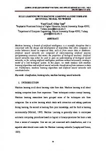
3.2. Agglomerative Hierarchical Clustering (AHC) Starting with all n objects to be clustered, AHC groups these objects into successively fewer than n sets. It is a hierarchical nonoverlapping method that specify a sequence P0 , ..., Pw of partitions of the objects in which P0 is the disjoint partition, Pw is the conjoint partition, and Pi is a refinement (in the usual sense) of Pj for all 0 ≤ i < j ≤ w. It is a sequential method since the same algorithm is used iteratively to generate Pi+1 from Pi for all 0 ≤ i < w. Is is a pair-group method: at each iteration exactly two clusters are agglomerated into a single cluster [20]. Although it is more suitable to find many clusters through this unsupervised approach, in this experiment we used Agglomerative Hierarchical Clustering (AHC) to find two clusters (AHC experiment), i.e., our result is the two main subgroups obtained from the whole datasets (the smaller subgroups are irrelevant for this experiment). The resulting Agglomerative Hierarchical Clustering with the two clusters found is represented in Figure 1 with all possible three dimensional representations, i.e., three morphological parameters combined at time to build the 3D data space.
True label
S E
Pred. label S E 946 48 175 793
Table 4: Confusion Matrix for the experiment with Agglomerative Hierarchical Clustering.
doi:10.6062/jcis.2016.07.03.0114
Discussion Paper
Barchi et al.
Figure 1: Reprentations in three dimensions of the result of Agglomerative Hierarchical Clustering.
5
doi:10.6062/jcis.2016.07.03.0114
Discussion Paper
Barchi et al.
6
4. Concluding Remarks The Tables 5 and 6 present a comparative summary of the supervised and unsupervised experiments, respectively, with precision P (T P/(T P + F P )) and recall R (T P/(T P + F N )) for each galaxy class: spiral (S) and elliptical (E). F-score (F1 = 2 × (P × C)/(P + C)), Overall Accuracy (OA = (T P + T N )/(T P + T N + F P + F N )) and Kappa index (κ) for each experiment also appear in these tables. Kappa is a statistic which measures inter-rater agreement for classification problems. Inter-rater agreement, also known as concordance, is the degree of agreement among raters. Thus, Kappa measures the degree of agreement beyond what would be expected by chance alone. This measure has a maximum value of 1, where 1 represents total agreement; and values close to and below 0, indicate no agreement, or agreement was exactly the one expected by chance. #Exp SVM1 SVM2 SVM3 SVM4 DT1 DT2 DT3 DT4
P(S) % 98.556 98.601 98.748 98.818 98.863 98.85 98.682 98.758
R(S) % 98.684 98.49 98.454 98.532 98.792 98.707 98.673 98.703
P(E) % 82.767 80.631 79.6 80.06 83.586 82.738 82.416 83.213
R(E) % 81.383 81.805 82.864 83.333 84.404 84.37 82.513 83.819
F1 % 0.9862 0.9855 0.9860 0.9867 0.9883 0.9866 0.9868 0.9873
OA % 97.437 97.3 97.395 97.528 97.815 97.726 97.541 97.643
κ 0.807 0.798 0.798 0.803 0.828 0.823 0.811 0.822
Table 5: Precision (P), Recall (R) and F-score (F1 ) for each class; Overall Accuracy (OA) and κ for each supervised experiment. #Exp K-means1 K-means2 AHC
P(S) % 85,847 85,847 95,171
R(S) % 95,953 95,953 84,389
P(E) % 93,662 93,662 81,921
R(E) % 87,172 87,172 94,293
F1 % 0.8926 0.8926 0.8946
OA % 89,806 89,806 88,634
κ 0,796 0,796 0,772
Table 6: Precision (P), Recall (R) and F-score (F1 ) for each class; Overall Accuracy (OA) and κ for each unsupervised experiment. In general, DTs have the best results, considering CN as the most important feature to separate galaxies into spiral and elliptical (responsible attribute for the first decision in all DTs). The Grid Search applied in the supervised methods optimized the OA. Due to the unbalance in the dataset (44760 galaxies labeled as S and 3385 as E), none experiment reached Kappa index (κ) of 0,9, although the interval 0, 8 ≤ κ ≤ 1 is considered of excellent concordance. The recall was also affected by this unbalance. However, all supervised methods have over 97% of OA. For future works with clustering methods, we plan to build trainned models with this dataset to give supervision in this classification task with bigger unlabeled datasets. Also, we are studying to apply Generative Adversarial Networks (GAN) [21] and other Deep Learning techniques to improve galaxy morphology with machine learning further. Acknowledgments. PB, RS, RRR and RRdC thank CAPES, CNPq and FAPESP for partial financial support. RRdC acknowledges financial support from FAPESP through a grant # 2014/11156-4.
References [1] Al-Jarrah, O. Y., Yoo, P. D., Muhaidat, S., Karagiannidis, G. K. & Taha, K. (2015). Efficient machine learning for big data: A review. Big Data Research, 2 (3), 87-93.
doi:10.6062/jcis.2016.07.03.0114
Discussion Paper
Barchi et al.
7
[2] Srivastava, A. N. (Ed.). (2012). Advances in machine learning and data mining for astronomy. Chapman and Hall/CRC. ˇ Connolly, A. J., VanderPlas, J. T. & Gray, A. (2014). Statistics, Data Mining, and Machine [3] Ivezi´c, Z., Learning in Astronomy: A Practical Python Guide for the Analysis of Data. Princeton University Press. [4] Feigelson, E. D., & Babu, J. (Eds.). (2006). Statistical challenges in astronomy. Springer Science & Business Media. [5] Zaane, O. R. (1999). Introduction to data mining. [6] de Carvalho, R. R., & Rosa, R. R. (2014). What Drives the Stellar Mass Growth of Early-Type Galaxies? Born or made: the saga continues... [7] de Carvalho, R. R. & Rosa, R. R. (2016). Sistema Computacional Baseado em Novas Tecnologias de Alto Desempenho para Anlise Morfomtrica Intensiva em Imagens Digitais. [8] Ferrari, F., de Carvalho, R. R., & Trevisan, M. (2015). Morfometryka A new way of estabilishing morphological classification of galaxies. The Astrophysical Journal, 814 (1), 55. [9] Andrade, A. P. A., Ribeiro, A. L. B., & Rosa, R. R. (2006). Gradient pattern analysis of cosmic structure formation: Norm and phase statistics. Physica D: Nonlinear Phenomena, 223 (2), 139-145. [10] Sautter, Rubens, et al. (2017). In preparation [11] Willett, K. W., Lintott, C. J., Bamford, S. P., Masters, K. L., Simmons, B. D., Casteels, K. R., ... & Melvin, T. (2013). Galaxy Zoo 2: detailed morphological classifications for 304 122 galaxies from the Sloan Digital Sky Survey. Monthly Notices of the Royal Astronomical Society, stt1458. [12] Ball, N. M., & Brunner, R. J. (2010). Data mining and machine learning in astronomy. International Journal of Modern Physics D, 19 (07), 1049-1106. [13] Vasconcellos, E. C., De Carvalho, R. R., Gal, R. R., LaBarbera, F. L., Capelato, H. V., Velho, H. F. C., ... & Ruiz, R. S. R. (2011). Decision tree classifiers for star/galaxy separation. The Astronomical Journal, 141 (6), 189. [14] Schawinski, K., Zhang, C., Zhang, H., Fowler, L., & Santhanam, G. K. (2017). Generative Adversarial Networks recover features in astrophysical images of galaxies beyond the deconvolution limit. arXiv preprint arXiv:1702.00403. [15] Pedregosa, F., Varoquaux, G., Gramfort, A., Michel, V., Thirion, B., Grisel, O., ... & Vanderplas, J. (2011). Scikit-learn: Machine learning in Python. Journal of Machine Learning Research, 12 (Oct), 2825-2830. [16] Hearst, M. A., Dumais, S. T., Osuna, E., Platt, J., & Scholkopf, B. (1998). Support vector machines. IEEE Intelligent Systems and their Applications, 13 (4), 18-28. [17] Cortes, C., & Vapnik, V. (1995). Support-vector networks. Machine learning, 20 (3), 273-297. [18] Quinlan, J. R. (1986). Induction of decision trees. Machine learning. 1 (1), 81-106. [19] Hartigan, J. A., & Wong, M. A. (1979). Algorithm AS 136: A k-means clustering algorithm. Journal of the Royal Statistical Society. Series C (Applied Statistics), 28 (1), 100-108. [20] Day, W. H., & Edelsbrunner, H. (1984). Efficient algorithms for agglomerative hierarchical clustering methods. Journal of classification, 1 (1), 7-24. [21] Goodfellow, I., Pouget-Abadie, J., Mirza, M., Xu, B., Warde-Farley, D., Ozair, S., ... & Bengio, Y. (2014). Generative adversarial nets. In Advances in neural information processing systems (pp. 26722680).