Improving Inversion Median Computation using Commuting Reversals and Cycle Information⋆ William Arndt and Jijun Tang Department of Computer Science and Engineering University of South Carolina Columbia, SC 29208, USA
Abstract. In the past decade, genome rearrangements have attracted increasing attention from both biologists and computer scientists as a new type of data for phylogenetic analysis. Methods for reconstructing phylogeny from genome rearrangements include distance-based methods, MCMC methods and direct optimization methods. The latter, pioneered by Sankoff and extended with the software suite GRAPPA and MGR, is the most accurate approach, but is very limited due to the difficulty of its scoring procedure–it must solve multiple instances of median problem to compute the score of a given tree. The median problem is known to be NP-hard and all existing solvers are extremely slow when the genomes are distant. In this paper, we present a new inversion median heuristic for unichromisomal genomes. The new method works by applying sets of reversals in a batch where all such reversals both commute and do not break the cycle of any other. Our testing using simulated datasets shows that this method is much faster than the leading solver for difficult datasets with only a slight accuracy penalty, yet retains better accuracy than other heuristics with comparable speed. This new method will dramatically increase the speed of current direct optimization methods and enables us to extend the range of their applicability to organellar and small nuclear genomes with more than 50 inversions along each edge. As a further improvement, this new method can very quickly produce reasonable solutions to problems with hundreds of genes.
1 Introduction Because of the advent of high-throughput sequencing and the consequent reduction in costs, we are seeing an explosion in the amount of genomic data of all types. In particular, the availability of fully sequenced and well annotated genomes allows us to move beyond the mere sequence level in the study of genomic evolution. Once a genome has been annotated to the point where gene homologs can be identified, each gene family can be assigned a unique integer and each chromosome represented by an ordering (a permutation) of signed integers, where the sign indicates the strand. Rearrangement of genes under inversion, transposition, and other operations such as duplications, deletions and insertions, then amount to rearrangements of these orderings. Such rearrangements are known to be an important evolutionary mechanism [11] ⋆
Contact author: Jijun Tang,
[email protected]
2
and their use in reconstructing phylogenies has been studied intensely since the pioneering papers of Sankoff [5, 24]. Biologists have embraced this new source of data in their phylogenetic work [11, 19, 22] and also in comparative genomics [21], while computer scientists are slowly solving the difficult problems posed by the manipulations of these gene orders [18]. During the past several years, computer scientists have been able to make substantial progress in genome rearrangement research: with the solution for inversion distance [13] and inversion median [10], we were able to estimate phylogenies and ancestral genomes based on inversions (the dominant events in organellar genomes). There are several widely used methods for genome rearrangement analysis, including neighbor-joining [23], GRAPPA [17], MGR [7] and Badger [15]. Using the later three generally will achieve better accuracy than using distance based methods such as neighbor-joining. The main software packages for reconstructing the inversion (or breakpoint) phylogeny are GRAPPA and MGR. Their basic optimization tool is an algorithm for computing the inversion (or breakpoint) median of three genomes. However, using GRAPPA and MGR to analyze organismal genomes with many events is extremely expensive, because the median computation takes time exponential in both the size of the genomes and the distances among genomes. In this paper, we present a fast yet accurate heuristic using commuting reversals to improve the inversion median computation for both distant and large genomes. We will also provide some discussions regarding inversion medians when the number of events approach saturation.
2 Backgrounds 2.1
Genome Rearrangements
We assume a reference set of n genes {g1 , g2 , · · · , gn }, thus a unichromisomal genome can be represented as a signed ordering of these genes, and each gene is given an orientation that is either positive, written gi , or negative, written −gi . Genomes can evolve through events including inversions, transpositions and transversions. Let G be the genome with signed ordering of g1 , g2 , · · · , gn . An inversion between indices i and j (i ≤ j), transforms G to a new genome with linear ordering g1 , g2 , · · · , gi−1 , −g j , −g j−1 , · · · , −gi , g j+1 , · · · , gn A transposition on genome G acts on three indices i, j, k, with i ≤ j and k ∈ / [i, j], picking up the interval gi , gi+1 , · · · , g j and inserting it immediately after gk . Thus genome G is replaced by (assume k > j): g1 , · · · , gi−1 , g j+1 , · · · , gk , gi , gi+1 , · · · , g j , gk+1 , · · · , gn An transversion is a transposition followed by an inversion of the transposed subsequence; it is also called an inverted transposition. 2.2
Distance Computation
Given two genomes G1 and G2 , we define the edit distance d(G1 , G2 ) as the minimum number of events required to transform one genome into the other. The breakpoint distance [24] is not a direct evolutionary distance measurement. A breakpoint in G1 is
3
defined as an ordered pair of genes (gi , g j ) such that gi and g j is adjacent in G1 but not in G2 . The breakpoint distance is simply the number of breakpoints in G1 relative to G2 . When only inversions are allowed, the edit distance is the inversion distance. Hannenhalli and Pevzner [13] developed a mathematical and computational framework for signed gene-orders and provided a polynomial-time algorithm to compute the edit distance between two signed gene-orders under inversions; Bader et al. [1] later showed that this edit distance can be computed in linear time. However, computing the inversion distance is NP-hard in the unsigned case [9]. The HP algorithm is based on the breakpoint graph (Fig 1). We assume without loss of generality that one permutation is the identity. We represent gene i by two vertices, −i and +i, connected by an edge. The edge is oriented from +i to −i when gene i is positive, but oriented in the reverse direction when it is negative. Two additional vertices 0 and n + 1 are also added. These vertices can be connected with two sets of edges, one for each genome. One set of edges, called desire edges, represent the identity genome and is shown with dashed arcs in Fig 1. The other edges represent the current state of the genome and are shown with solid lines; these are called reality edges. In both set of edges, 0 always connects to −1 and n + 1 always connects to +n. The crucial concept is that of alternating cycles in this graph, i.e., cycles of even length in which every odd edge is a desire edge and every even one is a reality edge. Overlapping cycles in certain configurations create structures known as hurdles, and a very unlikely configuration of such hurdles can form a single fortress (please refer [13] for details). Hannenhalli and Pevzner [13] proved that the inversion distance between two signed permutations of n genes is given by n − #cycles + #hurdles + (1 i f f ortress present, 0 otherwise)
−2 0
+2
4 −2
−4
3 +4
−3
−1 +3
+1
−1
5
Fig. 1. Breakpoint graph between genome (-2 4 3 -1) and the identity genome (1 2 3 4).
2.3
Sorting and Commuting Reversals
Almost all the distance computation methods return one (and only one) minimum sorting sequence. Siepel [26] extended the HP theorem to find all sorting reversals, i.e., all possible inversions that appear as the first step in the sorting. Fig 2 gives one example of sorting reversals: there are eight possible inversions that bring G2 one step closer to G1 (the identity genome). This algorithm can be easily extended to enumerate all minimum sorting sequences by identifying every sorting reversals at each step of the sorting.
4
G2 : −1 1
−2
−3
−4
−5
2
3
4
5
G1 : 1
6
2
3
4
5
indicates start and end points of a reversal
7 8
Fig. 2. Eight sorting reversals that bring (-1 -2 -3 -4 -5) one step closer to (1 2 3 4 5).
The concept of commuting reversals was introduced in [6] where the context was sorting between two permutations using inversions. Two different sorting inversions acting on the same permutation are defined to commute as follows: separate the permutation integers into three sets: those integers which are only members of the first inversion, those which are only members of the second, and those which are members of both. The two sorting inversions commute if and only if one of these three sets is empty. Commuting inversions have a desirable property that applying them to a permutation will always obtain the same result no matter the order they are applied.
1
2
3
4
5
6
1 2 3 4 5 6
A
A B
(a) set only affected by A: [2, 3] set only affected by B: [4, 5] set affected by A ∩ B: φ
B (b) set only affected by A: [5] set only affected by B: φ set affected by A ∩ B: [2, 3, 4]
1 2 3 4 5 6 A B (c) set only affected by A: [2] set only affected by B: [5] set affected by A ∩ B: [3, 4]
Fig. 3. Examples of commuting inversions (a and b) and non-commuting inversion (c).
2.4
Inversion Median Problem
Given three genomes (permutations) π1 , π2 , π3 and another genome π0 , we define the median score from π0 as d(π0 , π1 ) + d(π0 , π2 ) + d(π0 , π3 ). The median problem on three genomes is to find genome π0 that minimizes the median score between itself and each of the three given genomes π1 , π2 , π3 . We also define the perfect median score as l m d(π1 ,π2 )+d(π1 ,π3 )+d(π2 ,π3 ) , which is the lower bound of the score for a median problem. 2 The median problem is NP-hard [8, 20] even for simple distance definition such as breakpoint distance. Seeking a median that minimizes the breakpoint distance can be transformed into a special instance of the well-studied Traveling Salesperson Problem [4], hence can be solved relatively efficiently. But in practice, the breakpoint median is not effective—it is easy to obtain trivial solutions (where the median gene-order coincides with one of the leaves), hence is not as accurate as using inversion median for genome rearrangement analysis [16].
5
The inversion median problem is to find a median genome that minimizes the sum of inversion distances on the three edges. Four inversion median solvers have been proposed. Caprara’s solver [10] is based on an extension of the breakpoint graph, while that developed by Siepel and Moret [25] runs a direct search. Both Caprara’s and Siepel’s median solvers are exact and are included in GRAPPA. In practice, Caprara’s median solver is faster when the genomes are not close. Both MGR [7] and rEvoluzer [2] are heuristics, using similar approach: they both seek good reversals that bring a genome closer to the ancestral genome. For three genomes, the MGR algorithm evaluates all possible inversions for each of the three genomes, identifying good reversals that bring a genome closer to the ancestral genome. Since the ancestral genome is unknown, the algorithm chooses inversions which make G1 closer to both G2 and G3 as good reversals. Thus the algorithm will iteratively carry on good reversals in the three genomes until all three are transformed into an identical genome, which is viewed as the most likely ancestral median. rEvoluzer improves the MGR procedure by selecting inversions that cannot destroy any conserved intervals. Although rEvoluzer achieves some speedup over GRAPPA, like MGR, the median gene orders it obtained is not as good as those returned by GRAPPA [2]. All these median solvers become extremely slow for large and distant genomes. A common speedup process used by all methods makes use of the concept of conserved adjacency. A gene pair (x, y) is conserved adjacent if (x, y) or its inverse (−y, −x) is present in all genomes as consecutive elements [14]. A block of k adjacent genes can be replaced by a new gene and the total number of genes reduces by k − 1 [7]. This condensation procedure is very effective when the genomes are close: a median of genomes with 1, 000 genes and 50 inversions per edge can be condensed to ∼ 200 genes only. In practice, given the smallest edge length e and number of genes n, we found the ratio ne is a good indicator about the difficulty of inversion median problem. Siepel’s median solver cannot handle datasets with ne > 15%, and its search approach limits it to small genomes (< 100 genes) as well. On the other hand, Caprara’s median solver will be able to handle datasets with 1, 000 genes for ne ≤ 20%.
3 Inversion Median Computation using Commuting Reversals We set out to improve the speed of inversion median computation with the goal that the new median solver should have accuracy that is comparable to Caprara’s median solver. The new algorithm is different from MGR and rEvoluzer in that it will conduct a direct search from one of the known genomes, using sorting reversals to limit the search space. Our algorithm also improves over Siepel’s method by using commuting reversals in the set of sorting reversals from the start genome to both of the other two genomes. Our new median solver will also report multiple solutions, a property lacking in almost all existing methods. 3.1
A Naive Approach
Let us first present a naive approach. Suppose the three input permutations are π1 , π2 , and π3 , and assume all median scores are with respect to π1 , π2 , and π3 . Define a
6
recursive function which has input π1 , π2 , π3 , and π4 , where π4 is set as π1 when the function is first called. In this function first obtain two sets of sorting reversals, set α which contains sorting reversals from π4 to π2 , and set β which contains sorting reversals from π4 to π3 . Let set γ be the intersection of α and β. Repeat the following process until γ is empty: remove one inversion from γ and apply to π4 to obtain π′4 , determine the median score of π′4 and compare to the lowest median score seen so far in the search. If the median score of π′4 is less than or equal to the best-so-far, report the score and π′4 . Call the recursive function with arguments π1 , π2 , π3 , and π′4 . Several concerns make this method undesirable. Primarily, the amount of computation required increases exponentially with both the number of inversions separating the three permutations and the number of genes in each genome. Second, it can be shown by exhaustively searching permutations against a small inversion median problem, that a median permutation does not necessarily lie on a sorting path between two of the three initial permutations; thus the presented naive approach cannot guarantee an optimal solution because some and possibly all paths to medians would require that one or more reversals which are not members of γ be chosen. We will not attempt to improve this aspect of the naive method as doing so would require a large number of additional inversions be considered in set γ with very little return on the massive amount of new computation being performed. The biggest problem of the naive approach is that it performs a large amount of redundant computation by visiting the same permutation multiple times. This can be reduced by using information about commuting reversals. Imagine a set of sorting reversals which sort π1 towards both π2 and π3 . Select any pair of these reversals A and B which occur along the path to a median. if reversals A and B do not commute, then changing the order that A and B are applied affects the resulting permutation (Fig 3c); if A and B commute (Fig 3a and Fig 3b) then the naive method will search the same permutation at least twice, since both choices of ordering the application of A and B result in the same permutation. 3.2
An Improved Algorithm
The above analysis leads to a method to speed up the search by removing a large portion of this redundancy. Obtain from the set γ reversals with the additional property that all pairs of inversions commute. This allows the order of applying these reversals to be ignored; every permutation which can be reached by applying any number of these commuting reversals can be enumerated and scored one time instead of enumerating permutations by the paths which lead to them. If n is the number of commuting reversals, then 2n permutations can be reached, but the total number of paths to these permutations is O(nn ). Which set of the 2n permutations should be chosen? We have experimented with several methods: – Brute force method which scores every 2n permutation and chooses the best median score π′4 , with good results but an obvious time complexity drawback. – A method which draws samples from the 2n permutations and chooses the best median score among them. This approach reduces both the time required and the
7
accuracy; in general the quality of the results are proportional to the fraction of the space being searched. – The simplest method of all, and surprisingly effective, is to apply all reversals in the set, i.e., obtaining π′4 from by applying all non-interfering reversals to π4 . The quality of this method depends on the ratio of the size of the permutation to the size of the reversal set. This approach works well until the ne ratio is 30 − 40%. Beyond that point each search step normally increases the median score and tends to converge with worse results than a trivial solution. The previous example, where applying all commuting reversals results in a worse median score, demonstrates there is a more complex interaction between the application of a single sorting reversal to a permutation and its influence on other sorting reversals. This interference between sorting reversals comes from the breaking of cycles in the breakpoint graphs of the problem instance. Imagine a breakpoint graph with one cycle containing two sorting reversals that commute. Applying either of those sorting reversals will alter the breakpoint graph to create two cycles. Afterwards, two possibilities exist: either both of the reality edges of the second reversal will remain in the same cycle, in which case this reversal will be a sorting reversal, or the reality edges of the second reversal will be separated into different cycles, in which case it will no longer be a sorting reversal. This line of thought leads to a concept similar to commuting reversals, only transferred to breakpoint graph cycle interactions. 3.3
Parallel and Perpendicular Sorting Reversals
We call a pair of sorting reversals parallel on a single breakpoint graph if they commute, break reality edges in the same cycle of the breakpoint graph, and applying both inversions to the permutation creates two additional cycles. On the other hand, a pair of sorting reversals are perpendicular on a single breakpoint graph if they commute, break reality edges in the same cycle of the breakpoint graph, and applying both inversions to the permutation creates one additional cycle. When multiple breakpoint graphs present, we also call a pair of reversals parallel if in all such graphs the reality permutation is the same (the generalization that the desire permutation is the identity is relaxed), both inversions sort each graph, and the inversions are not perpendicular on any of the considered graphs. A pair of reversals are perpendicular over multiple breakpoint graphs if in all such graphs the reality permutation is the same, the inversions sort each graph, and the inversions are perpendicular on any of the graphs. Theorem 1. Consider the breakpoint graph from π4 to π2 , the breakpoint graph from π4 to π3 and the set of commuting sorting inversions γ. Inversions can be removed from the set until no two inversions are perpendicular over both graphs, and the result is a set of sorting inversions which when applied to π4 in any order improve its median score by an amount equal to the number of inversions which remain in γ. Proof. Given set γ contains inversions which sort π4 towards both π2 and π3 , that no pair of these inversions are perpendicular, and that all pairs of inversions commute. We prove the theorem by induction. As the inductive step, repeatedly remove any inversion from
8
γ and apply it to π4 . No pair of inversions in γ are perpendicular, so no previous choice was possible which will affect the sorting property of the current inversion. The chosen inversion is a sorting inversion to both targets, so d(π4 , π1 ) will increase by 1, d(π4 , π2 ) and d(π4 , π3 ) will both decrease by 1. During one inductive step the median score will improve by 1 and the cardinality of γ will lower by one. In the base case, set γ is empty and there are no additional inversions which will sort π4 towards both π2 and π3 . Fig 4 describes a simple graph method to visualize the parallel and perpendicular inversion properties. We first obtain the set of sorting inversions between two permutations, but additionally save the cycle membership and order in which each reality edge appears when transversing a cycle. For each cycle, in a ring, draw a break location node for each reality edge in the breakpoint graph and label the node with the genes that appear on each side of the edge, and draw an edge representing the desire edge to both of its neighbors. For each sorting reversal which acts on two reality edges in the same cycle (not inversions which merge hurdles or cut a hurdle or fortress), draw a cut chord connecting both of the corresponding break location nodes in the ring. This chord corresponds to the cut that divides the cycle into two smaller cycles when the inversion is applied, and shows which break location nodes will remain in the same cycle and which will be separated. For every pair of inversions in the same cycle, if the cut chord for each intersect, then this pair of inversions is perpendicular, otherwise, the inversions are parallel.
−3 2
4
−1 a
−2
−3
−4
−5
b
c
d
e
0
−5
c
b
−1
e
a
6
d
f
f
1
5 −2
−4 3
Fig. 4. Graph representation of cycle interferences on a set of commuting reversals, genes 0 and 6 represent linear chromosome endpoints
A special case exists where two inversions share a break location node, as sometimes such inversions will be parallel and sometimes perpendicular. The problem is that when an inversion is applied it separates the two genes labeling a break location node and puts one in each of the newly formed cycles, but different inversions make this decision in different ways, depending on the layout of the permutation. We address this issue in the implementation by treating any inversions which share a break location as perpendicular, with the drawback of sometimes removing inversions from γ which do not actually need to be removed.
9
3.4
The Final Algorithm
The overall heuristic of our new unichromosomal median solver is presented in Fig 5. Several details worth mentioning. First, the choice of the start permutation has some impact and our experiments show that using the permutation nearest to the center produces the best median scores. Second, despite our efforts to prevent redundant computation, a very large amount still occurs and we used a permutation hash table to check for redundant search paths. This is not a critical aspect and can be removed with little impact–in fact, due to memory constraints it must be removed for genomes larger than approximately 400 genes. The last to mention is the use of set ∆. This is inherited from the naive method as a way to allow every sorting reversal at least one chance to be searched. We will continue to investigate better ways of directing the search past the initial steps. InversionMedianSolver: input permutations π1 , π2 , π3 Compute the pairwise inversion distances between π1 , π2 , π3 Choose the one with the smallest sum of its two distances as π4 If π1 was not assigned to π4 , swap it with the permutation which was Initilize a global variable BestSoFar to an arbitrarily large value Call RecursiveSearch: π1 , π2 , π3 , π4 RecursiveSearch: input permutations π1 , π2 , π3 , π4 Obtain set α of sorting inversions from π4 , π2 Obtain set β of sorting inversions from π4 , π3 Obtain set γ, the intersection of α and β Call UseGamma: γ, π1 , π2 , π3 , π4 While set ∆ contains elements: Set γ to ∆ and clear ∆ Call UseGamma: γ, π1 , π2 , π3 , π4 UseGamma: input set γ and permutations π1 , π2 , π3 , π4 , output set ∆ For each pair of inversions in γ: If inversions do not commute add 1 weight to each; Repeat until the weight of all inversions in γ is 0: Find the inversion A with largest weight Remove A from γ and place in set ∆ Reduce weight of each inversion not commute with A by 1 For each pair of inversions in γ: If pair is perpendicular, add 1 weight to each Repeat until the weight of all inversions in γ is 0: Find the inversion A with largest weight and remove A from γ Reduce weight of each inversion perpendicular to A by 1 Apply the reversals in set γ to π4 to create π′4 Calculate the median score of π′4 with respect to π1 , π2 , π3 If the score is less than or equal to BestSoFar Assign the score to BestSoFar and output π′4 If the median score of π′4 is less than the score of π4 Call RecursiveSearch: π1 , π2 , π3 , π4 Fig. 5. Algorithm overview for the new inversion median solver.
10
4 Experimental Results 4.1
Setup of Simulations
We set out to examine the performance (in terms of speed and accuracy) of the new method, using simulated datasets. Because all existing median solvers have very good performance when genomes are close, we only test distant genomes and compare our method against Caprara’s solver (slower but exact), and MGR (faster but less accurate). We focused our experiments on organelle genomes and generated datasets of three genomes with 100 genes for each genome (larger genome sizes were also tested). We first generated trees with three leaves and one internal node, assigned the identity permutation on the internal node and generate the three leaves by applying rearrangement events along each edge respectively. The number of events on each edge is governed by two parameters: the number of overall evolutionary events and the tree shape. We used various number of evolutionary rates: letting r denote the total number of events along all three edges, we used values of r in the range of 80 to 140. We found from our experience that the tree shape plays an important role in median computation, thus we used three tree shapes for each r: a tree with almost equal length edges, i.e., the ratio of three edges are (1 : 1 : 1); a tree with one edge a bit longer than the other two, i.e., of ratio (2 : 1 : 1); a tree with on edge much longer than the other two, i.e., of ratio (3 : 1 : 1). While all computations were based on inversion distances and inversion medians, we generated the data with a deliberate model mismatch to test the robustness of the methods, using a mix of 80% inversions and 20% transpositions. For each combination of parameter settings, we ran 10 datasets and averaged the results. Experiments were conducted on a Linux cluster with 152 Intel Xeon CPUs, but each CPU works independently on a test task. MGR command line options -c -H1 were used. 4.2
Accuracy
Caprara’s median solver had no problem to finish all datasets with evolutionary rate r = 80 and r = 100; however, it could finish a very small number of datasets for r = 120 and 140: only four out of 60 datasets finished within 48 hours of computation. Here we report the result separately using slightly different criteria for r ≤ 100 and r ≥ 120. For r ≤ 100, we report the average median score from our method, Caprara’s solver, and MGR. We also report the average perfect (lower bound) median score, which is the best possible score for any median solver. Table 1 shows the result, which indicates that our method is very accurate, with < 1.5% errors. Our method is most accurate when all three edges are almost equal length, with 70% datasets report median score to those found by Caprara’s, while the other 30% are only one score away. For r ≥ 120, since Caprara’s solver cannot finish all datasets, we only report the average median score from our method and compare it to MGR and the average perfect median score. Table 2 shows the result, which indicates that our method can find better medians than MGR does. An additional measure of the quality of results is the distance to the simulated ancestor genome. Here we report the average distance to the ancestor for the three methods for those Caprara’s method could complete in Table 3, and in Table 4 those sets which Caprara’s method could not solve.
11 (1:1:1) (2:1:1) r=80 r=100 r=80 r=100 Prefect median score 86.2 104.2 89.4 105.8 Caprara’s median score 87.9 107.6 91.4 109.8 New method’s median score 88.2 109.5 91.8 111.4 MGR median score 90.3 113.7 94.3 116.8 Table 1. Comparison of median scores for r ≤ 100.
(3:1:1) r=80 r=100 85.7 101.3 88.0 105.2 89.1 106.7 89.8 110
(1:1:1) (2:1:1) r=120 r=140 r=120 r=140 Prefect median score 116.1 123.5 116.1 122.7 New method’s median score 125.8 135.3 124.5 134.7 MGR median score 132.9 143.6 131.4 142.8 Table 2. Comparison of median scores for r ≥ 120.
(3:1:1) r=120 r=140 110.3 117.6 117.9 127.0 123.6 135.1
(1:1:1) (2:1:1) (3:1:1) r=80 r=100 r=80 r=100 r=80 r=100 Caprara’s method 4.5 18.2 7.2 16.8 5.2 15.7 New Method 9.3 21.7 9.6 20.4 7.2 18.2 MGR 9.3 23.5 11 25.4 9.1 18.6 Table 3. Comparison of distance to simulated ancestor for r ≤ 100.
(1:1:1) (2:1:1) (3:1:1) r=120 r=140 r=120 r=140 r=120 r=140 New method 39.8 49.3 35.2 45.4 23.1 32.1 MGR 40.7 51.6 37.5 49.5 29.7 37.7 Table 4. Comparison of distance to simulated ancestor for r ≥ 120.
4.3
Speed
We recorded the running time for each run as well. Since our method will report all results it can find, there are two measures: 1) the time it finds the first result, and 2) the average number of results it finds within the limit of one hour. Table 5 and Table 6 shows the first time comparison. When the datasets are relatively easy (r = 80), Caprara’s solver is much faster than our method. However, it slows down very quickly when the difficulty increases, and almost no dataset can be finished for r ≥ 120. Meanwhile, the running time of our method is quite consistent with fewer than 30 minutes were used even for the most difficult datasets, which is comparable to the speed of MGR. In general, our method found 12 medians with the same score within one hour. However, the number is not consistent: some datasets have only one result, while others have as many as 120 results. Additionally, by checking inversions on the found medians
12 (1:1:1) (2:1:1) (3:1:1) r=80 r=100 r=80 r=100 r=80 r=100 New method’s time 324 551 123 409 1.6 9.3 MGR time 11.2 51.9 11.6 78.2 10.3 35 Caprara’s time 3.6 12876 57.2 31387 4.3 6908 Table 5. Comparison of running time for r ≤ 100 (in seconds).
(1:1:1) (2:1:1) (3:1:1) r=120 r=140 r=120 r=140 r=120 r=140 New method’s time 1485 1187 673 453 30 226 MGR time 271.6 560.1 237.8 626.9 135.3 385.4 Caprara’s time > 172880 > 172880 > 172880 > 172880 > 172880 > 172880 Table 6. Comparison of running time for r ≥ 120 (in seconds).
which do not change the median score, on average for each found median two more can be quickly located, though they are not significantly different from those already found. Table 7 shows the average number of medians found by our method.
r=80 r=100 r=120 r=140 (1:1:1) 27.4 4.0 29.9 7.1 (2:1:1) 11.6 22.9 13.8 8.9 (3:1:1) 6.0 9.1 5.6 11.4 Table 7. Average number of medians found for each test case.
4.4
Medians of Larger Genomes
We tested the performance of our new method on some simulated datasets of larger genomes. The simulations were created with the same parameters, except the number of genes was increased to 500. The tested trees all have edge lengths of 100, 100, and 200, producing a tree with ne = 20%. Neither Caprara’s solver nor MGR could produce results for any of these trees. Our method, however, can consistently return medians which are within 7% of the lower bound in less than 30 seconds.
5 Discussion The method presented here offers acceptable solutions for the median problem which previous methods are either completely unable to solve in a timely manner, or less accurate. The source of speedup is that our search complexity increases not directly with the
13
number of genes and events, but with the size of the set of sorting reversals which sort one input permutation towards both of the others. The two types of problems which our method performs relatively poorly are those with a small number of events, which limit the set of shared reversals causing the search to be too shallow, and problems that have all three edges of approximately equal length causing the shared sorting reversal set to be too large resulting in an overly broad search. Real world problems, however, can either be limited to small data sets, in which case existing tools are well sufficient, or may require consideration of large genomes of which such genomes are rarely symmetrical, making our method appropriate. We believe there is a big problem in the general approach of using the inversion median problem to solve phylogenetic trees composed of distant genomes, a topic discussed in detail in [12]. The direct optimization methods (GRAPPA and MGR) are based upon minimizing the number of inversion events, which requires either the false assumption that there is only one optimal median solution for a given problem instance, or the slightly weaker assumption that although multiple optimal solutions exist, they are all equally valuable for construction of trees. The issue is most evident when viewing the distances between found medians and the true ancestor: although it is still proportional to median score, increasing the number of events causes the optimal median and ancestor genome to diverge. Several of our test simulations demonstrate the existence of multiple medians that form trees with edges differing by 30% or more, although the tree scores are equal. This shows instances of a median problem do not contain the amount of exact information which current tree methods presume they do. We do not believe that this cause is hopeless however, instead, the notion that any median with optimal score is an equal representative of an internal node should be replaced; new methods or tree building algorithms should be devised which use multiple medians as an intermediate step moving closer to the true ancestor. To obtain more accurate results for large genomes, we may need to find as many medians as possible and choose the one with the minimal total distance to all the others as the representative, or we may need to consider permutations with slightly less than optimal score if they appear in sufficiently large clusters. The structure of median problems has further vulnerabilities. We ran a small experiment where a random median problem of 10 genes was created, and the median score of every permutation (210 10!) in an exhaustive search was found. There are several findings from this experiment: 1) as confirmed by other researchers [3], there exist multiple medians–we found 81 medians for this experiment, with median score of 15; 2) Some of the medians were as far as 9 inversions from one another, but all these 81 medians gathered together in a cloud at the center of the problem space. In order to transverse from one of the initial permutations to a median, the choices of inversions remain very limited, and the possible paths remain very close, until the search nears where medians are located. If this general structure is similar to that of a large median problem instance, then this could be how using commuting reversals achieves its speedup, and additional methods to exploit this structure would likely exist.
14
6 Conclusions and Future Work In this paper we present a new inversion median solver using commuting reversals, and introduced the concept of parallel and perpendicular sorting reversals. We extensively tested the method and compare its performance with the leading median solver, using simulated datasets. The experimental results showed that our method is very accurate, and is much faster than the leading solver when the datasets are difficult. We will test the effectiveness of this median solver for phylogenetic reconstruction, and develop methods that can effectively use the multiple median solutions returned by our method to get closer to the true ancestor. We will also extend the concept of solving medians based on breakpoint cycle interactions. If care is taken when hurdles or a fortress are present, the visualization of breakpoint graph cycle interactions could be used to find an upper bound on sorting inversions by predicting and tracking the behavior as the number of cycles increases. This would proceed by examining which and how many potential reversals cut the cycles of other sorting inversions, and thus choose a inversion to apply which separates the break locations of least number of other possible sorting inversions.
7 Acknowledgments The authors were supported by US National Institutes of Health (NIH grant number R01 GM078991-01) and by the University of South Carolina. WA is also supported by a fellowship provided by Rothberg foundation. We also thank the anonymous reviewers for their comments and suggestions of improving the original draft.
References 1. Bader, D.A., B.M.E. Moret, and M. Yan (2001). A fast linear-time algorithm for inversion distance with an experimental comparison. J. Comput. Biol. 8(5), 483–491. 2. Bernt M., D. Merkle, and M. Middendorf (2006). Genome rearrangement based on reversals that preserve conserved intervals. IEEE/ACM Trans. on Comput. Biol. and Bioinfo. 3 (3), 275–288. 3. Bernt M., D. Merkle and M. Middendorf (2007). Using median sets for inferring phylogenetic trees. Bioinformatics 23 (2), 129-135. 4. Blanchette, M. and D. Sankoff (1997). The median problem for breakpoints in comparative genomics. In T, Jiang and D.T. Lee (Eds.), Proc. 3rd Comput. and Combin. Conf. (COCOON’97). Volume 1276 of Lecture Notes in Computer Science, 251–263. 5. Blanchette, M., G. Bourque, and D. Sankoff (1997). Breakpoint phylogenies. In S. Miyano and T. Takagi, eds., Genome Informatics, pages 25–34. Univ. Academy Press. 6. Bergeron, A., C. Chauve, T. Hartman and K. St-Onge (2002). On the Properties of Sequences of Reversals that Sort a Signed Permutation. Journal Ouvertes Biologie, Informatique, Mathematiques (JOBIM 2002), 99-108, 2002. 7. Bourque, G. and P. Pevzner (2002). Genome-scale evolution: Reconstructing gene orders in the ancestral species. Genome Research 12, 26–36. 8. Caprara, A. (1999). Formulations and hardness of multiple sorting by reversals. In Proc. 3rd Int’l Conf. on Comput. Mol. Biol. RECOMB99, 84–93. ACM Press. 9. Caprara, A. (1999) Sorting permutations by reversals and Eulerian cycle decompositions. SIAM J. Discrete Math. 12 (1), 91–110.
15 10. Caprara, A. (2001). On the practical solution of the reversal median problem. Proc. 1st Workshop on Algorithms in Bioinformatics (WABI’01), Volume 2149 of Lecture Notes in Computer Science, 238–251. 11. Downie, S. and J. Palmer (1992). Use of chloroplast DNA rearrangements in reconstructing plant phylogeny. In P. Soltis et al. (Eds.), Plant Molecular Systematics, 14–35. 12. Eriksen, N. (2007). Reversal and Transposition Medians. Theoretical Computer Sicence, 374, 111–126. 13. Hannenhalli, S. and P.A. Pevzner (1995). Transforming cabbage into turnip (polynomial algorithm for sorting signed permutations by reversals). Proc. 27th Ann. Symp. Theory of Computing STOC’95, 178–189, ACM Press. 14. Hannenhalli, S. and P.A. Pevzner (1996). To cut. . . or not to cut (applications of comparative physical maps in molecular evolution). Proc. 7th ACM-SIAM Symp. on Discrete Algorithms (SODA’96), 304–313, SIAM Press. 15. Larget, B., D.L. Simon, J.B. Kadane, and D. Sweet (2005). A Bayesian analysis of metazoan mitochondrial genome arrangements. Mol. Biol. and Evol., 22 (3), 486–95. 16. Moret, B.M.E., A. Siepel, J. Tang, and T. Liu (2002). Inversion medians outperform breakpoint medians in phylogeny reconstruction from gene-order data. Proc. 2nd Workshop on Algorithms in Bioinformatics (WABI’02), Volume 2452 of Lecture Notes in Computer Science, 521–536. 17. Moret, B.M.E., S. Wyman, D.A. Bader, T., Warnow, and M. Yan (2001). A new implementation and detailed study of breakpoint analysis. Proc. 6th Pacific Symp. on Biocomputing (PSB 01), World Scientific Pub., 583–594. 18. Moret, B.M.E., J. Tang, and T. Warnow (2005). Reconstructing phylogenies from genecontent and gene-order data. in Mathematics of Evolution and Phylogeny, O. Gascuel, ed., Oxford Univ. Press, 321–352. 19. Palmer, J. (1992). Chloroplast and mitochondria genome evolution in land plants. In R. Herrmann (Ed.), Cell Organelles, 99–133. 20. Pe’er, I. and R. Shamir (1998). The median problems for breakpoints are NP-complete. Elec. Colloq. on Comput. Complexity, 71. 21. Pevzner, P., and G. Tesler (2003). Human and mouse genomic sequences reveal extensive breakpoint reuse in mammalian evolution. Proc. of Natl. Acad. of Sci. USA, 100, 7672–7677. 22. Raubeson, L. and R. Jansen (1992). Chloroplast DNA evidence on the ancient evolutionary split in vascular land plants. Science 255, 1697–1699. 23. Saitou, N. and M. Nei (1987). The neighbor-joining method: A new method for reconstructing phylogenetic trees. Mol. Biol. Evol. 4, 406–425. 24. Sankoff, D. and M. Blanchette (1998). Multiple genome rearrangement and breakpoint phylogeny. J. Comput. Biol. 5, 555–570. 25. Siepel, A. and B.M.E. Moret (2001). Finding an optimal inversion median: experimental results. Proc. 1st Workshop on Algs. in Bioinformatics (WABI’01), Volume 2149 of Lecture Notes in Computer Science, 189–203. 26. Siepel, A. (2003). An algorithm to enumerate sorting reversals for signed permutations. J. Comput. Biol. 10, 575–597.