Improving Irrigation with Wetting Front Detectors - CiteSeerX

Improving Irrigation with Wetting Front Detectors

A report for the Rural Industries Research and Development Corporation by Richard Stirzaker, Richard Etherington, Ping Lu, Tony Thomson and Joyce Wilkie

February 2005 RIRDC Publication No 04/176 RIRDC Project No CSL-14A

© 2005 Rural Industries Research and Development Corporation. All rights reserved. ISBN 1 74151 085 6 ISSN 1440-6845 Improving Irrigation with Wetting Front Detectors Publication No. 04/176 Project No.CSL-14A The information contained in this publication is intended for general use to assist public knowledge and discussion and to help improve the development of sustainable industries. The information should not be relied upon for the purpose of a particular matter. Specialist and/or appropriate legal advice should be obtained before any action or decision is taken on the basis of any material in this document. The Commonwealth of Australia, Rural Industries Research and Development Corporation, the authors or contributors do not assume liability of any kind whatsoever resulting from any person's use or reliance upon the content of this document. This publication is copyright. However, RIRDC encourages wide dissemination of its research, providing the Corporation is clearly acknowledged. For any other enquiries concerning reproduction, contact the Publications Manager on phone 02 6272 3186.

Researcher Contact Details Richard Stirzaker CSIRO Land and Water PO Box 1666, ACT, 2601 Phone: Fax: Email:

(02) 6246 5570 (02) 6246 5965 [email protected]

In submitting this report, the researcher has agreed to RIRDC publishing this material in its edited form.

RIRDC Contact Details Rural Industries Research and Development Corporation Level 1, AMA House 42 Macquarie Street BARTON ACT 2600 PO Box 4776 KINGSTON ACT 2604 Phone: Fax: Email: Website:

02 6272 4819 02 6272 5877 [email protected]. http://www.rirdc.gov.au

Published in February 2005 Printed on environmentally friendly paper by Canprint

ii

Foreword Efficient use of water and nutrients are major issues for the irrigation industry and the science required to achieve these goals is relatively mature. However, most irrigation farmers do not measure the soil water status and very few monitor salt or nitrate. Under these conditions it is difficult to know how much progress is being made. This project introduced a Wetting Front Detector to farmers with the purpose of stimulating a rethink about irrigation management on-farm. The Wetting Front Detector was designed to be the simplest tool that could assist farmers to improve their understanding of water and salt movement in the soil. The experiences detailed in this report are drawn from work in orchards, vineyards and vegetable fields. The report shows that a simple tool can help irrigators to take another step along the difficult road of managing water and the solutes it contains. This project was funded from RIRDC Core Funds which are provided by the Australian Government. This report, an addition to RIRDC’s diverse range of over 1200 research publications, forms part of our Resilient Agriculture R&D program, which aims to develop systems that are compatible with environmental sustainability and deliver viable economic outcomes. Most of our publications are available for viewing, downloading or purchasing online through our website: • downloads at www.rirdc.gov.au/fullreports/index.html • purchases at www.rirdc.gov.au/eshop

Tony Byrne Acting Managing Director Rural Industries Research and Development Corporation

iii

Acknowledgments We thank the farmer collaborators who allowed us to install equipment on their properties (or the property they managed) and were prepared to field lots of questions particularly Joyce Wilkie and Michael Plane from Allsun farm, Gerry Clancy and David Haliday from Tatyoon and Ann and Haig Arthur and Martina Matzner from Acacia Hills, and Rob Giles and Rex Jaensch representing the Angas Bremer grape growers. Chapter 2 was co-authored with Joyce Wilkie from Allsun Farm and presented at the “Irrigation Association of Australia conference”, May 2002 in Sydney. Chapter 3 was co-authored with Joyce Wilkie and Sandeeren Sunassee from the Mauritius Agriculture Research and Extension Unit while working on a training program funded by the International Atomic Energy Association and will be presented at the Irrigation Association of Australia conference, May 2004 in Adelaide. Chapter 4 was co-authored with Richard Etherington from the NSW Agriculture and Chapter 5 with Dr Ping Lu from CSIRO Plant Industry in Darwin. Chapter 6 was co-authored with Tony Thompson from the Department of Water, Land and Biodiversity Conservation, South Australia. Additional funding from NSW Agriculture, CSIRO PI and the Angas Bremer Water Management Association is gratefully acknowledged.

iv

Contents Foreword .............................................................................................................................................................. iii Acknowledgments ................................................................................................................................................ iv List of Tables ........................................................................................................................................................ vi List of Figures....................................................................................................................................................... vi Executive Summary ........................................................................................................................................... viii Chapter 1: Introduction to the farmer’s road toward clean and green horticulture ..................................... 1 Objectives .................................................................................................................................................... 2 Methodology................................................................................................................................................ 2 The Wetting Front Detector......................................................................................................................... 2 The Early Experiments ................................................................................................................................ 2 The Farmer’s Road ...................................................................................................................................... 3 Chapter 2: Four lessons from a wetting front detector ..................................................................................... 6 Introduction ................................................................................................................................................. 6 Materials and Methods ................................................................................................................................ 6 Lesson #1: Drip - shorten the interval between irrigation events ................................................................ 7 Lesson #2: Sprinkler irrigation – lengthen the duration of each event ........................................................ 8 Lesson #3: Nitrate leaching when the crop is young ................................................................................... 9 Lesson #4: Misjudging the onset of exponential growth........................................................................... 10 Conclusion ................................................................................................................................................. 11 Chapter 3:Monitoring Water, Nitrate and Salt on-farm: a comparison of methods ................................... 12 Introduction ............................................................................................................................................... 12 Materials and Methods .............................................................................................................................. 12 Results ....................................................................................................................................................... 14 Discussion.................................................................................................................................................. 20 Conclusion ................................................................................................................................................. 22 Chapter 4:Evaluation of Wetting Front Detectors under centre pivot and buried drip irrigation............. 23 Introduction ............................................................................................................................................... 23 Corn under centre pivot ............................................................................................................................. 23 Beans under buried drip............................................................................................................................. 27 Melons under buried drip .......................................................................................................................... 30 Chapter 5: Evaluation of wetting front detectors under mini-sprinklers...................................................... 33 Introduction ............................................................................................................................................... 33 Installation ................................................................................................................................................. 33 Irrigation uniformity .................................................................................................................................. 34 Irrigation monitoring ................................................................................................................................. 35 Discussion.................................................................................................................................................. 37 Chapter 6:Wetting Front Detectors as part of a regional accreditation scheme .......................................... 39 Introduction ............................................................................................................................................... 39 Methods ..................................................................................................................................................... 39 Results ....................................................................................................................................................... 39 Discussion.................................................................................................................................................. 50 Chapter 7: Conclusions and Recommendations .............................................................................................. 52 From automatic control to learning tool .................................................................................................... 52 The question of accuracy ........................................................................................................................... 53 Other soil water monitoring tools .............................................................................................................. 53 Monitoring Nitrate and Salt ....................................................................................................................... 54 Recommendations...................................................................................................................................... 54 Appendices........................................................................................................................................................... 55 APPENDIX 1: Relating velocity of wetting front to initial water content and the impact of soil disturbance .................................................................................................................................... 55 APPENDIX 2: Choosing the irrigation interval ........................................................................................ 57 References............................................................................................................................................................ 58

v

List of Tables Table 2.1. The dates and amount of irrigation water applied to the garlic crop and the number of mechanical detectors that responded at 200 and 300 mm. ................................................................................................ 9 Table 3.1. The relative yield of silverbeet averaged over four harvest dates, the average soil suction at 400 mm depth prior to irrigation, the WFD response rate after irrigation and the average water stored in the top 400 mm measured by TDR .......................................................................................................................... 14 Table 3.2. Ranking of tensiometer, WFD and TDR data against yield................................................................. 15 Table 3.3. Comparisons between the response of the tensiometer and the WFD at 200 and 400 mm depths after irrigation....................................................................................................................................................... 17 Table 3.4. The relative yield of silverbeet averaged over four harvest dates, the nitrate concentration from soil samples taken from the 0- 400 mm depth prior to planting, and the average of the highest 3 nitrate concentrations measured at 200 and 300/400 mm depths from suction cup and WFD solution samples.... 17 Table 3.5. Ranking of tensiometer, WFD and TDR data against yield................................................................. 18 Table 3.6. The times when dam and bore water were used and the corresponding rainfall ................................. 18 Table 5.1. The irrigation rate (mm/h), averaged over the entire orchard area at the top of the block near the sub-main, middle of the block and bottom of the block (furthest from the sub-main)................................. 34 Table 5.2. The response of mechanical detectors at 25 and 50 cm to 10 irrigation events .................................. 35

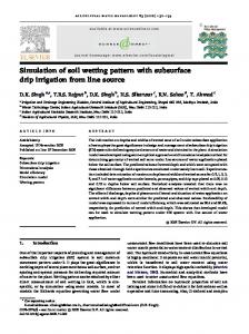
List of Figures Figure 1.1. An input response curve for water or fertiliser. The penalty of under supply of inputs is severe when the input response curve is steep. The uncertainty of position B and the cheap cost of inputs drive the farmer towards point C (From Stirzaker 1999). ....................................................................................... 1 Figure 1.2. a) The electronic prototype contains a float switch behind the filter. If the cell containing the float fills completely, water overflows into a storage reservoir and this sample can be extracted for nutrient or salt monitoring. Water around the float switch is withdrawn back through the filter by capillary action as the soil dries, thus resetting the detector. b) The mechanical prototype has a narrow reservoir below the filter which houses a styrofoam float. As the reservoir is filled the float moves up the float housing and protrudes above the soil surface. The reservoir is emptied by syringe through an extraction tube................ 4 Figure 2.1. The relationship between the amount of drip irrigation (left axis) and number of detectors that responded to each irrigation (right axis). The open bars at the right represent rainfall, not irrigation........... 7 Figure 2.2. The response of detectors to rainfall during the early stages of the garlic crop. The solid line shows the cumulative rainfall over a three-day period. The horizontal bands denote the period when the first and last detectors at depths of 200 and 300 mm responded. The horizontal band on 14 June shows the period in which all detectors responded after rainfall resumed................................................................................. 9 Figure 2.3. The change in nitrate-N measured from samples stored in the detectors at 300 mm from the drip irrigated pumpkin crop. ................................................................................................................................ 10 Figure 2.4. The change in nitrate-N measured from samples stored in the detectors at 200 and 300 mm from the sprinkler irrigated garlic crop (left axis). The line without symbols shows the cumulative rain plus irrigation (right axis). ................................................................................................................................... 10 Figure 2.5. The response of detectors (right axis) to irrigation amount (left axis) in the pumpkin crop from sowing to harvest. The total number of detectors was ten. .......................................................................... 11 Figure 3.1. The depth of the tensiometers, suction cups, TDR and WFD placement at each site. The soil texture changed from sandy loam to clay at around 300 mm depth............................................................. 13 Figure 3.2. The daily average volumetric water content over the 0-400 mm depth at five sites .......................... 15 Figure 3.3. The hourly change in volumetric water content averaged over the five sites for three irrigation cycles............................................................................................................................................................ 16 Figure 3.4. The maximum TDR readings after irrigation compared to the number of detectors at 300 and 400 mm that responded. ...................................................................................................................................... 16 Figure 3.5. The change in nitrate-N concentration from a) suction cup sampled b) WFD samples analysed in the laboratory c) suction cup samples measured with test strips d) WFD samples measured with test strips. ............................................................................................................................................................ 18

vi

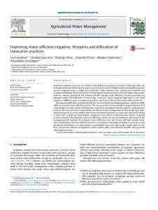
Figure 3.6. ............................................................................................................................................................. 19 a) The amount and distribution of irrigation or rainfall during the dam, bore and no irrigation phases ...... 19 b) The EC of samples from suction cups ..................................................................................................... 19 c) The EC of samples from WFDs ............................................................................................................... 19 d) The EC as measured by TDR................................................................................................................... 19 Figure 4.1. Cumulative irrigation and rainfall (left axis), and soil deficit to 100 cm (right axis) for the pivot irrigated corn crop. The arrows denote the time that detectors were activated. The number alongside each arrow e.g. 4/2 denotes that 4 detectors were activated at a depth of 25 cm and 2 detectors were activated at a depth of 50 cm. ...................................................................................................................................... 24 Figure 4.2. The soil water profile at early in the season (squares) mid-season (triangles) and end of season (diamonds).................................................................................................................................................... 24 Figure 4.3. The concentration of nitrate (mg/l) removed from detectors at 25 cm (blue line) and 50 cm (red line) and the application of nitrogen fertilizer (kg/ha N). ............................................................................ 25 Figure 4.4. Cumulative irrigation and rainfall (right hand axis) and the soil water deficits to 40 and 100 cm (left hand axis) ..................................................................................................................................................... 27 Figure 4.5. The duration of irrigation and time taken for the four WFD to respond after the irrigation was switched on during periods A, C and D of Fig. 4.4...................................................................................... 28 Figure 4.6. The bean crop at Tatyoon showing the logger box which was connected to six wetting front detectors in the same row ............................................................................................................................. 29 Figure 4.7. The stored water in the top 100 cm from replicate diviner tubes ....................................................... 30 Figure 4.8. Evaporation plus drainage calculated from the irrigation record and changes in soil water measured by the Diviner............................................................................................................................................... 31 Fig. 4.9. The actual amount of water applied (blue line), and the amount that would have been applied had the 40 cm detector automatically controlled irrigation....................................................................................... 31 Figure 5.1. The trials were carried out in conjunction with Dr Ping Lu, CSIRO Plant Industry (right). The farm owner (centre is holding a mechanical wetting front detector ..................................................................... 33 Figure 5.2. Holes were dug with a 20 cm and 5 cm diameter auger for installation of detectors ......................... 34 Figure 5.3. The application rate (mm/h) between two adjacent mini-sprinklers at the top and bottom of the block............................................................................................................................................................. 35 Figure 5.4. The water content (m3m-3) measured by TDR over the 300-600 mm depth at two sites during the 02/03 season (continuous lines). The four broken horizontal lines show the times that each of the four wetting front detectors contained water. A point denotes that the detector tripped and reset within a few hours............................................................................................................................................................. 36 Figure 5.6. The water content over the 0-300 and 300-600 mm zones measured by TDR and the time each of four wetting front detectors detected the arrival (start of line) and removal of water (end of line) in the base of the funnel. ........................................................................................................................................ 37 Figure 6.1. Average daily irrigation rates for the 17 growers. There is considerable scatter, partly because the data does not all cover the same time period................................................................................................ 40 Figure 6.2. Simulations showed that it would take around 8 hours for a wetting front from a 2.7 l/h dripper to reach 50 cm, even starting from a moist soil for a sand (left) or loam soil (right). According to the model the irrigation system would need to be run for over 24 hours to activate a 100 cm deep detector. ............. 50

vii

Executive Summary Surveys have shown that there is a poor relationship between water applied and yields obtained for the same crops in the same district, demonstrating there is much room for improving the management of irrigation. There are already tools and services available for monitoring soil water and the solutes it contains, but the majority of irrigators do not make use of them. We contend that poor adoption is related to the cost and complexity of soil water monitoring, rather than any intrinsic fault in the tools themselves i.e. the barriers to best practice are as much socio-economic and cultural as they are technical. Low cost and simplicity are essential to breach the impasse of poor adoption. However simplicity cannot be at the expense of accuracy, so we need to find the balance between simplicity, accuracy and cost for improving water and nutrient management from a low base. This project introduces the FullStop wetting front detector to farmers and evaluates its performance on a range of farms under surface drip, buried drip, fixed sprinkler, centre pivot and mini-sprinkler irrigation on a variety of annual and perennial crops. The wetting front detector is a funnel-shaped instrument that is buried in the soil. The funnel concentrates the downward movement of water so that saturation occurs at the base of the funnel. The free (liquid) water produced from the unsaturated soil activates an electronic or mechanical float, alerting the farmer that water has penetrated to the desired depth. The detectors retain a sample of soil water that is used for nutrient and salt monitoring. Irrigation scheduling is often portrayed by scientists as an exercise in accuracy - the idea that there is a defined refill point and upper drained limit and a precise amount of water can be added to satisfy the crop without wastage. Things look different on the farm; irrigators are aware of non-uniformity in their irrigation systems and variability in soils and plant growth. Moreover they often cannot irrigate exactly on cue because water is being used elsewhere on the farm or some other cultural operation requires the irrigation to be withheld. Since many other tasks compete for their attention, the key issue from the farmer’s point of view is the value of information relative to the time and expense involved in getting the information. The case studies showed that the wetting front detector helped irrigators to evaluate their own practice and challenged their perceptions of what was happening in the root zone. In several cases the detectors quickly honed in on the most important issues to be addressed by the farmer, which is the art of troubleshooting. Detectors do not provide quantitative data, but help irrigators to move in the right direction; after all the soil is a buffer and it is not important to be right every time – just important not to be consistently wrong. Perhaps the most tantalising aspect of this research project was the ability of the detector to provide information on the electrical conductivity and soil nitrate in the root zone from the water sampled from the wetting front. Wherever we monitored EC of nitrate in the case studies above, it proved to be highly instructive. The use of simple colour test strips for nitrate and portable EC meter means that a water sample can be tested in-field in less than two minutes for a cost of under $1. The management of water, salt and nitrate are inextricably linked and it is not possible to be on the “clean and green” road without monitoring all three. In most of the case studies water was independently monitored by tensiometer, gypsum block, capacitance probe or time domain reflectometry to evaluate the accuracy of the detector. Weak redistributing fronts can pass the detector without activating it – and this was observed - but on the whole the evidence was that the wetting front detector was sufficiently accurate to improve irrigation management.

viii

The wetting front detector is best seen as a learning tool. Wherever it was deployed it aroused curiosity and opened up a dialogue between farmer and scientist. Because the dynamics of water, salt and nitrate in the soil are complex, this dialogue needs to be facilitated if we want to see sustained change. Social researchers know that change is a complex process consisting of many steps, including pressure for change, the vision for change, capacity to change, actionable first steps, roles models and the like. The wetting front detector can start the process. It proved to be a simple way of showing irrigators how deep wetting fronts penetrated into the soil and the solutes moving with them. We conclude that a simple tool can stimulate irrigators to re-evaluate their practices and help them to take another step along the difficult road of managing water and the solutes it contains.

ix

x

Chapter 1: Introduction to the farmer’s road toward clean and green horticulture The slogan that Australian agricultural produce is clean and green is powerful marketing tool. The claim of “clean” is largely justified; stringent tests are in place to ensure that food is free of contaminants and are rarely breached. The claim of “green” is much harder to substantiate. “Green” suggests the productions methods are environmentally benign, a position hard to justify in the light of the recent Land and Water Audits and State of the Environment reports. To say that farming practices are not green is not in itself a criticism of the farming community. Australia is, for the most part, a difficult environment to farm. In the case of irrigation, the availability of water and best soils for irrigation often do not coincide. Moreover, irrigation areas are often underlain by large scale aquifers with very low discharge capacities, leaving little room for the leaching of salts required for sustainable practice. The biophysical environment is harsh, but the problem is compounded by the socio-economic factors surrounding irrigation. Even though water is the primary constraint to horticultural production, it is the cheapest to deal with, usually less than 5% of the total variable costs. The low cost of water relative to the value of horticultural crops gives rise to a steep input response curve. A “‘green” farmer would want to operate around point B in Fig. 1.1, with a bit extra input to cover the uncertainty of where the flat part of the curve begins. Herein lies the farmer’s dilemma. Available water and nutrients, particularly nitrogen, fluctuate widely over short periods. Though the technology is available to monitor these changes, few farmers have the time, money or skill to carry out such monitoring in an accurate way. Because of the uncertainty of location position B, and the fear of sliding down the response curve to point A, the common strategy is to operate closer to point C. An extra 100 mm of water plus 50 kg of nitrogen is cheap insurance for a crop with a gross value of many thousands of dollars (Stirzaker 1999). However the water and nutrients not used by the crop can become pollutants in the receiving ecosystems, throwing into question the green label.

Figure 1.1. An input response curve for water or fertiliser. The penalty of under supply of inputs is severe when the input response curve is steep. The uncertainty of position B and the cheap cost of inputs drive the farmer towards point C (From Stirzaker 1999). Scientists tend to view Fig. 1.1 within an accuracy framework i.e. a precise determination of point B. From the farmer’s perspective, change incurs risk of under-irrigation, and so there needs to be a process during which information reduces the risk to the point that the farmer is willing to alter

1

practices (Pannell and Glenn 2000). This report views the dilemma shown in Fig. 1.1 from the farmer’s side – the nexus between information and risk – hence the Title “The Farmer’s Road to Clean and Green Horticulture”. The aim was to assist farmers on the journey by providing them with a simple new device called a wetting front detector which provides basic information on water, nitrate and salt management.

Objectives The project had two objectives • Provide the land manager with simple devices to evaluate their own performance in managing water, salt and nutrients in irrigated horticulture. • Assist land managers to monitor the benefits of adopting new practices worthy of the clean and green label

Methodology The methodology was to 1. Install detectors in farmers’ fields 2. Transfer the information on wetting front depths and solute concentration to the farmer in a way they can understand 3. Use the information to initiate the process towards change of practice and evaluate the impact of changed practices.

The Wetting Front Detector The detector works on the principle of flow line convergence. Irrigation water or rain moving downwards through the soil is concentrated when the films of water moving around soil particles enter the wide end of the funnel. The soil in the funnel becomes wetter as the funnel narrows and the funnel shape has been designed so that the soil at its base reaches saturation when the wetting front outside is at a similar depth. Once saturation has occurred free water flows through a filter into a small reservoir and activates a float (Stirzaker et al 2000, Stirzaker 2003). The wetting front detector can be used to schedule irrigation because the time it takes for water to reach a certain depth depends on the initial water content of the particular soil (Philip 1969). If the soil is dry before irrigation, the wetting front moves slowly because the water must fill the soil pores on its way down. Therefore a lot of water is needed before the detector will respond. If the soil is quite wet before irrigation, then the wetting front will move quickly through the soil. This is because the soil pores are already mostly filled with water so there is little space for additional water to be stored. Thus a short irrigation will cause the detector to respond. The float in the detector is activated when free water is produced at the base of the funnel. Water is withdrawn from the funnel by capillary action after the wetting front dissipates. Depending on the version used, capillary action can be used to “reset” the detector automatically, or water can be removed via a syringe. The water sample can be used for routine salt and fertilizer monitoring.

The Early Experiments The original version of the wetting front detector contained two electrodes behind a filter in the neck of a funnel. The water passing through the filter completed the circuit between the two electrodes, thus providing the signal that the wetting front had reached the detector. This system proved to be very robust, but a cheaper solution was to replace the conductivity cell with an electronic float switch. The float switch could be connected in series with any commercially available irrigation controller and a solenoid valve. The solenoid valve would open according to the start time set on the controller and the

2

detector could override the run-time. For example, if the wetting front reached the desired depth before the end of the designated run time, the float switch would rise, thus breaking the circuit between the controller and the solenoid. The first field experiments were carried out on a research station. Four detectors were placed at a depth of 15 cm under sprinkler irrigated turf. Irrigation was turned on automatically on a four to seven day interval, depending on the time of the year. When three of the four detectors recorded the arrival of the wetting front the irrigation was automatically shut down. The method proved to be surprisingly accurate. Each irrigation event filled the profile to almost exactly the same point (as measured by Time Domain Reflectometry) and there was a very slight drying down of the 30 – 50 cm zone, indicating that the turf was not over-irrigated (Hutchinson and Stirzaker 2000). Further experiments on other soil types also gave good results (Stirzaker 2003) and this provided the confidence that the detectors were reliable and the method of irrigation scheduling by position of the wetting front was a sound one (see also Zur et al 1994).

The Farmer’s Road Despite the success on the experimental farm, the method of irrigation scheduling would not suit the majority of farmers. One of the most important factors determining farmer adoption of a new technology is their ability to try it out and “see if it works for them” (Pannell 1999). Few farmers have irrigation controllers and electronic valves that can be automatically shut down by a detector. For those who do, it is a considerable risk to hand over control to a buried device with batteries and wires. Whereas conventional soil monitoring equipment provides information to the manager but a WFD in control mode takes over the management. Something as simple as a broken wire could spell disaster. The best way to make something easy to trial is to make it simple. That meant removing the conductivity cell or electronic float switch from the detector (Fig. 1.2a) and turning it into a completely mechanical device. In the modified version, free water is collected in a narrow reservoir and floats a stick of Styrofoam thus providing a visual signal to the farmer that the wetting front had reached the detector. Farmers could observe the float and evaluate their irrigation practice (Fig. 1.2b). The automatic control method is not ‘farmer friendly’ for a second more complex reason; a considerable amount of knowledge is required to correctly choose the placement depth and irrigation interval and if these are wrong the automatic control will not be accurate. To get the depth and interval right requires an understanding of the concept of redistribution of water after irrigation (see Appendix 1). When water infiltrates through the soil and sets off a detector, the soil water content is well above field capacity, and redistribution of water will occur to deeper layers. The amount of water moving past a detector depends on how much water there is to redistribute, which itself is a function of irrigation method, soil type, irrigation rate and detector depth.

3

a)

b) Float Float housing

Funnel

Overflow

Filter

Float switch

Reservoir Filter Sample extraction tube

Storage reservoir

Extraction tube

Figure 1.2. a) The electronic prototype contains a float switch behind the filter. If the cell containing the float fills completely, water overflows into a storage reservoir and this sample can be extracted for nutrient or salt monitoring. Water around the float switch is withdrawn back through the filter by capillary action as the soil dries, thus resetting the detector. b) The mechanical prototype has a narrow reservoir below the filter which houses a styrofoam float. As the reservoir is filled the float moves up the float housing and protrudes above the soil surface. The reservoir is emptied by syringe through an extraction tube. Redistribution of water makes it difficult to know how deep water penetrates after a Wetting Front Detector has shut down the irrigation. If the detector is deep and the irrigation interval short, water might still be draining from the lower part of the profile when the next irrigation starts. This will lead to over-irrigation. Conversely, if the detectors are shallow and the irrigation interval is long, the crop might be under-irrigated. To overcome these problems we set up detectors in pairs, a shallow detector about one third of the way down the managed root zone and a deeper detector about two thirds down the managed root zone (the managed root zone is the maximum depth of soil that the irrigator wants to replenish with water). Early on in the season the shallow detector should respond occasionally to irrigation. This is a time when nitrate leaching is common and over-irrigation must be avoided. As the crop grows the shallow detector should respond to most irrigation events, to ensure that the wetting front is penetrating to the middle and lower portion of the active root zone. The deeper detector should respond from time to time: if it never responds we may be slowly drying the profile out. If the deep detector responds to every irrigation event we are over-irrigating. This report is largely about testing the above ideas with the simple version of the detector shown in Fig. 1.2b. Irrigators were given mechanical wetting g front detectors and we then followed them through the experience of using them. In a number of cases electronic detectors which were logged were also installed. By monitoring the actual irrigation times of the farmer via a pressure transducer inserted into the irrigation lines, the electronic detectors gave a more detailed picture of when detectors tripped and reset and reduced the reliance on farmer records. In some of the case studies the farmers already relied on their own scheduling equipment, so the response of the detector was compared to that. Where there was no independent method of monitoring soil water we installed our own equipment. The chapters that follow focus on a quantitative assessment of the performance of the wetting front detector in real farm situations. However there

4

were many farmers loosely connected to the project that contributed valuable experience and these have been included where possible. Chapter 2 provides a summary of the learning experience after using detectors for two seasons. The focus is on how the detectors changed farmer perceptions about irrigation and highlighted the critical aspects to get right. Chapter 3 is a comparison of methods for monitoring water, nitrate and salt on farm. Whereas the main aim of the wetting front detector project is to produce a tool that is simple to understand and cheap to purchase, it must also pass the accuracy test. The focus is on how the amount, complexity and accuracy of information effects the day to day decisions made on the farm. Chapter 4 widens the range of irrigation methods tested by evaluating centre pivot and buried drip irrigation as a contrast to the surface drip and solid set sprinkler systems in the previous chapters. Chapter 5 evaluates the performance of detectors under mini-sprinklers on a perennial crop, as opposed to the annual vegetable crop above. Mini-sprinklers can be a special case because they have low application rates, which might result in wetting fronts that are difficult to detect, and high variability in the wetting patterns. Chapter 6 evaluates a case where an irrigator association wanted to use the wetting front detector as part of their accreditation process. The experiences of a number of different growers with different irrigation strategies are compared. Chapter 7 provides an overview of the lessons learnt and recommendations.

5

Chapter 2: Four lessons from a wetting front detector Introduction Against the background of poor adoption of irrigation scheduling tools by farmers, the FullStop wetting front detector was developed in answer to the question “what is the simplest information that would help an irrigator make a better decision?” (Stirzaker et al. 2000). In a range of experimental trials, the wetting front detector performed well in comparison to other methods of scheduling (Hutchinson and Stirzaker 2000, Stirzaker 2002). This paper evaluates how useful the detectors were in the hands of irrigators. The evaluation took place on a small market garden near the town of Gundaroo in the Southern Tablelands of NSW. A range of high quality organic vegetables is direct marketed to subscription clients and restaurants. The owners had not used irrigation scheduling tools before, but were highly motivated to save water both because of limited supply and their commitment to environmental stewardship. They were keen to use the wetting front detector because of its simplicity and low cost. In previous work the wetting front detectors had been used in “control” mode. Electronic detectors were connected to solenoid valves and automatically shut off irrigation when the water reached the required depth. The “control” method worked well, but its success depended on choosing the right combination of detector depth and irrigation frequency. In this study wetting front detectors were used as a learning tool; that is the farmers started with their own experience, and then modified their practice according to feedback from the detectors.

Materials and Methods The soil was a red chromosol with a sandy loam topsoil 300 mm deep overlying a light clay. The pumpkin crop Cucurbita pepo var delicata was planted on 30 December 2000 on raised beds spaced 1 m centre to centre. Each bed had a row of drip tape with 2 l/h emitters spaced 0.5 m apart, with seeds planted adjacent to each emitter. Compost was added before planting at a rate of approximately 60 m3/ha. This was incorporated in the top 200 mm of soil. The pumpkin crop was harvested on 20 March 2001, and the crop residues removed. The beds were reformed, compost added at the same rate as above. The drip irrigation was removed and sprinklers set up with an application rate of between 10-15 mm/h. Garlic Allium sativum was planted in 4 rows per bed with 100 mm between the bulbs on 25 April. Ten electronic wetting front detectors and five mechanical detectors were installed in the pumpkin crop. All detectors were placed with the rim of the funnel 200 mm below the soil surface directly below an emitter. Earlier work showed that the detectors record the wetting front when it is approximately 100 mm below the rim of the funnel, hence the depth of measurement for this crop was 300 mm. The electronic detectors were connected to a Campbell Scientific CR10X logger that recorded the time the float was up (water in the detector) and time the detector reset (water withdrawn from the detector by capillary action). The time and duration of irrigation was logged by a pressure transducer and rainfall logged using an automatic rain gauge. One emitter was connected to a short length of 4 mm tubing and placed directly into the rain gauge to monitor variations in irrigation rate. Ten electronic and ten mechanical detectors were set up in pairs for the sprinkler irrigated garlic crop. The upper detector of each pair monitored wetting fronts at a depth of approximately 200 mm and the

6

deeper detector at a depth of 300 mm. Electronic detectors, rainfall and irrigation were logged as above. The farmers remained in complete control of the irrigation timing and duration. The mechanical detectors send up a float to give a visible indication that water has reached them. This information was immediately available to the farmers and influenced subsequent irrigations. The logged record was viewed several times during each crop, which further influenced their irrigation decisions. Water samples were removed from the detectors at weekly (summer) or fortnightly (winter) intervals. Nitrate test strips (Quantofix, Macherey-Nagel, Duren) were used to give an immediate approximate measure of the concentration of nitrate moving past the detectors.

Lesson #1: Drip - shorten the interval between irrigation events The detector installation depth of 300 mm in the drip-irrigated pumpkin crop was chosen because it marked the transition between the topsoil and subsoil. Since fewer roots were observed in the subsoil, it was reasoned that there was little point in pushing wetting fronts below 300 mm if the water might subsequently be difficult for young plants to extract. The very first irrigation showed how difficult this goal could be. Just 14 minutes of irrigation, or 612 cm3 per emitter, was enough to activate five out of ten electronic detectors at 300 mm. On an area basis this equated to an irrigation depth of 1.2 mm (Fig. 2.1). The next irrigation on January 5 was 0.7 mm, and only one detector responded. Two days later an irrigation of 1.1 mm set off seven of the ten electronic detectors. Over the first three weeks it became clear that 1-1.5 mm (12-18 minutes) would set off 5 to 7 detectors; less than 1 mm would set of just one or two of the ten. Clearly very small changes in irrigation elicited a large response from the detectors. 16

10 Irrigation Dectectors

8

12 10

6

8 4

6 4

# Detectors

Irrigation/rain (mm)

14

2

2 0

0 2-Jan

9-Jan

16-Jan

23-Jan

Figure 2.1. The relationship between the amount of drip irrigation (left axis) and number of detectors that responded to each irrigation (right axis). The open bars at the right represent rainfall, not irrigation. Rain on January 25 demonstrated the difference between complete and partial wetting of the soil surface (open bars in Fig. 2.1). Rainfall of 11.7 mm was not sufficient to set off any detectors, and a further 14.8 mm the following day still had no impact. It took 25.1 mm of rain a week later set off 3 detectors, before a large rainfall event of 31.9 mm set off nine of the ten detectors. 7

There are two reasons for the small amounts of drip irrigation required during the early stages. First, the diameters of the wetting patterns averaged 20 cm, representing 6 % of the soil surface. Second, the only loss of water was soil evaporation from the small wetted area and some transpiration from the seedling. Once a detector had tripped, the soil between 100 and 300 mm remained close to the upper drained limit. Wetting fronts move quickly through wet soil, hence the short irrigation required.

Lesson #2: Sprinkler irrigation – lengthen the duration of each event Rain during the drip irrigated pumpkin crop had already alerted the farmer to the fact that more than 15 mm was required to get the wetting front down to 300 mm, unless the soil was very wet. The actual amount of water required is a function of initial water content of the soil. This is the principle behind the operation of the wetting front detector. For a given soil/irrigation rate combination, the speed of propagation of the front is proportional to the initial water content (Philip 1969). Dry soil would therefore require a long irrigation and wet soil a short irrigation. Detectors were placed at depths of 200 and 300 mm for the sprinkler irrigated garlic crop. It is preferable that wetting fronts do not penetrate as deep under sprinkler as they do under drip irrigation. This is primarily because the entire soil area is wetted by sprinklers. A second reason relates the way soil water redistributes after irrigation has ceased. Under drip irrigation, water is pulled sideways by capillarity as well as downwards. Under sprinkler irrigation, all redistribution is downward. The garlic crop was planted in late autumn, and no irrigation was required until late spring. Fig. 2.2 gives an example of how the detectors responded to rainfall during the early stages. Over an 18 hour period there was 23.9 mm of rain falling at a fairly constant rate of 1.3 mm/h. The soil was moist prior to this, as rain had fallen four days earlier. All five of the electronic detectors at a depth of 200 mm responded after 9.1 to 11.2 mm of rain. The five electronic detectors at 300 mm responded after 12.8 - 23.3 mm. After a break of 18 hours the rain started again with a further 4 mm. In this case all ten detector at 200 and 300 mm responded after just 2.1 – 3.5 mm. This illustrates the point concerning initial water content and amount of water needed to trip the detectors. It took 23.3 mm to trip all detectors when the soil was moist, and just 3.5 mm when the soil was very wet. Five sprinkler irrigations were applied in the spring/summer. Though the weather was now warm and the crop at maximum leaf area, the detector record shows that, in general, too much water was applied. For each irrigation except 22 November, all five detectors at 200 mm were activated. On 20 Oct, 6 Nov and 28 Nov three or more detectors at 300 mm were activated. This demonstrates that water was moving past 300 mm and into the clayey subsoil. From this small data set, it appears 20-30 mm per irrigation would be appropriate. The interval between irrigations could be lengthened if more detectors responded and shortened if fewer responded the previous time.

8

35

Rainfall (mm)

30 all detectors responded

25 20

300 mm responded

15 10

200 mm responded

5 0 12-Jun

13-Jun

14-Jun

15-Jun

Figure 2.2. The response of detectors to rainfall during the early stages of the garlic crop. The solid line shows the cumulative rainfall over a three-day period. The horizontal bands denote the period when the first and last detectors at depths of 200 and 300 mm responded. The horizontal band on 14 June shows the period in which all detectors responded after rainfall resumed. Table 2.1. The dates and amount of irrigation water applied to the garlic crop and the number of mechanical detectors that responded at 200 and 300 mm. Date

Irrigation (mm)

# FullStops 200 mm 5 5 4

# FullStops 300 mm 4 5 1

20 Oct 35.5 6 Nov 49.5* 22 23.4 Nov 28 46.9 5 3 Nov 5 Dec 39.8 5 1 *16 mm irrigation followed by 33.5 mm rain

Lesson #3: Nitrate leaching when the crop is young Each time a wetting front is detected, a sample of water is retained in the detector. This sample was used for rapid assessment of the nitrate status of the soil using nitrate test strips. At the start of the season the nitrate-N levels were high for both crops, even though no artificial fertilisers were used (Fig. 2.3). In the case of the drip irrigated pumpkin crop nitrate-N dropped from 60 to 23 mg/l during the early crop stage when total irrigation was only 10 mm. Thereafter nitrate N remained fairly constant before falling sharply again during the period of exponential growth. It is important to note that the nutrient concentrations would be much higher in the 80% of the soil volume outside that wetted by the drip emitters. Thus the timing of rainfall and hence water and nutrient uptake would have an enormous impact on crop nutrition.

9

Nitrate-N (mg/l)

80 60 40 20 0 30-Dec

19-Jan

8-Feb

28-Feb

Figure 2.3. The change in nitrate-N measured from samples stored in the detectors at 300 mm from the drip irrigated pumpkin crop. Fewer water samples were available from the garlic crop. Since it was not irrigated during the early stages, samples could only be collected after rain. Nevertheless nitrate-N levels fell sharply after the rains in early June. The nitrate-N levels at 200 mm were quite low by early August, but still moderate at 300 mm, indicating that the topsoil had not been fully flushed (Fig 2.4). The nitrate-N level at 300 mm had fallen to low levels by mid October, the period when the crop was growing rapidly. 600

120 N-200 Rain+ Irrig

400

60 200 30

0 9-Apr

Rain + Irrig (mm)

Nitrate-N (mg/l)

N-300

90

0 9-Jun

9-Aug

9-Oct

9-Dec

Figure 2.4. The change in nitrate-N measured from samples stored in the detectors at 200 and 300 mm from the sprinkler irrigated garlic crop (left axis). The line without symbols shows the cumulative rain plus irrigation (right axis).

Lesson #4: Misjudging the onset of exponential growth The pumpkin crop was irrigated every second day during the first month. With one exception, the first nine irrigations activated 5 or more detectors. The subsequent nine irrigations activated 2 detectors or less. Even after the heavy rain on 4 and 5 February, when the soil profile was fully wetted, too little irrigation was given. It was not until 14 February, when the irrigation amount was increased to over 6 mm and the interval shortened to daily, that five or more detectors were consistently activated (Fig 2.5).

10

10

12 Irrigation Detectors

8

8

6

6 4

4

2

2 0 30-Dec

# Detectors

Irrigation (mm)

10

0 13-Jan

27-Jan

10-Feb

24-Feb

10-Mar

Figure 2.5. The response of detectors (right axis) to irrigation amount (left axis) in the pumpkin crop from sowing to harvest. The total number of detectors was ten. The rapid escalation in water use, from around 0.5 mm/day in mid January to 5 mm/day in mid February reflects the period of exponential vegetative growth. The crop was also growing into increasing temperatures. Flowering and fruit set occur during the latter part of this period, the time when the yield of many vegetable crops is most susceptible to water deficits (e.g. Rudich et al. 1977). Thus, if stress is going to occur at all, it is most likely to occur when the yield is most vulnerable, as deficits accumulate over the exponential growth period.

Conclusion Irrigation scheduling is often portrayed by scientists as an exercise in accuracy - the idea that there is a defined refill point and upper drained limit and a precise amount of water can be added to satisfy the crop without wastage. Things look different on the farm. There are clear differences in the size of plants hence transpiration, especially during the early stages of growth. The drip emitters in this study were rated at 2 l/h but varied between 2.3 and 2.7 l/h. The sprinklers were less uniform. Farmers are well aware of this variability. Moreover they often cannot irrigate exactly on cue, either because water is being used elsewhere on the farm, or some other cultural operation requires the irrigation to be withheld. Of greater importance, the farmer must optimise many tasks simultaneously, from soil preparation to marketing. The key question from the farmer’s point of view is what is the value of information in reducing uncertainty, and what does it cost to get that information (Pannel and Glenn 2000). In this study the wetting front detectors quickly honed in on the most important issues to be addressed by the farmer, as outlined in the four lessons above. They did not resolve the question of accuracy, but helped the farmer to move in the right direction. After all the soil is a buffer and each irrigation event need not be accurate. It is not important to be right every time – just important not to be consistently wrong. In the words of the farmer involved in this trial, “the detectors provided a point of dialogue between the experience of the farmer and the language of the scientist”. Essentially the detectors are a learning tool. They help the irrigator to evaluate their own practice and to modify this practice as their knowledge and confidence grows.

11

Chapter 3: Monitoring Water, Nitrate and Salt on-farm: a comparison of methods Introduction A scientific comparison of methods is usually a test of accuracy; one method has been accepted as a standard, and a newer approach must equal or better the incumbent. A recent review by Charlesworth (2000) showed that there are over 20 soil water monitoring tools available, so it is reasonable to ask which are the most accurate. Yet survey data shows that at least 85% of irrigation farmers do not make use of any scientific tool (Australian Academy of Technological Sciences and Engineering 1999) and there is little evidence that accuracy or lack of it is the problem. According to Blacket (1996), scientists frequently fail to get farmers to adopt their products because they frame the problem around their own world view, not the world view of their clients. In the face of sustained poor adoption, the question for scientists is what information would be most useful to irrigators. To answer this we must determine how an irrigator translates information into management decisions. This study compares Time Domain Reflectometry (TDR), Wetting Front Detectors (WFD) and tensiometers for monitoring soil water status in a vegetable crop. Suction cups were also installed for the collection of soil solution, and the samples collected from suction cups and WFDs were analysed for nitrate concentration and electrical conductivity (EC). Since the TDR can also measure bulk soil EC, the trial had three methods for monitoring EC as well as three for monitoring soil water status. Nitrate in water samples from suction cups and WFDs was measured accurately in the laboratory or estimated in the field from colour test strips. The trial was run together with the farmer to answer the following questions 1. Can the information from the monitoring tools be directly related to yield and hence profit? 2. Does the information increase our ability to make better management decisions? 3. Does an increase in the volume or accuracy of information alter the management decision?

Materials and Methods Silverbeet (Beta vulgaris) was grown in double rows on raised beds spaced 1 m centre to centre under sprinkler irrigation on a farm near Gundaroo, NSW. The soil was a red chromosol with a sandy loam topsoil 300 mm deep overlying clay. Five locations were chosen in the field that varied in distance to the nearest sprinkler, and TDR, WFDs, tensiometers and suction cups were installed at each site (Fig. 3.1). TDR: Two TDR probes (Zegelin et al 1989) were installed vertically into the soil at each site to provide continuous measurement of volumetric soil water content. The probes were installed from the surface to 200 mm and 400 mm to give the average water content over the 0-200 mm and 0400mm depths of soil. Measurements of water content and EC were made hourly. WFD: The wetting front detectors (Stirzaker 2003) were the mechanical version having a float visible at the surface to provide the signal that a wetting front had reached the prescribed depth. Detectors were placed to measure fronts at 200 mm, 300 mm and 400 mm depths at each site. Experience has shown that the detector records a wetting front when it is about 100 mm below the rim of the funnel,

12

so the rim was located 100 mm above the prescribed depths (see Fig. 3.1). The detectors needed about 15 ml of water to activate the float and this was recorded after each irrigation event. Tensiometer: The tensiometers had a porous ceramic cup with a length of 60 mm and diameter of 20 mm. They were installed with the midpoint of the ceramic cup at 200 mm and 400 mm depths at each site. The tensiometers had a rubber septum which was pierced with a hypodermic needle and the tension recorded on a pressure transducer according to the method of Cresswell (1993). Readings were taken before irrigation and within 24 hours after irrigation. Suction cups: The suction cups had a porous ceramic cup with a length of 60 mm and diameter of 40 mm. They were installed with the midpoint of the ceramic cup at 200 mm 400 mm depths. A suction > 70 kPa was applied to each cup within 24 hours after each irrigation event and the suction cup was then sealed for four hours before sampling the fluid.

Figure 3.1. The depth of the tensiometers, suction cups, TDR and WFD placement at each site. The soil texture changed from sandy loam to clay at around 300 mm depth. All the equipment was installed on 7 November 2003, except for the 200 and 300 mm depth wetting front detectors which had been installed a year earlier. Installation was carried out with an auger of slightly greater diameter than each instrument, and the soil repacked, ensuring good contact in the case of the suction cups and tensiometers. Silverbeet seedlings were transplanted on 26 November and two weeks later chopped lucerne hay applied as mulch around the seedlings. The farm followed the principles of organic farming. Previous crops had received compost, and the silverbeet crop received 7.5 t ha-1 lucerne mulch containing 2.76% N or 207 kg N ha-1. Irrigation was carried out once per week and water samples taken within 12 to 24 hours after irrigation ceased. The general irrigation strategy was to turn off the water when the detectors at 300 or 400 mm depths first started to respond. Dam water was used for the first half of the season and bore water, with an electrical conductivity of 1.5 dSm-1, used during the second half. The electrical conductivity of the water samples from the WFDs and suction cups was measured with a CDM83 conductivity meter (Radiometer, Copenhagen) and the nitrate content measured using a segmented flow analyser (Alpkem 1992) or estimated from nitrate test strips (Quantofix, MachereyNagel). Soil samples were also taken from the 0-200 and 200-400 mm depths from each site prior to planting for nitrate analysis.

13

Ten plants growing over each of the monitored sites shown in Fig. 3.1 were non-destructively sampled by removing all fully expanded leaves, which were then dried at 70 oC and weighed. Sampling was carried out on five occasions, the first on 8 January and the last on 23 April 03.

Results Water The period up to 8 January was considered the establishment phase, and all data relates to the measurements since that date. The total rainfall between 8 Jan and 23 April was 406 mm and total rainfall 105 mm, giving 4.9 mm d-1. The aim was to irrigate once per week and since there was only one rainfall event greater than 12 mm, this was usually possible. The data in Table 2.1 summarises the tensiometer, WFD and TDR data over 12 irrigation events and one rainfall event. The cumulative yield of silverbeet varied from 3.25 t DM ha-1 (Site 5) to 5.02 t DM ha-1 (Site 3), and yields are expressed as a percentage of the Site 3 value in Table 3.1. The WFD response in Table 3.1 was calculated as percentage of maximum possible activation of detectors. Each site was given a score of 1 if the 200 mm detector was activated and score of 2 if the 200, 300 and 400 mm depths were activated. Sometimes wetting occurred more effectively via the furrows between beds than through the surface of the bed and deeper detectors were activated but not shallow ones. In this case 0.5 points were given for each of the 300 and 400 detectors activated, since each represented one quarter of the managed root zone (200 -300 mm and 300 – 400 mm). The score for each site is the sum of detector responses out of a possible 26 for the 13 events studied, expressed as a percentage. The tensiometer data is the suction at 400 mm depth prior to irrigation, and thus is an indicator of the maximum stress. The TDR data is the average of all the hourly water content measurement over the 105 day period for each site, expressed as mm of water in the top 400 mm of soil. Table 3.1. The relative yield of silverbeet averaged over four harvest dates, the average soil suction at 400 mm depth prior to irrigation, the WFD response rate after irrigation and the average water stored in the top 400 mm measured by TDR Site number

S3 S1 S4 S2 S5

Yield

% 100 91 88 79 65

Tensiometer max suction at 400mm kPa 14 10 23 34 42

WFD Response after irrigation % 92 67 81 63 56

TDR Water stored in top 400 mm Mm 92 75 66 87 51

Regressions between the percentage yield and the suction before irrigation, the WFD response rate and average water stored in the top 400 mm gave coefficient of determination (r2 value) of 0.85, 0.71 and 0.53 for the tensiometer, WFD and TDR respectively. Given that suctions of 14 and 10 kPa are physiologically very similar for a plant, Table 3.2 shows that the ranking of tensiometer readings equates to the yield ranking. The ranking for WFD does not distinguish between the second and third best yielding sites, although the yields were similar. The TDR data only distinguishes between the best and worst sites.

14

Table 3.2. Ranking of tensiometer, WFD and TDR data against yield Yield

Tensiometer

WFD

TDR

100 91 88 79 65

2 1 3 4 5

1 3 2 4 5

1 3 4 2 5

The TDR data in Table 3.1 is a gross average of a number of wetting and drying cycles. The daily average TDR measurements at each site shown in Fig. 3.2 provide much more information, particularly the water content at the peaks and troughs. The water content peaks are higher after some irrigation events than others, but it is not immediately obvious if the highest peaks are too wet or the lowest peaks are too dry. Similarly it is not obvious if the deepest troughs are too dry. One way of investigating this further is to see if the rate of change in water content decreases over time, suggesting that the crop is removing less and less water from a particular layer. This method can work well on the assumption of constant demand, given the caveat that part of the change in water content with time during the first day or two might be due to redistribution, not uptake. Such patterns are not obvious in Fig. 3.2. The dominating impression is the variability between sites, which we have already seen was not well correlated to yield. 0.35

0.25

3

Water content m m

-3

0.3

0.2 0.15 0.1 0.05 0 11-Dec

10-Jan

9-Feb

11-Mar

10-Apr

Figure 3.2. The daily average volumetric water content over the 0-400 mm depth at five sites The TDR data is the most instructive at the level of hourly data averaged over all sites. Fig. 3.3 shows three irrigation cycles. If we ignore the day of irrigation when redistribution may be occurring, 19.6 mm is lost from the 0-400 mm layer on days 2 to 4 and 11.6 mm on days 5 to 7, or a change from 6.5 to 3.9 mmd-1. Similarly for the third cycle in Fig. 3.3 the water use changed from 5.1 mmd-1 on days 2 to 4 to 3.1 mmd-1 on days 4 to 6, suggesting that the weekly irrigation interval was too long. The average soil suction at the end of cycles 1 and 3 at 200 mm depth was 57 and 61 kPa respectively. These values should be considered as minimum suctions, since the tensiometer could only read to a suction of 75 kPa, and this value that was used for sites readings ≥75 kPa. The tensiometer also shows that the irrigation interval was too long, given that most of the root growth was in the top 400 mm of soil above the compacted clay subsoil.

15

0.3 400 mm 3

Water content m m

-3

200 mm

0.2

0.1

0 13-Jan

20-Jan

27-Jan

3-Feb

Figure 3.3. The hourly change in volumetric water content averaged over the five sites for three irrigation cycles. The wetting front detector cannot tell the irrigator when to turn on the water, but it can evaluate how effective an irrigation or rainfall event was. Fig. 3.4 shows that the maximum water stored in the soil after irrigation or rain varied from 60 mm to over 100 mm. The number of 300 and 400 mm depth detectors that responded is shown on the right hand axis of Fig. 3.4. Generally if more than 80 mm was stored then 4 or more of a possible 10 deeper detectors were activated. If less than 80 mm was stored, 4 or fewer deeper detectors were activated. The notable exception is 22 and 28 Jan, where 7 of the deeper detectors responded but the amount of irrigation, according to the TDR, was insufficient to fill the top 400 mm of soil. 10 TDRmax WFD

8

100

6 4

80

2 60 30-Nov

Detector response

Water in top 400 mm (mm)

120

0 19-Jan

10-Mar

29-Apr

Figure 3.4. The maximum TDR readings after irrigation compared to the number of detectors at 300 and 400 mm that responded. The performance of the WFD can also be compared to the tensiometer. In Table 3.3 we consider a wetting front reached 200 mm if the suction fell from above 15 kPa to below 15 kPa and reached 400 mm if the suction fell from above 7 kPa to below 7 kPa. Although a WFD can only detect a front having a strength of 2 kPa or wetter, the cut-off of 15 kPa was chosen because the suction rose rapidly at 200 mm within the first 24 hours after irrigation. The lower value was chosen for the 400 mm depth because there were fewer roots in the clay layer and the suction was frequently below 15 kPa before irrigation. The data in Table 3.3 covers 25 irrigation or rainfall events over the five sites, giving a total of 75 comparisons between the tensiometer and WFD at each depth. The white squares show where the two instruments agree i.e. the tension at 200 mm did fall below 15 kPa after irrigation and the WFD at 200 mm depth was activated or the suction did not fall to 15 kPa and the detector was not 16

activated. In the case of the deeper depth we considered the detector activated if there was a response at 300 and/or 400 mm. From Table 3.3, wetting fronts reached the 400 mm according to the tensiometer 40 times, and the 300/400 WFDs were activated on 38 of these. On 35 occasions the fronts did not reach 400 mm according to the tensiometer, but on ten of these occasions either the 300 or 400 mm WFD was activated. The overall agreement was 55/75 or 73% at 200 mm and 63/75 or 84% at 400 mm. The major discrepancy was where the WFD responded to a wetting front but the suction did not fall below the set value.

Table 3.3. Comparisons between the response of the tensiometer and the WFD at 200 and 400 mm depths after irrigation Tensiometer Tensiometer 200 mm 400 mm < 15 kPa >15 kPa < 7 kPa >7 kPa WFD Activated WFD No response Total Tensiometer events

51 5

15 4

38 2

10 25

56

19

40

35

Nitrate Table 3.4 shows different ways of assessing the nitrate status of the soil and the corresponding relative yield. The soil nitrate measurement is an average over the top 400 mm taken before planting. The suction cup and WFD readings represent an average of the three highest readings seen at 200 mm and the three highest readings seen at the 300/400 mm depth. An average of all samples for a site was judged to be misleading, as the wettest spots yield the most samples after nitrate concentrations had fallen to low levels, and this skewed the result. In contrast to the case for water, none of the ways of assessing soil nitrate ranked with yield. Soil, suction cup and WFD samples all ranked sites 2 and 4 as having the highest nitrate status, yet the yields were ranked three and four (Table 3.5). However the initial soil nitrate measurements were correlated with the solution samples, giving coefficients of determination (r2 values) of 0.69, 0.60 for the suction cup and WFD respectively. Table 3.4. The relative yield of silverbeet averaged over four harvest dates, the nitrate concentration from soil samples taken from the 0- 400 mm depth prior to planting, and the average of the highest 3 nitrate concentrations measured at 200 and 300/400 mm depths from suction cup and WFD solution samples. Suction cup WFD Site Yield Soil samples mgNO3- l-1 mgNO3- l-1 number % mgNO3-kg-1 S3 100 36 27 14 S1 91 27 32 18 S4 88 54 39 39 S2 79 53 55 24 S5 65 23 20 17

17

Table 3.5. Ranking of tensiometer, WFD and TDR data against yield Yield Soil Suction cup WFD 100 91 88 79 65

3 4 1 2 5

4 3 2 1 5

5 3 1 2 4

Fig. 3.5a and c shows the time course of nitrate concentrations from suction cups and WFDs at three depths. Nitrate concentrations measured from suction cup samples were higher than those from the WFD at 200 mm and similar at 300 and 400 mm depths. The nitrate test strips tended to give slightly higher readings, but the patterns were essentially the same (Fig. 3.5 b and d). 80 a) Suction cup - lab

200 300 400

N (mg/l)

N (mg/l)

60 40 20

80

200 300

60

400

40 20

0 8030-Nov

20-Dec

9-Jan

29-Jan

c)WFD - Lab

N (mg/l)

400

40 20 0 30-Nov

0

18-Feb 20-Nov 10-Dec 80 d) WFD - Strips 200 300

60

N (mg/l)

b) Suction cups - strips

30-Dec

19-Jan

8-Feb

28-Feb 200 300

60

400

40 20

20-Dec

9-Jan

29-Jan

0 18-Feb20-Nov

10-Dec

30-Dec

19-Jan

8-Feb

28-Feb

Figure 3.5. The change in nitrate-N concentration from a) suction cup sampled b) WFD samples analysed in the laboratory c) suction cup samples measured with test strips d) WFD samples measured with test strips.

Salt The EC measurements shown in Fig. 3.6 cover the crop growing period when dam and bore water were used (December to April) and then the subsequent five months of rainfall to monitor the leaching of salt. The EC of the dam water and bore water was 0.08 and 1.5 dSm-1 respectively and the times they were used are shown in Table 3.6. Table 3.6. The times when dam and bore water were used and the corresponding rainfall Period 1 Dec – 11 Feb 12 Feb – 29 April 30 April – 7 Oct

Days 73 76 160

Irrigation source Dam Bore Nil

Irrigation (mm) 312 187 0

Rain (mm) 65 102 291

The EC at 200 mm measured from the suction cup and WFDs dropped from above 0.8 to less than 0.3 dSm-1 during the dam irrigation period. This probably coincides with the uptake or leaching of nutrients, as no bore water had been used on the site before. Soon after the change to bore water the EC rose sharply at 200 mm, reaching 2.2 and 1.9 dSm-1 in suction cup and WFD water samples

18

respectively. The removal of salt was slow, with both methods of sampling showing just a 0.6 dSm-1 decline to 17 July, after 113 mm of rain and a further fall of around 0.9 dSm-1 on 7 October. The EC traces for the suction cups and WFD were very similar at 200 mm, with the only difference being a drop in the EC from the WFD after heavy rain in June which was not picked up by the suction cups. However the two methods gave different results at 400 mm. Although the EC started and ended at the same values, and the peak value occurred at the same time, much higher values were measured from the WFD than the suction cups. The EC did not appear to be measured correctly by TDR. The absolute readings were much lower than the other methods of sampling and there was only a very small increase in EC when switching from dam to bore water.

Rain / Irrigation (mm)

60

a)

50

dam

bore

no irrigation

Figure 3.6. a) The amount and distribution of irrigation or rainfall during the dam, bore and no irrigation phases

40 30 20 10 9-Apr

29-May

18-Jul

18-Feb

9-Apr

29-May

18-Jul

6-Sep

26-Oct

18-Feb

9-Apr

29-May

18-Jul

6-Sep

26-Oct

30-Dec

18-Feb

9-Apr

29-May

18-Jul

6-Sep

26-Oct

200 mm 400mm

26-Oct

18-Feb

c) WFD

b) Suction cup

6-Sep

30-Dec

EC (dS/m)

2.0

30-Dec

2.5

30-Dec

10-Nov

0

b) The EC of samples from suction cups

1.5 1.0 0.5

10-Nov

0.0 2.5

EC (dS/m)

2.0

c) The EC of samples from WFDs

1.5 1.0 0.5

10-Nov

0.0 2.5

d) TDR

EC (dS/m)

2.0 1.5 1.0 0.5 0.0 10-Nov

19

d) The EC as measured by TDR

Discussion Can the information from the monitoring tools be directly related to yield and hence profit? Differences in soil water status between sites were clearly identified by all three tools (Table 3.1). The wettest sites gave the highest yield i.e. those with the lowest suction at 400 mm before irrigation or the sites with the most WFD trips. The average TDR data only matched the best and worst sites. Nitrate measurements from suction cups and WFDs were correlated with initial measurements from soil samples during the first month after planting but not with total crop yield. All sites showed low nitrate levels from early January onward, and it is possible that they were all slightly deficient in N. Average EC measurements were fairly similar among the five sites (data not shown). No yield loss was expected due to salt, since silverbeet yields are unaffected until the EC from a saturated extract exceeds about 4 dSm-1 (Rhoades and Loveday 1990).

Does the information increase our ability to make better management decisions? The tensiometer gave the clearest picture that the irrigation interval was too long, with suction at 200 mm frequently exceeding 50 kPa before irrigation. Tensiometer data also indicated that there were few roots in the clay subsoil, as suctions at 200 mm were always considerably higher than those at 400 mm (data not shown). The WFDs showed the importance of micro-relief in the field on a small scale. Water running off beds or shed into the furrows by the leaves accumulated in low spots and it was not unusual for the 400 mm deep detector to respond without the shallow detectors being activated. Close examination of tensiometer data confirmed that wetting via the furrows produced a strong wetting front under the bed at 400 mm while the soil remained dry in the centre of the bed at 200 mm depth. Applying less water more often would reduce this problem. The TDR readings after irrigation showed that some events were more successful at filling the profile than others. The six least effective irrigations filled the profile to an average of 73 mm, whereas the average for the remaining 14 events was 89 mm. This was reflected by the deeper WFDs, which recorded zero or one trip out of a possible 10 on five of these six occasions (Fig. 3.4). The corresponding management option would be shorten the interval before the next irrigation when few deep detectors were activated. Nitrate concentrations measured from suction cups were higher than those measured from WFDs at 200 mm depth. This may be because there is less soil volume above the WFD as the lip is positioned 100 mm above that where the suction sample was taken. Nevertheless both methods showed that the nitrate concentration fell from above 10 mgl-1 to less than 10 mgl-1 at all depths between 9 and 15 Jan. Mature silverbeet leaves harvested on 8 January contained 3.17%N and those on 22 Jan 2.03%N, showing that this change was reflected in the plants. The farmer also noted in mid January that the crop was beginning to look nitrogen deficient. The nitrogen management implications are clear. By about 9 Jan the soil supply of N had been exhausted and the crop would be limited to the mineralization rate of organic matter and rate of N release from the decomposition of the mulch. If a side dressing of nitrogen were to be applied, it should be carried out during the first week of January. The options for the management of salt in the root zone are also reasonably clear. The following crop was to be carrots, which have an EC threshold from a saturated paste of 1 dSm-1 (Rhoades and

20

Loveday 1990). Both the suction cup and WFD data show that it took 196 mm of rain after irrigation with bore water was ceased over a four month period, before the EC levels at 200 mm depth fell below this threshold. We do not know how the WFD data equates with a saturation extract. Both methods involve the solution sample being extracted at near saturated conditions, but the equilibration time is much shorter in the case of the WFD (see review by Litaor 1988). This may be why we see a lower EC from the WFD than the suction cups following rain in July. We also do not know why the EC data at 400 mm depth varied between the two methods. It may have been a result of the rim of the WFD funnel sampling from the topsoil, whereas the suction cup was located in the clay (Fig. 3.1).

Does an increase in the volume or accuracy of information alter the management decision? TDR data becomes more useful when studied at finer and finer scales (Figs. 3.2 and 3.3). Whereas a scientist would calculate daily water use it is hard to know how much information a busy irrigator would extract from water content traces in Fig. 3.2. Most farmers do not replicate soil water content measurements because of the expense, and this may make the job of interpretation easier, though the data itself may be less reliable (Schmitz and Sourell 2000). The farmer knew within seconds of piercing the septum of the tensiometer whether the soil was too wet or too dry. This immediate and unambiguous reading makes a big impact. However we know from experience that many farmers discontinue the use of tensiometers, probably because tensiometers tend to move through their working range faster than the farmer can respond to them, and then they need to be purged of air. Radio telemetry and user friendly software has given continuous soil water content monitoring the ease and impact of a tensiometer without the hassle of taking the measurements, but the usefulness of the data depends largely on how well the full and refill points have been defined. The WFD gave the simplest indication of how well irrigation was carried out as the farmer could count the visible floats “up” when approaching the field. Thus an irrigation event would be termed a 5:3:1, representing the number of detectors that responded at depths of 200, 300 and 400 mm. Tensiometer data taken before and after irrigation were in general agreement with the WFD responses. Most of the deviations between the two methods were “false positives” i.e. the WFD recorded the front as having reached a certain depth but the tensiometer did not. This was surprising as most concern over the detector was its sensitivity. Some of the discrepancies between the tensiometer and WFD could be caused by the large silverbeet leaves shedding and funneling water during irrigation, resulting in variable wetting on a very local scale. In addition the definition that the WFD records the front when it is 100 mm below the rim is somewhat arbitrary. Since the wetting front speeds up as it enters the funnel as the cross sectional area narrows, a detector with the rim at 100 mm depth could respond to a front that did not penetrate to 200 mm. A third reason for false positives may be that the entire soil matrix is not evenly wetted during infiltration. There may be sufficient water reaching 200 mm to activate a WFD but not enough to ensure the suction remains below 15 kPa 12 to 24 hours after irrigation. The time delay and expense of laboratory testing of nitrate levels was not warranted. If the management question was when to side dress, or will a lucerne mulch breakdown fast enough to supply the N needs of the crop, then the answer is clear from the quick and cheap nitrate test strip method. Continuous monitoring of EC by TDR was unsuccessful, possibly because the invalid assumption that the effects of water content and conductivity on the TDR trace are non-interacting (Topp et al 2000).

21

Conclusion The different methods of monitoring water, nitrate and salt cannot be directly compared in terms of accuracy, as they each measure a different as aspects of the process under study. TDR measures the dielectric property of soil which related to the amount of water it contains, the tensiometer measures matric potential and the WFD the depth that a 2 kPa strength front penetrates to. The solution sample from a WFD is a sample taken during or shortly after irrigation, whereas the sample from the suction cups is dominated by the solution in the largest pores containing water at the time the suction was applied. However we can assess the usefulness of the information for the irrigator. The information must relate to yield in the short or longer term and aid in management decisions. A second consideration is the usefulness of the information compared to the time and expense involved in collecting it and the sensitivity of the management decisions to accuracy. For example a nitrate test strip used on a water sample from a WFD is much quicker and cheaper than a laboratory analysis from a soil core, and if the management decision is not sensitive to the difference results due to the method, then the simpler one is best. Vanclay (2003) gives 12 reasons for the non-adoption of scientific techniques by farmers. Almost all these relate to the failure of the scientist to understand the worldview of the farmer and the constraints under which they operate. For example the value of the information to the farmer resides in its success in reducing risk to the point that the farmer is willing to change practice (Pannell and Glenn 2000). The experience from this trial shows that there is a role for simple techniques such as a Wetting Front Detector or the use of nitrate test strips to help farmers improve their management of water nitrate and salt.

22

Chapter 4: Evaluation of Wetting Front Detectors under centre pivot and buried drip irrigation Introduction This case study took place on a large vegetable farm in the Cora district specializing in growing beans, melons, sweet-corn and pumpkins for the fresh and processing markets. Sowing takes place on a continuous basis from October through to January, with harvesting from December to April. In 2000/01, 64 plots of 2.86 ha plus four centre pivots were sown. Having nearly seventy plots, comprising four different crops all at slightly different stages of development under drip and sprinkler irrigation adds up to an irrigation scheduling nightmare. The farm used Sentek Diviner system to help schedule irrigation. The Diviner system consists of an access tube which is manually scanned with a hand held probe. Readings were made to a depth of one metre, usually at intervals of 1 to 3 days, sometimes longer. Generally only one access probe was used for each 2.86 ha block, and up to four under the pivots. Wetting Front Detectors were used to monitor the irrigation of sweetcorn under centre pivot and beans and melons under buried drip tape. The aim was to see if a simple technique such as monitoring the depth of a wetting front could add further insight into the way irrigation was managed. The three crops were grown under normal farm conditions, with the grower making all the decisions about when and how much to water.

Corn under centre pivot Methods The 50 ha plot was sown on 11 November 2000 and ready for harvest on 14 Feb (although not harvested due to delays at the processing factory). Four pairs of WFDs and three Diviner access tubes were installed the day after sowing. The upper detector of each pair was placed to detect wetting fronts at a depth of 25 cm and the deeper one at 50 cm. Each week the farmer recorded the detector response.

Results The crop received a total of 320 mm irrigation and 102 mm rain (Fig. 4.1). Total irrigation was an estimate, based on farmer records and the measurement of application rate and rotation time for speeds of 50% and 100%. Fig. 4.1 also shows the deficit in soil water in the top 100 cm averaged over three Diviner tubes. The “full point” was taken as the wettest measurement (5 January) and assumed to be a deficit of zero. The deficit increased by 70 mm between 5 and 21 Jan and then only marginally to the end of the season. A breakdown in pivot from 9 to 15 January was the reason for the escalating soil deficit. After being fixed, the pivot ran almost continuously till the end of the season (30 days), stopping for a total of 5 days to allow for insect spraying and maintenance.

23

400

0

Irrigation / Rain (mm)

2/0

4/1

300

-20

Irrigation

200

-40

Rain Soil water deficit

100

0 16-Nov

6-Dec

-60

26-Dec

15-Jan

4-Feb

Soil Water deficit (mm)

4/4

4/2

-80 24-Feb

Figure 4.1. Cumulative irrigation and rainfall (left axis), and soil deficit to 100 cm (right axis) for the pivot irrigated corn crop. The arrows denote the time that detectors were activated. The number alongside each arrow e.g. 4/2 denotes that 4 detectors were activated at a depth of 25 cm and 2 detectors were activated at a depth of 50 cm. Detectors were activated on only four occasions. All four shallow detectors and two of the four deep detectors were activated on 9 December and all detectors at 25 cm and 50 cm on 26 December. During the last month when irrigation was almost continuous, WFDs were activated on just 2 occasions. The summary from the detectors is that the soil profile was adequately wet before the breakdown in the pivot, but for the most part wetting fronts did not penetrate to 25 cm after it was fixed, suggesting the profile was never refilled.

Water content (%) 15

20

25

30

35

40

45

0

Depth (cm)

20 40 60 80 100

19 Dec 14 Jan 14 Feb

Figure 4.2. The soil water profile at early in the season (squares) mid-season (triangles) and end of season (diamonds).

24

This assessment is backed up by the Diviner data, (Fig. 4.2) summarized by showing results from early, mid and late season profiles from one access tube. Before the breakdown of the pivot the profile was full (possibly draining) and the water content was similar to that measured on 19 Dec. On 14 Jan, the day before the pivot was fixed, substantial drying had occurred right down to 100 cm. The near continuous irrigation was not able to replenish the topsoil water and further drying continued at all depths to the end of the season as illustrated by the profile on 14 Feb. A total of 246 kg N/ha was applied, with 120 kg applied pre-planting Nitrogen and the balance on four side dressings through the irrigation water. Soil solution trapped by the detectors was measured for nitrate using test strips. At 25 cm, soil nitrate fell from an average of 180 to 10 mg/l over the season. Soil nitrate increased from 75 to 190 mg/l between 9 and 26 December, showing that rain and irrigation was moving nitrate down the profile (Fig. 4.3). No measurements were possible at 50 cm after this because only one detector responded to a wetting front. There may have been some leaching of nitrate in December, but both the Diviner and the detectors suggest that downward movement of water below 50 cm was minimal after that. The nitrate would either be in the crop or still in the top 100 cm of soil.

Nitrate (mg/l) or N kg/ha

300

25 cm

250

50 cm

200

Fertiliser

150 100 50 0 6-Nov

26-Nov

16-Dec

5-Jan

25-Jan

14-Feb

5-Mar

Figure 4.3. The concentration of nitrate (mg/l) removed from detectors at 25 cm (blue line) and 50 cm (red line) and the application of nitrogen fertilizer (kg/ha N).

Discussion The Diviner data gave a clear message to the grower. The soil was wet prior to the pivot breakdown and dried rapidly to 100 cm when irrigation was withheld for five days. After the pivot was fixed, no amount of irrigation could remove the accumulate deficit. The three access tubes gave slightly different numbers but in each case the grower would have made the same decisions regardless of which tube he looked at. This is important because the distribution uniformity of the pivot was measured at 64 -70%. However the trends in soil water were so strong and the management options so few, that one tube would have given the required information. More information might have been nice, but would not have changed any management decisions. The detectors told a similar story. Wetting fronts reached 50 cm on 26 Dec, but barely reached 25 cm after that. It is important to note that detectors only responded when rain preceded or followed irrigation (apart from 10 Feb). Running at 50% speed, the pivot could apply 13 mm/h or about 9 mm/day. Such a small quantity of water would not generate a strong wetting front at 25 cm, unless the soil was near the drained upper limit (field capacity) prior to irrigation. This was rarely so, as

25

there was at least 1.5 days evapotranspiration before the pivot returned to the site. According to the Diviner the 9 mm/day were entirely lost to evapotranspiration. The response of wetting front detectors to centre pivot is in stark contrast to that seen for fixed sprinklers or drip irrigation. A detector at 25 cm will not trip with 9 mm of water after a day of evapotranspiration. Previous case studies with fixed sprinklers showed that, if irrigation was carried out once or twice per week, at least 20 mm was required to activate a detector at a depth of 20 cm. As little as 2 mm of irrigation could trip detectors at the same depth under drip, but this reflects the fact that drip irrigation might only be wetting 10% of the soil surface. Centre pivots are engineered to put on the average maximum expected daily crop requirement, so in that sense it is difficult to over-irrigate a mature crop in summer. Detectors placed at 25 and 50 cm depths will not trip unless rain immediately precedes or follows irrigation. The upper detectors of a pair should be placed as shallow as possible (which for the current design is 15 cm deep), with the deeper detector at 30 cm. Even then we would not expect detectors to trip after each irrigation, but only when the soil was moderately wet before irrigation. Fig. 4.3 underlines the huge possibilities for using the water from the detector doer monitoring nitrate. It appears that the 120 kg N/ha pre-plant application was excessive because the concentration at 50 cm depth rose sharply during December. Water and nutrient management are often thought of separately, but for a mobile element such as nitrogen they must be monitored together, and saving on fertiliser will have a much greater impact on gross margins than savings in water.

26

Beans under buried drip Methods The drip tape had emitter spacings of 30 cm, a nominal delivery rate of 2.5 l/m/h and was buried at 15-20 cm below the surface. There was one row of tape per bed with two rows of beans planted 20 cm either side. The crop was planted on 20 November 2000 and harvested on 22 January. Four electronic WFDs were placed directly beneath four emitters, 1.2 m apart in a row, placed to detect wetting fronts at 20 cm below the emitter (40 cm below the soil surface). One Diviner tube was placed within the bean row.

Results In the 10 days prior to sowing there was 71 mm of rain and a further 34 mm in the following 10 days. Thus the crop was sown into wet soil and irrigation was not required until three weeks after planting. Irrigation was carried out every 2-4 days during the remainder of December and daily during January, and there was almost no further rain during this period (Fig. 4.4). Fig. 4.4 shows how the irrigator responded to the Diviner data. Irrigation did not commence until there was a deficit of 20 mm. The deficit continued at this level for 12 days when the irrigation averaged 4 mm/day (period A). Irrigation for the next 9 days averaged 2 mm/d and the soil water deficit increased to 47 mm (period B). This was reversed following 6 days when the average irrigation rate was over 10 mm/d (period C). The final two weeks of the crop shows a second period of declining soil water content when the average irrigation rate was 8 mm/d. The inference from the Diviner data is that irrigation was about right during period A (soil water storage remaining constant) and too low during periods B and D (soil water store falling). 300

0

A -20

200

B

C -40

Irrigation 150

D

rain

-60

deficit 40 100

deficit 100 -80

50 0 20-Nov

Deficit (mm)

Rain / Irrigation (mm)

250

4-Dec

18-Dec

1-Jan

15-Jan

-100 29-Jan

Figure 4.4. Cumulative irrigation and rainfall (right hand axis) and the soil water deficits to 40 and 100 cm (left hand axis)

The wetting front detector data tells a different story. Fig. 4.5 shows three consecutive days during period A of Fig. 4.4 when the duration of irrigation was 4 to 6 hours but the detectors almost always tripped within the first hour of irrigation. During period C, when the soil water deficit was being eliminated, detectors were taking from one to four hours to trip apart from 9 January when three

27

hours of irrigation caused just one of the four detectors to respond. By period D detectors were taking two to four hours to respond, with no response on 16 January, following four hours of irrigation. Detector #4 did not respond to any of the irrigation events. 6:00

Period A

Time (hours)

5:00

Irrigation WFD#1 WFD#2 WFD#3 WFD#4

4:00 3:00 2:00 1:00 0:00 16-Dec

15-Dec

14-Dec

6:00 Period C

Time (hours)

5:00

Irrigation WFD#1 WFD#2 WFD#3 WFD#4

4:00 3:00 2:00 1:00 0:00 9-Jan

8-Jan

7-Jan

6-Jan

6:00 Period D

Time (hours)

5:00

Irrigation WFD#1 WFD#2 WFD#3 WFD#4

4:00 3:00 2:00 1:00 0:00 17-Jan

16-Jan

15-Jan

Figure 4.5. The duration of irrigation and time taken for the four WFD to respond after the irrigation was switched on during periods A, C and D of Fig. 4.4. A rough examination of Fig. 4.5 shows that around half an hour irrigation would have been sufficient during period A, and about 2 and 3 hours during periods C and D respectively. This equates to about 1, 4 and 6 mm/day. Using the actual water applied and the change in storage measured by the Diviner, the crop would have used 3, 7 and 10 mm/d in periods A, C and D respectively.

28

Figure 4.6. The bean crop at Tatyoon showing the logger box which was connected to six wetting front detectors in the same row

Since the wetting front detector and Diviner methods give very different results, we used a third method, a pan and crop factor, to estimate water use. Pan evaporation for December 2000 in Canowindra (nearest station to the farm) averaged 7.4 mm/d and 8.6 mm/day in January 2001. Using a pan coefficient of 0.75, and assuming a maximum crop factor of 1.05 (FAO Irrigation and Drainage paper 33), we can calculate an approximate ET for beans (Table 4.1). ET has been scaled to the percentage of the total area occupied by crop, which was assumed to be 25% in mid December (Period A) and 95% for mid January (Period D). This analysis gives an approximate ET of 1.4 mm/day in mid December and 6.4 mm/d in mid January, close to that suggested by the wetting front detectors (Table 4.1).

Discussion The wetting front detectors called for 2 – 4 mm less irrigation per day than the Diviner and the pan evaporation method suggests that the detectors were closer to the true value. This is not a criticism of the Diviner, which appears to have correctly measured the soil water in the location it was installed. However a single access tube monitoring a three dimensional wetting pattern did not tell enough of the story. From the growers perspective – who had to plant, spray, irrigate and harvest fifty 2.8 ha plots – there was insufficient time to gather more detailed information, temporally or spatially. The key issue is not the accuracy of the soil monitoring tool (Diviner), but how it was interpreted. The full point was taken as the wettest profile after rainfall, which was different from the wettest profile under buried drip. Second, the access tube was installed 20 cm away from the drip line, which was not representative of the wetting pattern. Even though 10 mm/d were being applied when the crop water use was probably closer to 6 mm/d, the Diviner showed that the soil was drying out. The example illustrates the difficulty of monitoring buried drip irrigation, because the location of the sensor w.r.t. the emitter is critical. The wetting front detectors were certainly able to identify over irrigation – which the Diviner missed – by virtue of their location directly under the emitters. However the WFDs also show considerable variation, with differences in up to 2 hours between the first and last to respond to the front. Replication of wetting front detector would be essential.

29

Melons under buried drip Methods The drip tape had emitter spacings of 30 cm, a nominal delivery rate of 2.5 l/m/h and was buried at 15-20 cm below the surface. There was one row of tape per bed with and melons were sown directly above the emitters. The crop was sown on 23 November 01, but not harvested as heavy rains in mid February damaged the crop. Three pairs of WFDs were placed directly beneath six different emitters at depths of 20 and 40 cm below the tape. Two of the pairs were mechanical, and could be observed by the irrigator, and one pair was the electronic logged version. The irrigation was also logged via a pressure transducer. Two Diviner tubes were installed 15 cm away from the drip tape towards the edge of the bed.

Results The crop received almost no rain until 15 February. Diviner access tube #1 showed that the amount of stored water was the same at the start and the end of the season, with fluctuations of around 20 mm. The soil at the second Diviner site, displayed fluctuations of up to 60 mm and the profile ended 30 mm wetter than it started. We could assume from Fig. 4.6 that the crop did not experience any sustained water deficits.

Water stored in 100 cm (mm)

420 400 380 360 340 Diviner #1

320 300 12-Dec

Diviner #2 26-Dec

9-Jan

23-Jan

6-Feb

20-Feb

Figure 4.7. The stored water in the top 100 cm from replicate diviner tubes Fig. 4.7 shows a water balance calculated from the logged irrigation data and the measured change in soil water storage shown in Fig. 4.6 as Evapotranspiration + drainage = irrigation applied + change in stored water Viewed this way the data makes little sense, with Et + D as high as 20 mm/day and then plunging to 10 mm/day. There are two problems with interpreting the data this way. First we tend to assume that changes in soil water occur between field capacity and permanent wilting point, so a fall in the soil water content is interpreted as plant water use. However in the case of frequent irrigation the soil spends much of the time above field capacity, so that transpiration, redistribution and drainage occur simultaneously. In this case the high daily Et + D is predominantly due to redistribution. Second the Diviner is reporting on a localized increase in water close to the emitter. Daily measurements of Et + D which are very low or negative arise because the measurement point is made in a small wetted area of a root zone, whereas the average water content of the entire root zone would be lower. 30

25 Diviner #1

Et + D (mm/d)

20

Diviner #2

15 10 5 0 12-Dec -5

26-Dec

9-Jan

23-Jan

6-Feb

20-Feb

-10 -15

Figure 4.8. Evaporation plus drainage calculated from the irrigation record and changes in soil water measured by the Diviner The logged wetting front detectors again suggested that the crop was over irrigated, at least during the early stages. The WFDs at 20 and 40 cm responded to each of the 43 irrigation events, except for one short (two hour) irrigation at the end of the season. The shallower was already in a tripped state before 10 irrigation events even commenced (detectors start to self empty at around 1 kPa suction). If the detector at 40 cm below the emitter had been wired into a solenoid valve and automatically shut down irrigation once the front was detected, then substantially less water would have been applied (Fig. 4.8). Over the first 30 days the detector would have allowed 1.4 mm/d, whereas the crop received 3.7 mm/d. Since melons were still germinating for the first week, 3.7 mm/d, averaged over the bed and furrow areas, would be excessive. Over the next 24 days the detector would have allowed 2.5 mm/d whereas the crop received 4.2 mm/d.

Water applied / required (mm)

Over the last month the detector would have allowed just 1.3 mm/d compared to the 5 mm/d the crop actually received. Sometimes the detectors took four hours to respond to the wetting front, but numerous times free water was detected after just 20 or 30 minutes. Clearly preferential pathways had developed by this stage. 400 300 Actual irrigation 200

WFD 60 cm

100 0 5-Nov

25-Nov

15-Dec

4-Jan

24-Jan

13-Feb

5-Mar

Fig. 4.9. The actual amount of water applied (blue line), and the amount that would have been applied had the 40 cm detector automatically controlled irrigation.

31

Discussion This example confirms some of the lessons from the previous study on beans. Again there is the problem of interpretation of soil water traces. The grower’s mindset was to make absolutely sure he was not running the crop into a deficit. Sharp falls in the water content trace give the appearance of increasing deficit, but may in fact just be redistribution. The amplitude of the response to wetting and drying is also very sensitive to the location of the access tube w.r.t. the emitter. The differences in soil water measurements between the two sites, which were supposed to be replicates, underlines the difficulty of measuring a three dimensional wetting pattern. There is little doubt that the crop was over irrigated during the first part of the season and the detectors clearly demonstrated this. However if the irrigation had been automatically controlled for the whole season by one wetting front detector 40 cm below the emitter, then the crop would have been under-irrigated. As the season progressed it became clear that water was moving via preferential pathways. Nonuniform wetting is a problem for all methods of soil water monitoring, but particularly the wetting front detector method. The irrigator observed the quick response of the mechanical detectors later in the season and admitted to being confused as to what it meant for scheduling. It may be possible reduce the problem of preferential flow by placing an hydraulic barrier about 20 cm above the detector. The barrier might be highly sorbtive (such as diatomaceous earth) or impervious (such as bentonite) to spread the wetting front. The best solution would be to use the two monitoring tools together. The Diviner was good at identifying deficits, although this was compromised at times because the data were not always correctly interpreted. The wetting front detector was good at identifying over irrigation, particularly during the early stages, and was useful for nitrate monitoring, but was compromised by highly nonuniform wetting under buried drip irrigation.

32

Chapter 5: Evaluation of wetting front detectors under minisprinklers Introduction This study added mini-sprinklers to the range of irrigation methods under which FullStop has been evaluated. Mini-sprinklers differ from normal sprinklers in two ways. First they tend to have low application rates, which in turn could produce weak fronts that may be difficult to detect. Second mini-sprinklers, which are typically used for spaced perennial crops, do not have the uniformity of application within the area covered by each emitter, as required by sprinklers on closely spaced annual crops.

Installation The soil comprised 15 to 25 cm of sandy loam topsoil overlying a gravely clay and the majority of roots, by visual observation, were contained in the top 30 cm of soil. Six electronic wetting front detectors were installed to measure fronts at a depth of 30 cm. These were connected to a telemetry system that could radio the information to the farm manager’s office, 50 m away. A display board in the office recorded when irrigation was turned on (via a pressure switch) which then activated a clock. Each time a detector tripped a light would register on the display, so the farm manager could see how long it took to activate the first to the sixth detector. The system also had the facility to shut down irrigation after a set number of detectors had tripped.

Figure 5.1. The trials were carried out in conjunction with Dr Ping Lu, CSIRO Plant Industry (right). The farm owner (centre) is holding a mechanical wetting front detector

In addition to the electronically logged and radioed system, two pairs of mechanical detectors were installed, with the upper detector of each pair at 25 cm and the lower at 50 cm. A hole was augered to the prescribed depth as shown in Fig. 5.2. Disturbance during installation would mean that the site was not representative until the roots grew back. Inspection several months after installation showed the disturbed area to be well colonised by roots. The change to soil structure due to installation is not considered crucial to the performance of the wetting front detector, because the time it takes for a detector to trip depends strongly on the initial water content and weakly to the structural factors that determine unsaturated conductivity (for a fuller explanation see Appendix 1).

33

Four TDR probes with 30 cm wave guides were installed. These were installed vertically, two monitoring the 0-30 zone and two the 30 -60 cm zone. Since the electronic detectors were placed to record fronts at 30 cm depth, the deeper TDRs could show how much water moved past the detectors.

Figure 5.2. Holes were dug with a 20 cm and 5 cm diameter auger for installation of detectors

Irrigation uniformity The mangoes were spaced in rows 9m apart, with 5 m between trees. One mini-sprinkler was positioned within 0.5 m of the trunk of each tree, with a radius of throw of 3 to 4 m. To test the uniformity of application due to pressure variation across a 120 m long block, the volume of water from mini-sprinklers was measured near the sub-main (top), halfway down the orchard (middle) and furthest away from the sub-main (bottom). There was a 30% drop in output from the top to the bottom of the block (Table 5.1). Table 5.1. The irrigation rate (mm/h), averaged over the entire orchard area at the top of the block near the sub-main, middle of the block and bottom of the block (furthest from the sub-main) Position Rep 1 Rep 2 Rep 3 Average Top 1.9 1.9 1.9 1.9 Middle 1.8 1.7 1.7 1.7 Bottom 1.5 1.1 1.3 1.3 The uniformity of irrigation between two adjacent trees was evaluated by placing 200 cm2 catch cups at half metre intervals between two mini-sprinklers towards the top and bottom of the block (Fig. 5.3). Mini-sprinkler output fell rapidly within the first metre, rose in the 2-3 m zone probably as a consequence of overlap from the adjacent sprinkler before a second dip around 4 m.

34

Application rate (mm/h)

8 Top Bottom

6 4 2 0 0

1

2

3

4

5

6

distance from sprinkler (m)

Figure 5.3. The application rate (mm/h) between two adjacent mini-sprinklers at the top and bottom of the block

Irrigation monitoring Mangoes grown in the Darwin area are some of the earliest to come onto the Australian market because of the year round high temperatures, and therefore command high prices. However mangoes require some stress to induce flowering and this is usually stimulated by a period of cooler weather. Since these threshold temperatures are rarely reached in Darwin, the trees are kept in water and nutrient stress during the pre-flowering stage (May-July). Irrigation starts once 60% of buds are in flower and must be steadily increased to ensure the fruit reaches full size for harvest in SeptemberNovember. Once the wet season starts around December irrigation is no longer required. During the first season (01/02) there were numerous problems with the telemetry system that relayed the data from the fields to the office. After a year this system was abandoned and the detectors connected directly to a Campbell Scientific CR10X logger. In addition the electronic float switches in two of the six detectors failed, so the remaining four were monitored over the following two seasons. The irrigation manager did record the response of the mechanical detectors for part of the first season. The aim was to get the wetting front below 25 cm, but not 50 cm, and this was mostly achieved (Table 5.2). Table 5.2. The response of mechanical detectors at 25 and 50 cm to 10 irrigation events (Y = trip and N = no trip)

Date

25 cm

25 cm

50 cm

50 cm

13 July 15 July 19 July 24 July 3 August 11 August 19 August 27 August 2 September 6 September

Y Y Y Y Y Y Y Y Y Y

Y Y Y Y Y Y Y Y N Y

N N N N N N Y N N N

N Y N Y N Y Y N N Y

35

Water content

Figs. 5.4 and 5.5 show the soil water content and response of the electronic detectors for part of the irrigation season, followed by part of the wet season. The water content measured by TDR of the 300-600 mm zone is shown, which is the soil layer immediately below the detectors. If a detector trips then a strong front has reached 300 mm and some of this water should redistribute below 300 mm and would be recorded as an increase in this layer. Irrigation between July and November was typically carried out once or twice a week, but on only three occasions does the water content of the 300-600 mm zone increase. On each of these occasions three or four (out of four) of the detectors responded, even when the change in water content below 300 mm was as little as 0.01 m3m-3. 0.6

30

0.5

25

0.4

20

0.3

15

0.2

10

0.1

5

0 23-Jul-02

0

11-Sep-02

31-Oct-02

20-Dec-02

8-Feb-03

Figure 5.4. The water content (m3m-3) measured by TDR over the 300-600 mm depth at two sites during the 02/03 season (continuous lines). The four broken horizontal lines show the times that each of the four wetting front detectors contained water. A point denotes that the detector tripped and reset within a few hours. The situation changes dramatically during the wet season. Not only are the detectors frequently activated, they take a long time to reset (the line starts when water is first detected and ends when capillary action has removed the water from detector).

Water content

A similar picture is seen the following season (Fig. 5.5). The 300-600 mm layer remains around the lower limit for extraction of water so irrigation tends to only wet the top soil. When water did move below 300 mm the detector recorded this. The rainy season 03/04 was considerably wetter than that of 02/03. The soil water content no longer rose with each rainfall event and then fell rapidly as excess water drained from the profile but remained at the elevated levels of 0.4 to 0.5 m3m-3 for several days, showing that the profile was waterlogged. Accordingly the wetting front detectors did not reset until the soil had drained. 0.6

30

0.5

25

0.4

20

0.3

15

0.2

10

0.1

5

0 1-Oct-03

0

10-Nov-03

20-Dec-03

29-Jan-04

Figure 5.5. The water content (m3m-3) measured by TDR over the 300-600 mm depth at two sites during the 03/04 season (continuous lines). The four broken horizontal lines show the times that each of the four wetting front detectors contained water. A point denotes that the detector tripped and reset within a few hours.

36

The ability of the wetting front detector to record periods of waterlogging is further illustrated in Fig. 5.6. The soil suction must fall to at least 10 cm (or 1 kPa) before water can start to be removed from the base of the funnel. This is because the vertical distance between the float switch and the rim of the funnel is about 10 cm. Often it took many days for the soil to empty the detector. The response of the detector is therefore useful in helping to interpret the TDR traces. When the soil water content falls, it is not clearly evident if it is due to drainage, redistribution or transpiration. The detectors show that for most of the period in Fig. 5.6 the soil was above the upper drained limit and the fall in water content was largely due to redistribution and drainage.

0.6

30

Water content

300-600 mm

0.5

25

0.4

20

0.3

15

0.2

0-300 mm

10

0.1 0 20-Dec-03

5

0

9-Jan-04

29-Jan-04

18-Feb-04

Figure 5.6. The water content over the 0-300 and 300-600 mm zones measured by TDR and the time each of four wetting front detectors detected the arrival (start of line) and removal of water (end of line) in the base of the funnel.

Discussion The irrigation manager used EnviroSCAN capacitance probes to help schedule irrigation. One access tube was installed in each of eight irrigation blocks, with sensors at 10, 30, 50 and 80 cm. The EnviroSCAN was basically used like a sophisticated wetting front detector. If there was a drying trend at 30 cm depth the duration of irrigation was lengthened. If there was a wetting trend at 50 cm the duration of irrigation was reduced. This iterative feedback method was used because irrigation was carried out amidst many other constraints – it was not possible to suddenly increase water to one block if it meant that other blocks might miss out. The irrigation manager was satisfied with the performance of the EnviroSCAN, particularly as the information was directly downloaded onto the computer in the office and therefore immediately available. The TDR data shown in Figs. 5.4 and 5.5 do not really back up the irrigation strategy, as the soil was almost always dry below 30 cm. However the EnviroSCAN access tube in the block being monitored was out of service for much of the time, and therefore the information required by the irrigation manager was not available. We do not know the extent to which lack of irrigation uniformity compromises the soil water content measurements. The mini-sprinkler output varied by 30% between the top and bottom of the block and there was a 100% difference in application between two adjacent mini-sprinklers. The wetting front detectors were installed 1.5 m from the sprinklers and during the first season there were very few trips as the detectors were in a “dry spot” (Fig. 5.3). The mini-sprinklers were then moved 1 m further away from the detectors for the seasons shown in Figs. 5.4 and 5.5 so that they would be in a

37

“wet spot”. The Enviroscan access tubes in different blocks were not positioned a set distance from mini-sprinklers and it was noted that different blocks did require different amounts of irrigation. Poor uniformity between mini-sprinklers is not a problem for the trees, as they would simply extract more water from wetter areas. It is a problem for soil water monitoring because the implicit assumption is made that the measured spot is representative of the field. Given that much of the variability a farmer must deal with is due to irrigation infrastructure, changes to soil type or crop vigour, the value of point scale accuracy is questionable. The simpler information provided by a detector replicated across a block may lead to different decisions. The combining both methods gives the best of both worlds.

38

Chapter 6: Wetting Front Detectors as part of a regional accreditation scheme Introduction The Angas-Bremer region, which borders Lake Alexandrina near the mouth of the Murray, is a wine growing region with one of Australia’s most innovative irrigator associations. Irrigation was largely based on exploiting fresh groundwater reserves, but falling watertables has prompted the majority of growers to switch to lake water. The salt content of the water is relatively high at times, as would be expected for a region at the bottom of the Murray Darling system, and there is concern over rising saline watertables in some areas. The Angas Bremer Water Management Committee realised that all irrigators had to work together to safeguard their district, and embarked on an ambitious and long term plan to improve irrigation practice. This started with growers reporting the annual water use and dividing it by the number of hectares irrigated. Next the growers provided information on how much water they tended to apply at one time. This revealed a wide range irrigation practices and each farmer could see how they performed in comparison with colleagues growing the same product in the same region. Confidentiality was maintained, but the process produced a powerful incentive for ‘outliers’ to reevaluate their practices. Each grower was required to install a well on their properties and record watertable depths four times per year. Data that used to come from the bureaucracy now was measured and collated by the growers themselves, multiplying the impact of the information. In 2000 the Angas Bremer Water Management Committee decided to get each grower to install two Wetting Front Detectors so that growers could get immediate feedback on how deep their water was moving. A second objective was to monitor the dissolved salts in the water trapped by detectors at 1 metre depth.

Methods Each participating grower had two detectors installed – one recording at 50 cm and the other at 100 cm. These were all installed by one member of the community, who kept records of the soil profiles at each site. Each grower kept records of when and how much they irrigated and then they recorded if the 50 and/or 100 cm detector responded to the irrigation. If the deep detector was activated the growers extracted the sample from the detector and deposited it at the local post office. These for collected for determination of total dissolved salts.

Results The data below covers the initial period when 17 growers had completed some monitoring for at least part of the irrigation season. Fig. 6.1 shows the average amount of water applied per day, calculated by converting the dripper run times, emitter rates and spacings to mm of water. The median application of 0.8 mm per day is a very low number on a national scale - if the average irrigation rate was 1 mm per day over a 150 day growing season, the total application would be just 1.5 megalitres per year. This is partly because much of the data only encompasses the end of the irrigation season, but also reflects the grower intention maximise grape quality as opposed to yield, which requires the crop to be water stressed at certain times.

39

6 Frequency

5 4 3 2 1 0 2.2

2

1.6

1.4

1.2

1

0.8

0.6

0.4

0.2

0

Irrigation rate mm/day Figure 6.1. Average daily irrigation rates for the 17 growers. There is considerable scatter, partly because the data does not all cover the same time period. The following grower summaries show the amount of water applied in mm and the day on which it was applied. The amount of water applied at one time gives us some indication of how deep the wetting front could go. The average application rate in the table gives us some idea of how dry it might be before irrigation starts. The drier the soil before and irrigation, the shallower the wetting front will penetrate. The other three variables that affect the depth of wetting are the dryness of the weather since the last irrigation, the amount of leaf on the vines and the soil type. Each day of irrigation is marked by a symbol on the graph. If the symbol is an open circle, then the wetting front was not detected at 50 cm. If the symbol is an open triangle, then the wetting front went deeper than 50 cm. If the symbol is a filled black box, then the wetting front went deeper than 100 cm. Note that the scale on the left hand vertical axis is not the same for all growers. In many cases the maximum amount of water applied at any one time was 6 mm, but in one case it is over 20 mm. The conductivity of the water collected at 100 cm is shown on the right hand vertical axis. There will only be a conductivity reading on the days when a deep detector was activated. The conductivity reading is shown on the graph with a “star” symbol. A graph was prepared for each grower that provided feedback. Below each graph there is a table which gives the average irrigation rate in mm per day for the period. We catergorise average applications rates of 0.2-0.8 mm to be low, 0.8-1.2 to be medium and > 1.2 mm/day to be high, although all these rates must be considered very low. The proportion of irrigation events that result in a wetting front moving past 50 and 100 cm are given together with a salinity trend. Finally a summary comment is made for each data set.

40

Irrigation (mm)

#1 4000 4

3000 2000

2

1000 0 10-Mar

15-Mar

20-Mar

#1 Average irrigation rate Number of irrigation events monitored Wetting front moved past 50 cm Wetting front moved past 100 cm Salinity trend at 100 cm

Conductivity (ppm)

5000

6

0 30-Mar

25-Mar

0.4 mm/day (Low) 4 75 % 25% -

Comment: Wetting fronts moving fairly deeply for such a low application rate. Perhaps young vines or sandy soil 5000

Irrigation (mm)

#2 8

4000

6

3000

4

2000

2

1000

0 20-Dec

4-Jan

19-Jan

3-Feb

#2 Average irrigation rate Number of irrigation events monitored Wetting front moved past 50 cm Wetting front moved past 100 cm Salinity trend at 100 cm

18-Feb

5-Mar

Conductivity (ppm)

10

0 20-Mar

0.8 mm/day (Medium) 8 100 % 63 % Rapid decline

Comment: Medium irrigation applications and for the most part going deep. This is confirmed by the rapidly declining salt content indicating a high leaching fraction.

41

Irrigation (mm)

14

#3 4000

12 10

3000

8 2000

6 4

1000

2 0 5-Dec

25-Dec

14-Jan

3-Feb

23-Feb

#4 Average irrigation rate Number of irrigation events monitored Wetting front moved past 50 cm Wetting front moved past 100 cm Salinity trend at 100 cm

15-Mar

4-Apr

Conductivity (ppm)

5000

16

0 24-Apr

0.8 mm/day (Medium) 14 35 % 7%

Comments: Wetting fronts passed 50 cm up to 10 January but not for the next 8 irrigations during the rest of January to March. It took 14 hours of irrigation to set off the deep detector.

Irrigation (mm)

10

5000

#4 4000

8

3000

6 2000

4

1000

2 0 3-Feb

18-Feb

5-Mar

#4 Average irrigation rate Number of irrigation events monitored Wetting front moved past 50 cm Wetting front moved past 100 cm Salinity trend at 100 cm

20-Mar

Conductivity (ppm)

12

0 4-Apr

0.8 mm/day (Medium) 6 50 % 0%

Comments: 50 cm detector responded early on and when irrigation carried out on successive days (12/13 March). However a large irrigation on 23 March (11 mm) after a 10 day interval did not reach 50 cm.

42

Irrigation (mm)

#5

4000

4

3000 2000

2

1000 0 19-Apr

24-Apr

29-Apr

#5 Average irrigation rate Number of irrigation events monitored Wetting front moved past 50 cm Wetting front moved past 100 cm Salinity trend at 100 cm

4-May

Conductivity (ppm)

5000

6

0 9-May

0.3 mm/day (Low) 2 100 % 100 % Slow decline

Comments: Low irrigation rate but its getting deep – still early days.

Irrigation (mm)

#6 4000

6

3000 4 2000 2 0 4-Apr

1000

Conductivity (ppm)

5000

8

0 19-Apr

#6 Average irrigation rate Number of irrigation events monitored Wetting front moved past 50 cm Wetting front moved past 100 cm Salinity trend at 100 cm

4-May

0.3 mm/day (Low) 3 100 % 0 %

Comments: Low application rates reaching 50 cm, but its late in the season.

43

Irrigation (mm)

16

#7 4000

14 12

3000

10 8

2000

6 4

1000

2 0 19-Apr

4-May

19-May

#7 Average irrigation rate Number of irrigation events monitored Wetting front moved past 50 cm Wetting front moved past 100 cm Salinity trend at 100 cm

3-Jun

18-Jun

Conductivity (ppm)

5000

18

0 3-Jul

0.8 mm/day (Medium) 4 100 % 75 % Rapid decline

Comments: Medium application rates overall, but a long irrigation interval means that each application is quite large. Wetting fronts reached 100 cm and salt is being leached rapidly downwards. 8

5000 4000

6

3000 4 2000 2 0 19-Apr

1000

4-May

19-May

#8 Average irrigation rate Number of irrigation events monitored Wetting front moved past 50 cm Wetting front moved past 100 cm Salinity trend at 100 cm

3-Jun

18-Jun

Conductivity (ppm)

Irrigation (mm)

#8

0 3-Jul

1.3 mm/day (High) 7 100 % 71 % Declining

Comments: Relatively high irrigation going deep and moving the salt downwards.

44

Irrigation (mm)

#9 4000

6

3000 4 2000 2

1000

0 4-May

19-May

3-Jun

#9 Average irrigation rate Number of irrigation events monitored Wetting front moved past 50 cm Wetting front moved past 100 cm Salinity trend at 100 cm

Conductivity (ppm)

5000

8

0 3-Jul

18-Jun

0.2 mm/day (Low) 3 100 % 100 % Steady

16

Irrigation (mm)

14

#10

12 10 8 6 4 2 0 4-Apr

19-Apr

4-May

19-May

#10 Average irrigation rate Number of irrigation events monitored Wetting front moved past 50 cm Wetting front moved past 100 cm Salinity trend at 100 cm

3-Jun

18-Jun

10000 9000 8000 7000 6000 5000 4000 3000 2000 1000 0 3-Jul

Conductivity (ppm)

Comments: Low irrigation rate but going deep – but data comes from late in the season

1.1 mm/day (High) 10 100 % 0 % Rapid decline at 50 cm

Comments: Shallow detector always responds, but would have expected deeper one to respond as well. These salinity readings come from the 50 cm detector and show a tenfold reduction is conductivity over 3 months. Note the expanded conductivity scale

45

5000 4000 3000 2000 1000

18-Feb

5-Mar

#11 Average irrigation rate Number of irrigation events monitored Wetting front moved past 50 cm Wetting front moved past 100 cm Salinity trend at 100 cm

Conductivity (ppm)

Irrigation (mm)

24 22 #11 20 18 16 14 12 10 8 6 4 2 0 3-Feb

0 4-Apr

20-Mar

2.1 mm/day (High) 8 0% 0 %

Comments: Application rates more than double most but no detector response. Site needs to be checked.

Irrigation (mm)

10

#12 4000

8

3000

6 2000

4

1000

2 0 14-Jan

Conductivity (ppm)

5000

12

0 29-Jan

13-Feb

#12 Average irrigation rate Number of irrigation events monitored Wetting front moved past 50 cm Wetting front moved past 100 cm Salinity trend at 100 cm

28-Feb

15-Mar

0.6 mm/day (Low) 6 33 % 0%

Comments: Long interval between irrigations means that wetting fronts do not go very deep. Need over 10 mm to get the 50 cm detector to respond.

46

Irrigation (mm)

#13 4000

6

3000 4 2000 2

1000

0 29-Jan

13-Feb

28-Feb

#13 Average irrigation rate Number of irrigation events monitored Wetting front moved past 50 cm Wetting front moved past 100 cm Salinity trend at 100 cm

15-Mar

Conductivity (ppm)

5000

8

0 30-Mar

1.2 mm/day (High) 17 12 % 0 %

Comments: Expect wetting fronts to be getting deeper. This site needs further investigation. 5000

8

4000

Conductivity (ppm)

Irrigation (mm)

#14 6

3000 4

2000 2 0 22-Aug

1000

6-Sep

21-Sep

6-Oct

#14 Average irrigation rate Number of irrigation events monitored Wetting front moved past 50 cm Wetting front moved past 100 cm Salinity trend at 100 cm

21-Oct

5-Nov

0 20-Nov

0.2 mm/day (Low) 6 33 % 0%

Comments: Need over 4 mm in one application to get wetting front below 50 cm.

47

Irrigation (mm)

16

#15 4000

14 12

3000

10 8

2000

6 4

1000

2 0 5-Dec

25-Dec

14-Jan

3-Feb

#15 Average irrigation rate Number of irrigation events monitored Wetting front moved past 50 cm Wetting front moved past 100 cm Salinity trend at 100 cm

23-Feb

15-Mar

4-Apr

Conductivity (ppm)

5000

18

0 24-Apr

1.0 mm/day (Medium) 15 100 % 0 %

Comments: Expect more response from deep detector. This site needs further investigation. 5000

Irrigation (mm)

#16 8

4000

6

3000

4

2000

2

1000

0 4-Apr

14-Apr

24-Apr

#16 Average irrigation rate Number of irrigation events monitored Wetting front moved past 50 cm Wetting front moved past 100 cm Salinity trend at 100 cm

4-May

0 14-May

0.8 mm/day (Medium) 3 0% 0 %

Comments: keep watching

48

Conductivity (ppm)

10

Irrigation (mm)

#17 4000 4

3000 2000

2

1000 0 3-Jul

Conductivity (ppm)

5000

6

0 19-Sep

6-Dec

#17 Average irrigation rate Number of irrigation events monitored Wetting front moved past 50 cm Wetting front moved past 100 cm Salinity trend at 100 cm

23-Feb

12-May

0.5 mm/day (Low) 41 0% 0 %

Comments: Only site which is not grapes. Low irrigation amount overall with frequent (small) applications so this is perhaps why we do not see wetting fronts going below 50 cm. This site needs further investigation.

49

Discussion The philosophy of Angas Bremer Water Management Committee is to get as many growers “onside” as possible by plotting a course that makes sense to growers and is achievable. They started by collecting total annual irrigation amounts and then refined this by finding out the combination of amount ands interval that made up the yearly total. The installation and monitoring of wells provided growers feedback in groundwater depths and quality. Wetting front detectors were seen as the next step in the learning process, because they were cheap and readily understood. The detectors also filled in the missing information between the amount of water applied at the surface and depth and quality of the groundwater by giving an indication of how deep the irrigation water was penetrating and how much salt it contained. Although the process is still in its early stages lessons are already being learnt. Of the 17 sites for which we have feedback, wetting fronts of a strength that could be detected moved below 50 cm at 14 sites and below 100 cm at 7 sites. At three sites no detectors responded. At six of the 7 sites where the salinity was measured, readings above 3000 mg/l (around 5 dS/m) were measured. At a public meeting in May 2003 a number of growers expressed concern that their 100 cm detectors were not responding to irrigation. Despite the low total applications, it was common for 2l/h emitters to be run for 10 hours or more and the strong expectation was that 20 l of water would penetrate well below 100 cm. To counter this perception a number of simulations were run that showed the width and depth of wetting patterns for different soil types, application amounts and initial starting conditions characteristic of the region (Fig. 6.2). There were few scenarios that resulted in wetting patterns moving below 100 cm, and even though deep detectors were activated at almost half the sites monitored, the strong expectation was that detectors did not respond as often as expected.

Figure 6.2. Simulations showed that it would take around 8 hours for a wetting front from a 2.7 l/h dripper to reach 50 cm, even starting from a moist soil for a sand (left) or loam soil (right). According to the model the irrigation system would need to be run for over 24 hours to activate a 100 cm deep detector.

50

Farm visits were made to growers whose detectors were rarely or never responding to irrigation. Two of the growers were monitoring soil suction with gypsum blocks. In both cases their data showed that the soil at 60 cm was continuously dry, so we would not expect detectors to be activated. However the visits did lead to fruitful discussions with growers on interpreting their own data, and why reading differed according to soil texture changes across their properties. At one property where grapes were gown on raised mounds, we observed that the water ran off the mounds and into the furrows, so a detector placed immediately under the dripper could not possibly be activated. The most instructive data came from salinity measurements made on water samples trapped by the detectors. Two growers reported that their 50 cm detectors were rarely activated but rain prior to our visit had caused them to respond. The conductivity of the solutions were 19 and 22 dS/m (sea water has a conductivity of 54 dS/m). Given that almost all the salt is excluded at the root surface during transpiration, the concentrations would be considerably higher at the driest point in the irrigation cycle. The growth of vines is considered to be adversely impacted once the saturated extracted exceeds 1.5 dS/m. These observations are important because the practice of regulated deficit irrigation is common amongst grape growers seeking to produce high quality wines. Many growers have invested in soil water monitoring equipment to help them define the water content or matric suction at which stress should be relieved. A value of 200 kPa is often taken as a reasonable stress level, but the salt concentrations of water in the cases above would give an osmotic suction approaching 1000 kPa even when the soil was relatively wet. Where irrigation water is slightly saline, conventional soil water monitoring could be a very misleading guide to the practice of regulated deficit irrigation. The monitoring at Angas Bremer is on-going, with the aim of continuing the dialogue between growers and scientists. If findings such as the salt measurements are widespread it opens up questions about strategies for salt leaching, which in turn requires an understanding of how the groundwater systems are operating in the region. The Water Management Committee is already well advanced on this front.

51

Chapter 7: Conclusions and Recommendations Chapter 2 starts with a the contention of Blacket (1996), that scientists frequently fail to get farmers to adopt their products because they frame the problem around their own world view, not the world view of their clients. This project starts from the perspective that tools already exist to that can measure water, salt and nitrate but they are used by too few farmers. Even those who have bought into the technology may not be getting the best out of it. Our task was to put a simple tool into farmers’ hands that would stimulate a rethink about their practices and help them to take another step along the difficult road of managing water and the solutes it contains.

From automatic control to learning tool The project spanned a period when there was a complete change in mindset on how to use a wetting front detector. The scientific mindset was that a tool had to be a complete solution. An electronic detector that would override a controller when water reached a certain depth is a most attractive idea. Theoretically the soil would always be wetted to a certain depth, but no further – thus removing the chore and complexity of soil water monitoring. Automatic control is flawed on three grounds. First, most farmers do not have control systems and electronic valves which a wetting front detector can close. Adoption would be limited by the existing infrastructure. Second the promise of accurate control in a variable environment comes with increased risk, and we already know that reducing risk is one of the most important factors in adoption. There is more risk because a detector in automatic mode takes over the control of irrigation rather than adding new knowledge for the farmer to process alongside their existing knowledge and experience. Third we know that there are situations in which wetting front detector data may be misleading, as with most soil water monitoring tools. Examples include the problems of soil variability, non-uniformity of irrigation, and the case where preferential pathways between the buried emitter and the detector resulted in detectors being activated well before the root zone was fully replenished with water. For the above reasons we decided to use the detector in ‘feedback’ mode. The irrigators make a decision based on their own experience and the detector provides feedback. The emphasis changed from “control” to “learning”. Even if the detector produced a result the farmer disagrees with, the experience sets up a dialogue, prompts further investigation and opens the door for discovery. Since we already know that farmers have a strong preference towards their own experience with irrigation management, our aim is to challenge and build upon this experience. The wetting front detector as a learning tool is best summarised by the experiences detailed in Chapter 2. After two seasons of using detectors under drip and sprinkler irrigation, four principles emerged that challenged the farmers’ perceptions of how they were irrigating. First, detectors responded far more quickly than anticipated under drip, showing water was penetrating deeper into the soil than they had imagined. Second, detectors did not respond as often as expected under sprinklers, showing water was not infiltrating very deeply. Third, the high concentrations of nitrate measured in the water samples during the first month after planting makes the vegetable production system very susceptible to leaching. Fourth, it was easy to misjudge the impact exponential growth has on water use and consequently stress the crop at exactly the wrong time. In each case the farmers were able to take remedial action. Irrigation was given in smaller amounts at more frequent intervals for drip. In the case of sprinklers the tendency was to provide a more water with a slightly longer interval. Extra effort was made to limit water applications in the early growth stage so that nitrate was not moved below the root zone. Lastly the farmers were alert to the rapidly escalating demand for water at the onset of exponential growth and the importance of avoiding water

52

deficits during the period when yield is most affected. The experience showed that the basics of irrigation scheduling could be captured in a relatively short period of time.

The question of accuracy A learning tool needs to be as cheap and simple as possible but there will be a trade-off with accuracy. This raises the question of how accurate a wetting front detector needs to be. To evaluate this we compared in Chapter 2 the information collected from wetting front detectors, Time Domain Reflectometry, tensiometers and suction cups all placed side by side to see whether the data collected correlated with yield and to assess how information assisted decision making on the farm. From a scientific standpoint more information is better, because each technique gives a different slant on the problem under study. For the farmer however, the relatively simple information from detectors had a large impact on management. The greater volume of information or greater attention to accuracy implicit in the other methods certainly was valuable but it often did not change a decision based on the information from the wetting front detector. It is inevitable that the question of accuracy will continue to be raised, particularly when the expectation is that detectors should be responding when they did not. For example there was a strong perception at Angas Bremer (Chapter 6) that detectors were not sufficiently accurate because they were activated infrequently on some farms. However when we compared the data with a farmer record of gypsum blocks, or simulated what we might expect using a computer model or examined salt accumulation in the root zone, the evidence was the detectors were largely operating as we expect. With detectors buried at 100 cm depth and annual irrigation of 200-300 mm, we would not expect so see many detectors activated, and this was confirmed. Whereas there were examples when detectors were activated less than a farmer anticipated, the reverse was more often the case. In the study with buried drip irrigation (Chapter 4) the detectors were calling for water to be turned off well before the farmer did so based on information from a different soil water monitoring tool. In the methods comparison (Chapter 2), it was rare for a tensiometer to record a strong front without the detector being activated.

Other soil water monitoring tools The last ten years has seen a revolution in soil water monitoring, driven largely by small Australian companies. Cheap logging equipment and user-friendly software provided the basis for taking technology that was decades old and making it useful for irrigation farmers. The private sector continues to improve their products to the point that the social barriers to adoption probably outweigh the technical barriers. There is little doubt – and numerous testimonials attest – that most farmers who purchase such equipment improve their management of irrigation. However it is import not to skirt around the intrinsic complexities of soil water monitoring. Our experience in Chapter 3 shows that the TDR and tensiometer – widely regarded as the two most accurate methods of soil water monitoring – were not in complete agreement. This may be because of installation problems or soil variability. It is also well known in scientific circles that those doing quantitative water balance work often struggle with the new capacitance probes. Even though it is accepted that capacitance methods do not always give the “right” number, it is often said that it is the relative, not absolute measures that are important i.e. the tools show if the soil is wetting or drying and the depths to which water penetrates and roots are active. However our case studies showed that even experienced irrigators can interpret their “relative” soil water content traces incorrectly. First, when irrigation is carried out frequently it is easy to confuse transpiration, redistribution and drainage. Decreasing water content with time can be mistaken for an increase in plant water use, prompting more irrigation, when in fact it is just redistribution of water within a full profile. Second, small changes in the location of the access tube relative to an emitter can result in large differences soil water content. Again the soil water content can be falling, but this is more a function of the shape of the wetting pattern relative to the access tube rather than insufficient

53

irrigation. Third, the full point of a buried drip irrigated soil is much lower than that measured under rainfall, and full point that is too high drives over-irrigation. There is an important message here for irrigation advisors and equipment sellers who provide simplistic notions of full points, refill points and readily available water – such terms make good sense for sprinkler irrigation but can be misleading when applied to 3-D wetting patterns and frequent irrigation. Wetting front detectors cannot tell an irrigator that the soil is too dry before irrigation like conventional soil water monitoring equipment. However if few detectors respond after irrigation they alert the farmer that soil might be getting drier than they think (Chapter 2). Detectors can give a clearer message that exiting tools that crops are being over irrigated, particularly in the early stages as shown in Chapter 4. However the detector has a sensitivity limitation of 2 to 3 kPa, and weak redistributing fronts can move past undetected, particularly in the case of detectors deeper . In summary detectors proved to be highly complementary to other methods and would be put to best use when used together. Moreover the more expensive tools could be used to give detailed information in one place with the detectors helping to cover variability.

Monitoring Nitrate and Salt The most tantalising aspect of this research project was the ability of the detector to provide information on the electrical conductivity and soil nitrate in the root zone from the water sampled from the wetting front. Wherever we monitored EC of nitrate in the case studies above, it proved to be highly instructive, from the higher than expected levels of nitrate on an organic vegetable farm to the critically high EC measured on grapes under regulated deficit irrigation. The use of simple colour test strips and portable EC meter means that a water sample can be tested in-field in less than two minutes for a cost of under $1. The number of farmers monitoring water is small, but the proportion monitoring salt and nitrate in the root zone is much smaller. Moreover the management of water, salt and nitrate are inextricably linked and it is not possible to be on the “clean and green road” without monitoring all three. It is important to note that measuring the dielectric property of soil water by TDR did not give accurate results, probably because it was not possible to separate the independent effects of water content and salinity from the measurement (Chapter 3).

Recommendations The first objective for the project stated in the introduction was to provide wetting front detectors to farmers and help them to evaluate their own practice - and this was substantially achieved. The second objective was about fostering and monitoring change. This objective proved too naïve. Farmers do not radically change practice because they see a piece of blue polystyrene popping out of a wetting front detector. Social researchers know that change is a complex process consisting of many steps, including pressure for change, the vision for change, capacity to change, actionable first steps, roles models etc. The wetting front detector did open up a dialogue, and this dialogue needs to be facilitated. Surveys have shown that farmers rely heavily on local knowledge when it comes to irrigation management. We need to grasp the farmer’s wealth of experience while at the same time allowing the new information provided by the detector to challenge their perceptions. Our experience to date suggests that the detector on its own will have only modest impact. It requires a learning package around it so that irrigators can build new knowledge and the capacity and confidence to improve water salt and nitrate management.

54

Appendices APPENDIX 1: Relating velocity of wetting front to initial water content and the impact of soil disturbance The method of scheduling by position of a wetting front was first proposed by Zur et al (1994) and is based on the theory of Philip (1957) as modified by Rubin and Steinhardt (1963). The velocity of a wetting V front is given by

IR − Kθi θ wf − θ i

V=

(1)

where IR is the irrigation rate, Kθi is the unsaturated conductivity at the initial water content, θwf is the water content behind the wetting front and θi the initial water content or water content ahead of the front. For values of θi less than the upper drained limit, Kθi is very low compared to the irrigation rate and can be omitted from equation 1. We can determine the time t it takes for a wetting front to reach a given depth d using

V=

d t

and rearrange to give

t=

d (θ wf − θ i )

(2)

IR

The amount of irrigation in mm, I, is the product of the irrigation rate, IR, and t so

I = d (θ wf − θ i )

(3)

Assuming θwf remains relatively constant for a given soil-irrigation rate combination, and since d is fixed then

I ( mm ) ≈ θ i

(4)

Thus the amount of irrigation applied on any day should be linearly proportional to the initial water content. Put simply, if the soil is dry before irrigation, then the front will travel slowly and a long irrigation will be permitted before the front reaches the detector. Conversely if the soil is wet before irrigation, the front will move quickly and irrigation would be of short duration. The question of how soil disturbance might affect the accuracy of a wetting front detector is often raised. The model in the mind of questioners is that water will infiltrate more quickly into a disturbed site. This might be true if disturbance increased the saturated conductivity and water was ponded above the surface. However when IR in equation 1 is less than the saturated conductivity, as is usually the case in drip and sprinkler irrigation, the amount of irrigation is determined largely by θwf and θi (equation 3). Provided that the soil is repacked to similar bulk density and the root growth is similar in 55

the disturbed and undisturbed areas, the approximation in equation 4 is valid. We recommend that detectors are placed one third and two thirds of the way down the active root zone, so in the case of annual crops they are often within the ploughed layer where the impact of disturbance should be minimal. In the case of perennial crops, it is essential that roots grow back into the disturbed area. It is not recommended that the detector be placed into heavy clay subsoils, but such soils usually contain few roots. It would be unusual if the irrigation practice required wetting fronts to move deeply into to clay subsoils, at least in the case of drip and sprinkler systems.

56

APPENDIX 2: Choosing the irrigation interval The experiments showed that if detectors are placed too deep or the irrigation interval is too short, then over-irrigation is likely to occur. A farmer can use trial and error to find the correct balance, but there is also a scientific method for doing so. An example of calculating the irrigation interval is given below for an electronic detector that automatically shuts the irrigation off when the water reaches the shallow detector. Consider an active rooting depth of 900 mm, so the appropriate depth to the shallow detector in sprinkler irrigation (ds) will be about one third of this or 300 mm. Assume that the water content at the wetting front θwf, drained upper limit θdul, refill point θrf, and lower limit θll were, 0.21 0.18, 0.14 and 0.09 m m-3 respectively. The amount of water, I, applied to a crop would be, I = ds (θwf - θi) where θi is the water content before irrigation. Assume θi was the refill point or 0.14, then the amount of irrigation applied using a detector in automatic mode would be 300 x (0.21 – 0.14) = 21 mm. If initial water content was at the lower limit, then 36 mm would be applied, thus 300 x (0.21 – 0.09) = 36 mm. This would represent the most water we could apply. If irrigation was stopped automatically as soon as the wetting front reached the detector, then some water would redistribute below the detector. We call this the overhead. The overhead, O, or the amount of water that moves below the detector is O = ds (θwf - θdul ) – T Where T is transpiration (T is included because transpiration and redistribution take place simultaneously). For example, if most of the redistribution took place in 24 hours and crop water use was 8 mm/day then the overhead would be 300 x (0.21-0.18) – 8 = 1 mm. However, if ET was only 3mm/day overhead would be more, 6 mm. Using the above equations and rough estimates of ET, we can calculate appropriate irrigation intervals. Irrigation Interval = ds (θwf – θrf) / ET In summer when the ET may average 8 mm/day, the interval should be just over 3 days. In winter where ET may be 3 mm/day, the interval should be lengthened to 7 days. The above points are theoretical and only serve to illustrate that detectors could be used incorrectly. If the irrigation interval for a given depth of placement was too long in summer the crop would be run into stress, because there is a finite amount of water that can be added before the wetting front reaches the detector. Conversely, over irrigation is possible if irrigation is carried out too frequently, particularly in winter when ET is low.

57

References Alpkem (1992). The flow solution methodology. Alpkem Corporation, Wilsonville, Or.

Rubin J and Steinhardt R 1963. Soil water relations during infiltration. I. Theory. Soil Sci Soc Am Proc 27, 246-251.

Australian Academy of Technological Sciences and Engineering (1999). Water and the Australian Economy: a joint study project of the Australian Academy of Technological Sciences and Engineering and the Institution of Engineers, Australia. Australian Academy of Technological Sciences and Engineering, Parkville, Victoria. pp127.

Rudich, J., Kalmar, D., Geizenber G.C. and Harel, S. (1977) Low water tensions in defined growth stages of processing tomato plants and their effects on yield and quality. Journal of Horticultural Science, 52, 391-399. Schmitz M, Sourell H (2000). Variability in soil moisture measurements. Irrig. Sci. 19, 147-151.

Blacket DS (1996). When adoption theory fails. Proc. 8th Australian Agronomy Conference Toowoomba, Queensland pp.104-107.

Stirzaker RJ (1999). The problem of irrigated horticulture: matching the bio-physical efficiency with the economic efficiency. Agroforestry Systems 45, 187-202.

Charlesworth, P.B. (2000). Irrigation Insights No. 1 - Soil Moisture Monitoring. National Program for Irrigation Research and Development, CSIRO Publishing, Melbourne, Australia.

Stirzaker, R.J., Hutchinson, P.A. and Mosena, M.L. (2000) A new way for small farm irrigators to save water. In: Proceedings of the 6th International Microirrigation congress, 23-26 October, 2000, Cape Town. South African National Association of Irrigation and Drainage, Cape Town, p. 4.3, 1-10.

Cresswell HP (1993). Evaluation of the portable pressure transducer technique for measuring field tensiometers. Aust J Soil Res 31, 397-406.

Stirzaker RJ and Wilkie J (2002). Four lessons from a wetting front detector. Irrigation Association of Australia 2002 conference.

Hutchinson, P.A., Stirzaker, R.J. (2000) A new method and device for scheduling irrigation. Irrigation Association of Australia, May 23-25, 2000 National Conference, p 584-592.

Stirzaker RJ (2003). When to turn the water off: scheduling micro-irrigation with a wetting front detector. Irrigation Science 22, 177-185.

Hutchinson PA and Bond WJ (2001). Routine measurement of the soil water potential gradient near saturation using a pair of tube tensiometers. Aust. J. Soil Research 39, 1147.

Topp GC Zegelin S and White I (2000). Impacts of real and imaginary components of relative permittivity on Time Domain Reflectometry measurements in soils. Soil Science Society of America Journal, 64 1244-1252.

Litaor MI (1988). Review of soil solution samplers. Water Resour Res 24, 727-733. Pannell DJ (1999). Social and economic challenges in the development of complex farming systems. Agroforestry Systems 45, 393-409.

Vanclay F (2003). Social principles to inform agriculture. In “Agriculture for the Australian Environment”. Proceedings of the 2002 Australian Academy of science Fenner Conference on the Environment. Eds. Wilson BP and Curtis A. Charles Sturt University p 9-24.

Pannell DJ and Glenn NA (2000). A framework for the economic evaluation and selection of sustainability indicators in agriculture Ecological Economics, 33, 135-149.

Zegelin, SJ, White I, Jenkins DR (1989). Improved field probes for soil water content and electrical conductivity using time domain reflectometry. Water Resour. Res. 25, 2367-2376.

Philip, J.R. (1969) Theory of infiltration. Advances in Hydroscience, 5, 215-296. Rhoades JD and Loveday J (1990). Salinity and irrigated agriculture. In “Irrigation of Agricultural Crops Agronomy monograph no.30. ASA-CSSASSSA, Madison, WI, p. 1089-1142.

Zur B Ben-Hanan U Rimmer A and Yardeni A (1994). Control of irrigation amounts using the velocity and position of a wetting front. Irrigation Science 14, 207

58