Proceedings of the Twenty-Fourth International Conference on Automated Planning and Scheduling
Improving Jump Point Search Daniel Harabor and Alban Grastien NICTA and The Australian National University
[email protected]
Abstract
pre-processing and without the introduction of any memory overheads. The efficiency of JPS depends on being able to quickly scan many nodes from the underlying grid map in order to identify jump points. On the one hand such a procedure can typically save many unnecessary node expansions. On the other hand the same operation proceeds in a step-by-step manner and it can scan the same node multiple times during a single search. Consider Table 1, where we give a comparative breakdown of how JPS and A* spend their time during search. The results are obtained by running a large set of standard instances on three realistic game benchmarks that appeared in the 2012 Grid-based Path Planning Competition. Observe that JPS spends ∼90% of its time generating successors (cf. ∼40% for A*) instead of manipulating nodes on the open and closed lists – i.e. searching. In this paper we propose a number of ideas to improve the performance of Jump Point Search. We focus on: (i) more efficient online symmetry breaking that reduces the time spent scanning the grid; (ii) pre-computation strategies for breaking symmetries offline; (iii) more effective online pruning strategies that avoid expanding some jump points. We evaluate our ideas on three realistic grid-based benchmarks and find that our enhancements can improve the performance of Jump Point Search by anywhere from several factors to over one order of magnitude.
We give online and offline optimisation techniques to improve the performance of Jump Point Search (JPS): a recent and very effective symmetry-breaking algorithm that speeds up pathfinding in computer games. First, we give a new and more efficient procedure for online symmetry breaking by manipulating “blocks” of nodes at a single time rather than individual nodes. Second, we give a new offline pre-processing technique that can identify jump points apriori in order to further speed up pathfinding search. Third, we enhance the pruning rules of JPS, allowing it to ignore many nodes that must otherwise be expanded. On three benchmark domains taken from real computer games we show that our enhancements can improve JPS performance by anywhere from several factors to over one order of magnitude. We also compare our approaches with SUB: a very recent state-of-the-art offline pathfinding algorithm. We show that our improvements are competitive with this approach and often faster.
Introduction Grid-based pathfinding is a problem that often appears in application areas such as robotics and computer games. Grids are popular with researchers because the encoding is simple to understand and apply but the process of finding optimal paths between arbitrary start-target pairs can be surprisingly challenging. At least one reason for this difficulty can be attributed to the existence of symmetries: myriad in grid maps but less common in other domains such as road networks. A path is considered symmetric when its individual steps (or actions) can be permuted in order to derive a new and equivalent path that has identical cost. In the presence of symmetry classical algorithms such as A* will waste much time looking at permutations of all shortest paths: from the start node to each expanded node. Jump Point Search (JPS) (Harabor and Grastien 2011) is a recent and very effective technique for identifying and eliminating path symmetries on-the-fly. JPS can be described as the combination of A* search with two simple neighbourpruning rules. When applied recursively these rules can improve the performance of optimal grid-based pathfinding by an order of magnitude and more – all without any
Related Work Efficiently computing optimal paths is a topic of interest in the literature of AI, Algorithmics, Game Development and Robotics. We discuss a few recent results. TRANSIT (Bast, Funke, and Matijevic 2006) and Contraction Hierarchies (Geisberger et al. 2008) are two highly
D. Age: Origins D. Age 2 StarCraft
A* M.Time G.Time 58% 42% 58% 42% 61% 39%
JPS M.Time G.Time 14% 86% 14% 86% 11% 89%
Table 1: A comparative breakdown of total search time on three realistic video game benchmarks. M.Time is the time spent manipulating nodes on open or closed. G.Time is the time spent generating successors (i.e. scanning the grid).
c 2014, Association for the Advancement of Artificial Copyright Intelligence (www.aaai.org). All rights reserved.
128
successful algorithms that have appeared in recent years. Both of these approaches operate on similar principles: they employ pre-processing to identify nodes that are common to a great many shortest paths. Pre-processed data is exploited during online search to dramatically improve pathfinding performance. Though very fast on road networks these algorithms have been shown to be less performant when applied to grids, especially those drawn from real computer games; e.g. (Sturtevant and Geisberger 2010; Antsfeld et al. 2012; Storandt 2013). Swamps (Pochter et al. 2010) is an optimal pathfinding technique that uses pre-processing to identify areas of the map that do not need to be searched. A node is added to a set called a swamp if visiting that node does not yield any shorter path than could be found otherwise. By narrowing the scope of search Swamps can improve by several factors the performance of classical pathfinding algorithms such as A*. Such pruning approaches are orthogonal to much of the work we develop in this paper. We will revisit the connection in the concluding section of this paper. SUB (Uras, Koenig, and Hern`andez 2013) is a recent and very fast technique for computing optimal paths in gridmap domains. This algorithm works by pre-computing a grid analogue of a visibility graph, called a subgoal graph, which it stores and searches instead of the original (much larger) grid. A further improvement involves directly connecting pairs of nodes for which the local heuristic is perfect (this operation is similar to graph contraction (Geisberger et al. 2008) in that it has the effect of pruning any intermediate nodes along the way). To avoid a large growth in its branching-factor SUB prunes other additional edges from the graph but this latter step makes the algorithm suboptimal in certain cases. We compare our work against two variants of SUB in the empirical evaluation section of this paper.
1
2
3
1
4
x
5
4
6
7
8
6
(a)
3
1
2
3
1
2
3
x
5
4
x
5
4
x
5
7
8
6
7
8
6
7
8
(b)
(d)
(c)
Figure 1: When the move from p to x is straight (as in (a)) only one natural neighbour remains. When the move from p to x is diagonal (as in (c)), three natural neighbours remain. When obstacles are adjacent to x some neighbours become forced; we illustrate this in for straight moves (q.v. (b)) and for diagonal moves (q.v. (d)).
3
3
6
9
2
N
1
4
P
2
5
8
1
2
3
4
1
7
5
6
7
8
9
10
Figure 2: A current search state (the grid is assumed larger than the part presented). The red numbers show in which order the traversability of the nodes is tested. The blue rectangle represents the byte that is returned when we scan the grid to read the value of location N = h2, 2i.
Jumping Rules: JPS applies to each forced and natural neighbour of the current node x a simple recursive “jumping” procedure; the objective is to replace each neighbour n with an alternative successor n0 that is further away. Precise details are given in (Harabor and Grastien 2011); we summarise the idea here using a short example:
Jump Point Search
Example 1 In Figure 1(a) pruning reduces the number of successors of x to a single node n = 5. JPS exploits this property to immediately and recursively explore n. If the recursion stops due to an obstacle that blocks further progress (which is frequently the case), all nodes on the failed path, including n, are ignored and nothing is generated. Otherwise the recursion leads to a node n0 which has a forced neighbour (or which is the goal). JPS generates n0 as a successor of x; effectively allowing the search to “jump” from x directly to n0 – without adding to the open list any intermediate nodes from along the way. In Figure 1(c) node x has three natural neighbours: two straight and one diagonal. We recurse over the diagonal neighbour only if both straight neighbours produce failed paths. This ensures we do not miss any potential turning points of the optimal path.
Jump Point Search (JPS) is the combination of A* search with simple pruning rules that, taken together and applied recursively, can identify and eliminate many path symmetries from an undirected and 8-connected grid map. There are two sets of rules: pruning rules and jumping rules. Pruning Rules: Given a node x, reached via a parent node p, we prune from the neighbours of x any node n for which one of the following rules applies: 1. there exists a path π 0 = hp, y, ni or simply π 0 = hp, ni that is strictly shorter than the path π = hp, x, ni; 2. there exists a path π 0 = hp, y, ni with the same length as π = hp, x, ni but π 0 has a diagonal move earlier than π. We illustrate these rules in Figure 1(a) and 1(c). Observe that to test each rule we need to look only at the neighbours of the current node x. Pruned neighbours are marked in grey. Remaining neighbours, marked white, are called the natural successors of node x. In Figure 1(b) and 1(d) we show that obstacles can modify the list of successors for x: when the alternative path π 0 = hp, y, ni is not valid, but π = hp, x, ni is, we will refer to n as a forced successor of x.
By jumping, JPS is able to move quickly over the map without inserting nodes in the A* open list. This is doubly beneficial as (i) it reduces the number of operations and (ii) it reduces the number of nodes in the list, making each list operation cheaper. Notice that JPS prunes nodes entirely online; the algorithm involves no preprocessing and has no memory overhead.
129
7
7
8 1
6 5
7
6
6 2
N
N
5
4
4
J
3
3
T
2
5
3
2
4
1 1
2
3
4
S
1 5
6
7
8
9
1
2
3
4
5
6
7
8
9
Figure 3: (a) A jump point is computed in place of each grid neighbour of node N . (b) When jumping from N to S we may cross the row or column of the target T (here, both). To avoid jumping over T we insert an intermediate successor J on the row or column of T (whichever is closest to N ).
Block-based Symmetry Breaking
Note that in practice we read several bytes at one time and shift the returned value until the bit corresponding to location h2, 2i is in the lowest position1 . Note also that our implementation uses 32-bit words but for this discussion we will continue to use 8-bit bytes as they are easier to work with. When searching recursively along a given row or column there are three possible reasons that cause JPS to stop: a forced neighbour is found in an adjacent row, a dead-end is detected in the current row or the target node is detected in the current row. We can easily test for each of these conditions via simple operations on the bytes BN , B↑ and B↓ . Detecting dead-ends: A dead-end exists in position B[i] of byte B if B[i] = 0 and B[i + 1] = 1. We can test for this in a variety of ways; CPU architectures such as the Intel x86 family for example have the native instruction ffs (find first set). The same instruction is available as a built-in function of the GCC compiler. When we apply this function to BN we find a dead-end at position 4. Detecting forced neighbours: A potential forced neighbour exists in position i of byte B, or simply B[i], if there is an obstacle at position B[i−1] and no obstacle at position B[i]. We test for this condition with the following bitwise operation (assuming left-to-right travel):
In this section we will show how to apply the pruning rules from Jump Point Search to many nodes at a single time. Such block-based operations will allow us to scan the grid much faster and dramatically improve the overall performance of pathfinding search. Our approach requires only that we encode the grid as a matrix of bits where each bit represents a single location and indicates whether the associated node is traversable or not. For a motivating example, consider the grid presented in Figure 2 (this is supposed to be a small chunk of a larger grid). The node currently being explored is N = h2, 2i and its parent is P = h1, 1i. At this stage, the horizontal and vertical axes must be scanned for jump points before another diagonal move is taken. As it turns out, a jump point will be found at location h5, 2i. When looking for a horizontal jump point on row 2, Jump Point Search will scan the grid more or less in the order given by the numbers in red, depending on the actual implementation. Each one of these nodes will be individually tested and each test involves reading a separate value from the grid. We will exploit the fact that memory entries are organised into fixed-size lines of contiguous bytes. Thus, when we scan the grid to read the value of location N = h2, 2i we would like to be returned a byte BN that contains other bitvalues too, such as those for locations up to h9, 2i. In this case we have: BN = [0, 0, 0, 0, 0, 1, 0, 0]
forced(B) = (B