Improving Multi agent Systems Based on Reinforcement Learning and ...

IJCSI International Journal of Computer Science Issues, Vol. 9, Issue 1, No 3, January 2012 ISSN (Online): 1694-0814 www.IJCSI.org

130

Improving Multi agent Systems Based on Reinforcement Learning and Case Base Reasoning Sara Esfandiari1, Behrooz Masoumi1, Mohammad Reza Meybodi2, Abdolkarim Niazi3 1

Department of Computer Engineering and Information Technology, Islamic Azad University, Qazvin Branch, Qazvin, Iran

                                                 2

Departments of Computer Engineering, Amirkabir Industrial University, Tehran, Iran,

  3

Department of Manufacturing and Industrial Engineering, Faculty of Mechanical Engineering, Universiti Teknologi Malaysia, 81310 UTM Skudai, Malaysia

 

Abstract In this paper, a new algorithm based on case base reasoning and reinforcement learning is proposed to increase the rate convergence of the Selfish Q-Learning algorithms in multi-agent systems. In the propose method, we investigate how making improved action selection in reinforcement learning (RL) algorithm. In the proposed method, the new combined model using case base reasoning systems and a new optimized function has been proposed to select the action, which has led to an increase in algorithms based on Selfish Q-learning. The algorithm mentioned has been used for solving the problem of cooperative Markov’s games as one of the models of Markov based multi-agent systems. The results of experiments on two ground have shown that the proposed algorithm perform better than the existing algorithms in terms of speed and accuracy of reaching the optimal policy.

Keywords: Reinforcement learning, Selfish Q-learning, Casebase reasoning Systems, Multi-agent Systems, Cooperative Markov Games.

1. Introduction Case Based Reasoning (CBR) is a knowledge based problem solving technique, which is based on reusing on the previous experiences and has been originated from the researches of cognitive sciences [1]. In this method, it is assumed that the similar problems can possess similar solutions. Therefore, the new problems may be solvable using the experienced solutions to the previous similar problems. A multi-agent system (MAS) is comprised of a collection of intelligent agents that interact with each other in an environment to optimize a performance measure [2].

Agents are computational entities that can see their environments with their sensors. These agents should do appropriate action in per moment based on their observations. In multi agent system research, cooperative and non-cooperative perspective. In cooperative multiagent systems, the agents pursue a common goal and the agents can be built expect benevolent intentions from other agents. In contrast, a non-cooperative multi agent system setting has non-aligned goals, and individual agents try to obtain only to maximize their own profits. In multi-agent systems, the need for learning and adoption is essentially caused by the fact that the environment of the agent is dynamic and just empirically observed while the environment (the reward functions and the transition states) is unknown. Hence, the reinforcement learning methods may be applied in MAS to find an optimal policy in MGs. In addition, agents in a multi-agent system face the problem of incomplete information with respect to the action choice. If agents get information about their own choice of action as well as that of the others, then we have joint action learning [3][4]. Joint action learners are able to maintain models of the strategy of others, and the explicitly takes into account the effects of joint actions. In contrast, independent agents only know their own action which is often a more realistic assumption since distributed multi-agent applications are typically subject to limitations such as partial observability, communication costs, and stochastic. There are several models proposed in the literatures for multi-agent systems based on Markov models. One of these models is stochastic games (also called Markov Game – MG). Markov games are extensions of Markov

Copyright (c) 2012 International Journal of Computer Science Issues. All Rights Reserved.

IJCSI International Journal of Computer Science Issues, Vol. 9, Issue 1, No 3, January 2012 ISSN (Online): 1694-0814 www.IJCSI.org

Decision Process (MDP) to multiple agents. In an MG, actions are the result of joint action selection of all agents, while rewards and the state transitions depend on these joint actions. In a fully cooperative MG called a multiagent MDP (or MMDP), all agents share the same reward function and they should learn to agree on the same optimal policy [5]. There are several methods for finding an optimal policy in MMDPs. In [6], an algorithm is proposed for learning cooperative MMDPs, but it is only suitable for deterministic environments. In [7] an algorithm called Selfish Q-Learning has been introduced which changes the Q values of each action used a special Q-function. In [8] MMDPs are approximated as a sequence of intermediate games. The authors present optimal adaptive learning and prove convergence to Nash equilibrium of the game. In [9], an algorithm called CAQL has been introduced, which acts through a Q - learning algorithm. In [10], a Q-learning algorithm based method has been proposed. In Reinforcement Learning (RL), learning is carried out online, through trial-and-error interactions of the agent with the environment. Unfortunately, convergence of any RL algorithm may only be achieved after extensive exploration of the state-action space, which can be very time consuming. However, the rate of convergence of an RL algorithm can be increased by using heuristic functions for selecting actions in order to guide the exploration of the state-action space in a useful way. In [11], [12] investigates how to make improved action selection functions based on heuristics in on-line policy learning for robotic scenarios. These functions have been applied to select the action in every state. Although these methods have been successfully used to find the optimal policy in Markov games, the problem of using the previous experiences of agents for solving the new problem is still disregarded in these methods. Since in the environment is unknown in multi-agent systems, and the agent should upgrade its knowledge of environment through observation, so the problem of keeping and reusing the previously acquired knowledge causes an increase in learning rate. In this paper, to increase the speed of learning rate to get the optimal policy for Markov Games in the independent agent’s state, a hybrid algorithm called Case-based Best Heuristically Accelerated Selfish Qlearning (CB-BHASQL) is proposed in which, a modified function is used to select the action and the Case Base Reasoning technique and a special Q-function called Selfish Q-Learning has been used to increase the learning rate. To evaluate the proposed methods, they have been applied to two examples of MMDP called Grid Game and Tunnel To Goal. The results of computer simulations have shown that these algorithms outperform the previous approaches from both cost and speed perspective. In the next part of the paper, at first fundamental concepts are

131

explained in section 2 and in section 3, the proposed algorithm is presented. Simulation results, and discussions are reported in section 4 and in section 5, evaluation of the algorithm’s behavior and its analysis is done and section 6 is the conclusion.

2. Reinforcement Learning In this section, we first review some basic principles of Markov decision Process (MDP) and then present the basic formulation of the Q-learning algorithm, a wellknown reinforcement learning technique for solving MDPs. A reinforcement learning agent defines its behavior through interaction with an unknown environment and observation of the results of its behavior [12].

2.1 Markov decision Process Markov decision process is formally defined as follows: Definition 1. A Markov decision process (MDP) is a quadruple S, A, R, T ( where S is a finite state space; A is the space of actions the agent can take; R: S×A ( is a payoff function (R (s, a) is the expected payoff for taking action an in state s); and T: S×A×S ([0,1] is a transition function (T (s, a, s’) is the probability of ending in state s’, given that action a is taken in state s). In a Markov decision process, an agent’s objective is to find a strategy (policy) π: S A so as to maximize the sum of discounted expected rewards, | ,

V (s, ) =∑



(1)

Where s is a particular state, s0 indicates the initial state, rt is the reward at time t, and [0,1) is the discount factor. There exists an optimal policy π* such that for any state s, the following equation holds: V (s,

*) = ,

∑

| ,

,

∗

(2)

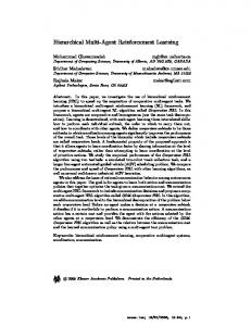
where r(s, a) is the reward for taking action a at state s, and v(s,*) is called optimal value for that state while P(s0|s, a) is the probability of transiting to state ′ After taking action an in state s. If the agent knows the reward and state transition functions, it can solve * by iterative search method, otherwise this method cannot be used while an algorithm called Q is employed [13] [14]. The variety of Q-functions has been used in [6,7,8,9,10]. Selfish Q-learning algorithm pseudo-code, which has been used in [7], is shown in Figure 1. In this algorithm, for every action a in each state S the value of that action (Q (s, a)) is used according to Equation 3. Each state S the value of that action (Q (s, a)) is used according to

Copyright (c) 2012 International Journal of Computer Science Issues. All Rights Reserved.

IJCSI International Journal of Computer Science Issues, Vol. 9, Issue 1, No 3, January 2012 ISSN (Online): 1694-0814 www.IJCSI.org

Equation 3. In Equation3, α is the rate of learning and γ  [0, 1] is the discount factor. The algorithm ends when the optimum policy doesn’t change for a definite while. ,



,

max

,

,

(3)

To select an action in every state, the Boltzmann’s distribution method (EQ 4) is usually used. This function has been used in some articles such as [6,7,8,9,10,19]. ,

arg max

π

(4) ,

∑

In which, m is the number of allowable actions for state S and is a constant. Q (S, a) shows the value of evaluation function of state S while action a is done. Algorithm Selfish Q‐Learning  1. Initialize Q(S,a) arbitrarily  2. Repeat (for each episode)  3. Initialize S randomly  4. Repeat (for each step)  5. Select an action using π

,

arg max ∑

,

6. Execute the action a  7. Observe reward r(s,a) ,state s’ 8. Update the value of Q(S,a) according to  max

,

,

 

  EQ(3)

 

 

 EQ(4)

,

,



9.  ← ′  10. Until S is Terminal State  11. Until some stopping Criteria is reached.  12. End      Fig 1. Selfish Q-Learning Algorithm

2.2. Markov Games Markov games are a generalization of MDPs to multiple agents and can be used as a framework for investigating multi-agent learning. In the general case (general-sum games), each player would have a separate payoffs. A standard formal definition follows: Definition 2. A stochastic game (Markov game) is a tuple n, S, A1..n, T, R1..n  , where n is the number of agents, s is a set of states, Ai is the set of actions available to agent i (and A is the joint action space A1× A2×. . . ×An ), T is a transition function S×A×S [0,1] ), and r is a reward function for the ith agent S×A. In a discounted Markov game, the objective of each player is to maximize the discounted sum of rewards, with a discount factor  [0,1). Let i be the strategy of the player i. For a given initial state s, player i tries to maximize:

∑

,

,

132

,…, | ,

(5) ,…,

,



Markov games are categorized based on the agent’s rewards into cooperative and non-cooperative games. Noncooperative games may be classified as competitive games and general-sum games. Strictly competitive games, or zero-sum games, are two-player games where one player’s reward is always the negative of the others. General-sum games are ones where the reward sum is not restricted to zero or any constant, and allow the agents’ rewards to be arbitrarily related. However, in full cooperative games, or team games, rewards are always positively related. In a fully cooperative MG (or team MG) called a multi-agent MDP (or MMDP), all agents share the same reward function. Nevertheless, in general MG (or general-sum MG) there is no constraint on the sum of the agents’ rewards and the agents should learn to find and agree on the same optimal policy. However, in a general Markov Game, an equilibrium point is sought; i.e. a situation in which no agent alone can change its policy to improve its reward when all other agents keep their policy fixed [15], [16]. One of the Markov’s games used for multi-agent Markov’s games is the Grid World game. In this game, two agents start from a corner of the page and try to reach a goal with the least possible number of moves. Players' actions are defined as four actions in four different directions, namely Up, Down, Left, Right. A state space set is defined , , In which each state s= , as | Indicates the coordinates of agents 1 and 2. Agents cannot take the same coordinates at the same time. In other words, if both agents try to move to the same square, both of their moves will fail. If agents move to two different non-goal positions, both receive zero rewards and if one reaches the goal position, it receives 100 units of reward. However, if they collide with each other both receive one unit of punishment and stay in their previous position. In this game, the state transition is deterministic, i.e. the next state is uniquely determined by the current state and the joint action of the agents. In this game, agents are assumed not to know the goal position and the other agent's reward functions. Agents choose their actions simultaneously and can only know about the previous moves of the other agents and their own current state. Another game which we have used it, called Tunnel to Goal. In this game, there are some barriers. If an agent collision these barriers, it receives one unit of punishment. A path in these games represents sequences of actions from the starting to the end position. In game terminology,

Copyright (c) 2012 International Journal of Computer Science Issues. All Rights Reserved.

IJCSI International Journal of Computer Science Issues, Vol. 9, Issue 1, No 3, January 2012 ISSN (Online): 1694-0814 www.IJCSI.org

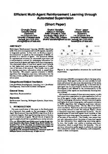
such a path is called a policy or strategy. The shortest path, not interfering the path taken by the other agent, is called the optimal policy or Nash path. Figure 2 is an example of these games. The optimal policy in Figure 2.a includes 9 movements and in Figure 2.b includes 10 movements.

(a) (b) Fig2 . examples of Markov Games. (2.a) An example of Grid World Game.

2.b. An example of Tunnel to Goal Game

2.3. Case Base Reasoning Case Based Reasoning (CBR) technique uses the previous experiences (Case) to solve the new problems [17], [18]. In the case base reasoning systems, the experiences gained from solving the problems are saved in case base (CB). In these systems, for solving the new problem (Cnew), the most similar cases to Cnew are extracted from the case base (CB) and the solutions presented by the extracted cases are used to solve the new problem C new. If a similar case is not found, Cnew is inserted is inserted to the case base as a new case. Unlike the classical knowledge-based methods, CBR focuses on a particular problem-solving experience, which is originated from the cases collected in the case base. These cases show a particular experience on a problem solving domain. It must be noted that CBR doesn’t recommend a definite solution, but presents hypothesis and theories pass the solution space.

133

algorithm with Selfish Q-Learning according to EQ(3) and called CB-BHASQL.

1

,

,

max

,

6

We know that solving a problem using CBR includes the steps: creating a description of the problem, evaluating the similarity of the current problem to the previously-solved problems saved in case base, and trying to reuse the solutions presented by the detected cases to solve the current problem. The structure of the cases used in the recommended algorithm is a duplex in the form of Case= in which, Prob describes the problem and Sol is the solution presented to solve the problem. The problem describer (Prob) includes the properties in each state. In the proposed algorithm, the problem describer is defined as Prob (S) = {m, , index} in which, m is the number of actions for each state and the set are the actions allowable for each action and index is the index for each state. The solution recommended for the problem is Sol (S) = , in which vector In the form of = ( [1], [2], …, [m]) is a list of experiences collected from the environment by the agent for state S and each vector includes a tuple where Ai is the space of actions for state S and Ni is the number of times that ai Ai has been updated and Qi is the value estimated by Equation 1 and πi is the possibility of occurrence of action ai , which is estimated by EQ(7). ,

π

arg max

∑

, ,

,



(7)

3. The Proposed method

Where m is the number of allowable actions for state S and n (S, a) is the number of times that so far the action a has been selected. Q (S, a) shows the value of evaluation function of state S while action a is done.

In this section, a new algorithm called CB-BHASQL is proposed to increase the rate of convergence in Markov’s games. In the proposed algorithm, the case base reasoning and also a new function are used to select the action in each state to increase the convergence rate toward the optimal policy. We previously used our new function with Decentralized Q-Learning according to EQ(6) and called CB-BHADQL. In this paper, We proposed a new

V is the justification of using the solution recommended by the detected agent and if each of the actions of state S at least has been selected once, the solution of the detected agent can be used for solving the new problem. In the recommended algorithm, once the agent enters a new state, extracts the most similar case to the new state of the case

Copyright (c) 2012 International Journal of Computer Science Issues. All Rights Reserved.

IJCSI International Journal of Computer Science Issues, Vol. 9, Issue 1, No 3, January 2012 ISSN (Online): 1694-0814 www.IJCSI.org

134

base and if the justification is available (V = True), the detected case is used to determine the next state.

CB-BHASQL algorithm has lower numbers of moves in comparison with the other algorithms.

To detect the similar cases of current state, the nearest neighbor algorithm is used. Euclidean distance of the new case to each of the cases available in case base is calculated according to EQ(8) and the most similar case (c) is detected and if the justification is available (V = True), the solution of detected case is used to solve the new problem. The proposed algorithm is shown in Figure 3.

Experiment 2. In this experiment, we compare the proposed algorithm (CB-BHASQL) in Grid World Games environment ( Fig 2.a) with the other algorithms in terms of the averaged reward received by agent 1during an episode. Figure 6 shows the result of this experiment. As it is seen (CB-BHASQL) algorithm outperforms the other algorithms in terms the average reward received during an episode.

arg arg

∈



.

∈

, .

. , .

(8)

Algorithm CB-BHASQL 1. Let t be the global time, n be the number of agents,



discount factor ,CBi= an empty case base for each Set

′

Repeat Set s=s’

4. Experiments

4.

forall agent

In order to evaluate the performance of the proposed algorithm several experiments have been conducted whose results are reported below. In Section 4.1, The environment of the experiments is a Grid-world game that includes a 5 6 Grid according to Figure 2.a. In section 4.2, the environment of the experiments is a Tunnel to Goal game that includes a 5 6 Grid according to Figure 2.b. These experiments are conducted to study the improvement obtained by the proposed algorithm (CBBHASQL) in comparison with three CBR and QL algorithms and CB-BHADQL. So, CB-BHASQL algorithm is compared with three algorithms: 1) Selfish QLearning algorithm, and 2) Boltzmann’s CBR algorithm, which its pseudo-code is similar to Figure 3 and the only difference is in the selection of the actions which is based on the Boltzmann’s distribution (Equation 4) and 3) CBBHADQL. In all experiments, each reported value is obtained by averaging over 200 runs and the average results are gained for the algorithms. Parameters given are = 0.05 and γ = 0.7.

5. 6. 7.

Experiment 1. In this experiment, we compare the proposed algorithm (CB-BHASQL) in Grid World Games environment ( Fig 2.a) with the other algorithms in terms of the number of movements made by agent 1 to reach the optimal path in 2000 episode. Figure 4 illustrates the results of this experiment. Figure 5 shows the average results after 200 runs. From the result, it is evident that the

i  [1...n] do

if CBi= or addcasecriterion(s) is true

CB  CB  C

with c.Prob=s and c.Sol=empty_solution (i)

for each j=Sol(s).m do

8.

Compute Sol(s).E[j].

i

according to EQ(7) and Set index

xi

the Maximum

value of them.

9.

Select elementary action

10. Observe Successor state 11. end if. 12. end for.

Sol ( s).E[ x i ].a i .

s' S

i  [1...n]

and reward

rR

.

do

13.

for all agents

14.

Retrieve nearest neighbour according to EQ(8) of state s’.

15.

Set Learning Rate

16.

Set

17.

i 

Sol ( s ).E[ x i ].Qi



max

Increment

1 1  Sol ( s).E[ xi ].ni

according to

,

,

Sol ( s ).E[ x i ].n i

,

,

EQ(3) .

by one.

18. Resort decremently the experience list Q in Sol(s).E 19. Until Stop_Criterion () becomes true. Fig 3. Pseudo-code for the Proposed Algorithm CB-BHASQL

CB‐BHADQL

Number of Movements

1000

In this section, we show results of our experiments in Grid word Games.

∈ to

the initial state of the system 2. 3.

4.1. Experiments in Grid World Games

the

Selfish Q‐Learning Boltzmann CBR

800

CB‐BHASQL

600 400 200 0 200

400

600

800

1000

1200

1400

1600

1800

2000

Episode

Fig4. Comparison of different methods in terms of the number of movements Needed for reaching to the optimal path in Grid World.

Copyright (c) 2012 International Journal of Computer Science Issues. All Rights Reserved.

IJCSI International Journal of Computer Science Issues, Vol. 9, Issue 1, No 3, January 2012 ISSN (Online): 1694-0814 www.IJCSI.org

135

CB‐BHADQL 200

500

Selfish Q‐Learning

400

Number of Movements

Average of Moves

CB‐BHASQL

150

CB‐BHADQL Selfish Q‐Learning Boltzmann CBR CB‐BHASQL

450

Boltzmann CBR

100

50

350 300 250 200 150 100 50

0 200

400

600

800

1000

1200

1400

1600

1800

0

2000

200

Episode

400

600

800

1000

1200

1400

1600

1800

2000

Episode

Fig5. Comparison of four Algorithms in terms of average of the number of moves to reaching optimal path in 200 runs in Grid World. 160

  Fig7. Comparison of different methods in terms of the number of movements Needed for reaching to the optimal path in Tunnel to Goal.

Average of Rewards

140

450

120

CB‐BHADQL Selfish Q‐Learning Boltzmann CBR CB‐BHASQL

400 350

80

300

60 40

CB‐BHADQL Selfish Q‐Learning Boltzmann CBR CB‐BHASQL

20 0 200

400

600

800

1000

1200

1400

1600

1800

Average of Moves

100

250 200 150 100

2000

50

Episode

0

Figure 6. Comparison of Three Algorithms in term of the average of rewards gained in 200 runs in Grid World.

200

400

600

800

1000

1200

1400

1600

1800

2000

Episode

Fig8. Comparison of four Algorithms in terms of average of the number of moves to reaching optimal path in 200 runs in Tunnel to Goal.

4.2. Experiments in Tunnel to Goal Games

Experiment 3. In this experiment, we compare the proposed algorithm (CB-BHASQL) in Tunnel to Goal Games environment ( Fig 2.b) with the other algorithms in terms of the number of movements made by agent 1 to reach the optimal path in 2000 episode. Figure 7 illustrates the results of this experiment. Figure 8 shows the average results after 200 runs. From the result, it is evident that the CB-BHASQL algorithm has lower numbers of moves in comparison with the other algorithms. Experiment 4. In this experiment, we compare the proposed algorithm (CB-BHASQL) in Tunnel to Goal Games environment ( Fig 2.b) with the other algorithms in terms of the averaged reward received by agent 1during an episode. Figure 9 shows the result of this experiment. As it is seen (CB-BHASQL) algorithm outperforms the other algorithms in terms the average reward received during an episode.

120

100 Average of Rewards

In this section, we show results of our experiments in Tunnel to Goal Games.

80

60

40 CB‐BHADQL Selfish Q‐Learning Boltzmann CBR CB‐BHASQL

20

0 200

400

600

800

1000 1200 Episode

1400

1600

1800

2000

Fig 9. Comparison of Three Algorithms in term of the average of rewards gained in 200 runs in Tunnel to Goal.

5. Evaluation of the Algorithm’s Behavior 5.1. Examination of the Behavior of the Proposed Algorithms In this section, an analysis of the performance the proposed algorithm is conducted in which the advantage of the function π2 (S) (EQ 7) is compared with π1 (S) (EQ 4). We want to show that in the proposed method, π2 (S) in comparison with π1 (S) converges to the optimum solution with a higher rate. In other words, the rate of variation for

Copyright (c) 2012 International Journal of Computer Science Issues. All Rights Reserved.

IJCSI International Journal of Computer Science Issues, Vol. 9, Issue 1, No 3, January 2012 ISSN (Online): 1694-0814 www.IJCSI.org

Experiment 5. In this experiment, variations of π2 (S) were evaluated in comparison with π1 (S). Figures 10-12 show these variations As it is seen, we note that regarding to the increase in n, the growth of π2 (S) is much more than π1 (S). Experiment 6. In this experiment, we study evaluation of variations for function Q (S, a) (EQ(3)) regarding to the increase in n. The results of this analysis are shown in Figures 11-13. As it is seen, we conclude that with increasing n, the value of function Q (S, a) also increases in Equation 3. Experiment 7. In this experiment, we study evaluation of variations for π1 (S) and π2 (S) based on values for Q (S, a). The results of this evaluation are shown in Figure 14. Looking at the diagram we note that with increasing value of Q (S, a), the value of π1 (S) increases. Since always limt→∞ not (S, a) = ∞, according to the result of Experiment 6, value of Qt (S, a) increases and according to the result of Experiment 6, with increasing n, the function π2 (S) grows faster than π1 (S). Based on the previous subjects, it is concluded that with increasing value of Qt (S, a), the function π2 (S) must grow faster than π1 (S). Figure 15 shows the results.

(12) Through the comparison of the EQ(11) and EQ(12), we conclude that the growth of the rate Is less

than

.

In Equation 11, because Q is positive, the value of function is always positive. According to equation 3 and the diagram in Figure 11, with increasing n, the value of Q (S, a) always increases. Thus, > 0 and from

the other hand, n> 0 and Q> 0. So,

is always

positive. is multiplied by the constant value In Equation 10, is multiplied by 20. This is while in Equation 12, variant Q. With increasing n, the value of Q increases. is less than . The Thus, the growth rate of diagram in Figure 15 also supports the result gained.

10

1(S0,a1) 2(S0,a1)

9 8 7

(S0,a1)

π2 (S) in relation to Q, is more than the rate of variation for π1 (S) in relation to Q. To show the advantage of the behavior of the proposed action selection function, the CB-BHASQL algorithm was evaluated for state S0 and action a1 regarding to different values of n and the results below were gained:

136

6 5 4 3 2 1 0

To facilitate the calculations, we rewrite functions π1 (S) and π2 (S) as EQ (9) and EQ (10) respectively.

(9) ∑



(10)

0

5

10

15

20

25

n(S0,a1)

Fig 10. Examining the growth of π2 (S) and π1 (S) based on the different n values

30

n(S0,a1)

5.2. Mathematical Analysis of the Functions Behavior

20

10

0 0 0.5

The variable rate of π1 (S) in relation to Q with parameter t = 0.05, is shown in EQ (11). .

.

20



(11)

1 1.5 14

x 10

 2(S0,a1)

2

0

0.5

1

2

1.5

2.5

3

3.5

4

4.5

Q(S0,a1)

Fig 11. Examination of π2(S) variations based on the different n values.

The variable rate of π1 (S) in relation to Q is shown in EQ ( 12).

Copyright (c) 2012 International Journal of Computer Science Issues. All Rights Reserved.

n(S0,a1)

IJCSI International Journal of Computer Science Issues, Vol. 9, Issue 1, No 3, January 2012 ISSN (Online): 1694-0814 www.IJCSI.org

new function has been applied to select the action in each state. The results gained were compared with the current algorithms. Based on the results gained in two different environments, in comparison with Selfish Q-Learning and Boltzmann’s CBR algorithms and CB-BHADQL, our proposed algorithm CB-BHASQL algorithm has a very high efficiency from the perspective of convergence rate to the optimum answer, average of total reward gained and the number of the movements needed for convergence to the optimal policy.

30 20 10 0 0.5 0.6 0.7 0.8 0.9 1

1

0.5

0

2

1.5

2.5

3

3.5

4.5

4

Q(S0,a1)

1(S0,a1)

137

Fig 12. Examination of π1 (S) Variations based on the Different n values. 4.5

References

4

Q(S0,a1)

3.5 3 2.5 2 1.5 1 0.5 0

0

5

10

15

20

25

30

n(t) Fig 13. Examination of Q (S, a) Variations based on the Different n values. 1 0.95

1(S0,a1)

0.9 0.85 0.8 0.75 0.7 0.65 0.6 0.55 0.5

0

0.5

1

1.5

2

2.5

3

3.5

4

4.5

Q(S0,a1)

Fig 14. Examination of π1 (S) Growth based on the Different Q (S, a) values. 10

1(S0,a1)

9

2(S0,a1)

8

 (S0,a1)

7 6 5 4 3 2 1 0

0

0.2

0.4

0.6

0.8

1

1.2

1.4

1.6

1.8

2

Q(S0,a1) Fig 15. Examination of π1 (S) and π2 (S) Growth based on the Different Q (S, a) values

6. Conclusion In this paper, a new hybrid model called CB-BHAQL has been introduced to solve Markov’s games based on reinforcement learning and case base systems, in which a

[1] R. A. C. Branchi, R. Raquel, R. L. D. Mantaras, ” Imroving Reinforcement Learning by using Case Based Heuristics”, Proceeding of the Int. Conference on Case Based Learning 2009 (ICCBR 2009), Springer , 2009. [2] N. Vlassis, “A Concise Introduction to Multiagent Systems and Distributed Artificial Intelligence”, 2007, Morgan and Claypool Publishers. [3] C. Boutilier, "Sequential optimality and coordination in multi-agent systems", in: Proceedings of the 16th International joint conference on Artificial intelligence, 1999 , Vol. 1, Morgan Kaufmann Publishers Inc., Stockholm, Sweden. [4] L. Bosniu, R. Babuska, and B. Schutter, "A Comprehensive Survey of Multiagent Reinforcement Learning", IEEE Transaction on System, Man, Cybern, 2008 ,vol. 38, pp. 156171. [5] B. Masoumi, M. R. Meybodi, “Speeding up learning automata based multi agent systems using the concepts of stigmergy and entropy”, Journal of Expert Systems with Applications, July 2011, Vol 38, Issue 7, PP. 8105-8118. [6] M. Lauer and M. Riedmiller, "An Algorithm for Distributed Reinforcement Learning in Cooperative Multi-Agent Systems", in The 17th International Conference on Machine Learning San Francisco, CA, USA, 2000: Morgan Kaufmann Publishers Inc, pp. 535 – 542. [7] A. G. Barto and R. S. Sutton, “Reinforcement Learning: an introduction”, MIT Press, Cambridge, MA, 1998. [8] X. Wang and T. Sandholm, "Reinforcement Learning to Play an Optimal Nash Equilibrium in Team Markov Games", in Advances in Neural Information Processing Systems, 2002, vol. 15: MIT Press, pp. 1571-1578, 2002, [9] F. S. Melo, M. I. Ribeiro, “Reinforcement Learning with Function Approximation for Cooperative Navigation Tasks”, IEEE International Conference on Robotics and A Utomation Pasadena, CA, USA, May 2008, pp. 3321-2237. [10] M. Lauer and M. Riedmiller, “Reinforcement Learning for Stochastic cooperative Multi-agent Systems”, In Proceeding of AAMAS 2004, New York, NY, ACM Press, pp. 15141515. [11] R. A. C. Bianchi, C. H. C. Ribeiro, A. H. R. Costa, “ Accelerating autonomous learning by using a heuristic selection of actions”, Journal of Heuristis , , 2008, Vol. 2, pp.135-168. [12] R. A. C. Bianchi, C. H. C. Ribeiro, A. H. R. Costa, ”Heuristic selection of actions in multi agent reinforcement

Copyright (c) 2012 International Journal of Computer Science Issues. All Rights Reserved.

IJCSI International Journal of Computer Science Issues, Vol. 9, Issue 1, No 3, January 2012 ISSN (Online): 1694-0814 www.IJCSI.org

learning”, 20th International conference on Artificial Intelligence, India , Jan 2007, pp.690-695. [13] L. Puterman, Markov Decision Processes: Discrete Stochastic Dynamic Programming, John Wiley and Sons, New York, 1994. [14] R. S. Sutton, A. G. Barto, “Reinforcement Learning : An Introduction”, MIT Press, 1998. [15] J. F. Nash, “Non-cooperative Games”, Annals of Mathematics, , 1951, Vol. 54, pp. 286–295. [16] A. M. Fink, Equilibrium in a Stochastic N-person Game, Journal of Science in Hiroshima University, Series A-I, 1964, Vol. 28, pp. 89–93. [17] A. Aamodt; E. Plaza, "Case-Based Reasoning: Foundational Issues", Methodological Variations and System Approaches AI Communications, IOS Press, 1994, Vol. 7, No. 1, pp. 39-59. [18] R. Bergman; "Engineering Applications of Case Based Reasoning", Journal of Engineering Applications of Artificial Intelligence, 1999 , Vol. 12, pp.805. [19] Gabel, T. And Riedmiller, M., “CBR for state value function Approximation in Reinforcement Learning”, Proceeding of the Inter. Conference on Case Based Learning 2005 (ICCBR 2005) , Springer , Chicago, USA.

Sara Esfandiari received her BS degree in Computer Engineering from the azad University, Tehran, Iran., in 2006 and MS degree in Computer Engineering in 2011 from the azad University, Qazvin, Iran. Her research interests include Learning systems, multi agent systems, multi agent learning, Data Mining, parallel algorithms. Behrooz Masoumi received his BS and MS degrees in Computer Engineering in 1995 and 1998, respectively. He also received his PhD degrees in Computer Engineering from the Science and Research University, Tehran, Iran., in 2011. He joined the faculty of Computer and IT Engineering Department at Qazvin Azad University, Qazvin, Iran, in 1998. His research interests include learning systems, multi-agent systems, multi-agent learning, and soft computing. Mohammadreza Meybodi received his BS and MS degrees in Economics from the Shahid Beheshti University in Iran, in 1973 and 1977, respectively. He also received his MS and PhD degrees in Computer Science from the Oklahoma University, U.S.A., in 1980 and 1983, respectively. Currently he is a Full Professor in the Computer Engineering Department, Amirkabir University of Technology, Tehran, Iran. Prior to his current position, he worked from 1983 to 1985 as an Assistant Professor at Western Michigan University, and from 1985 to 1991 as an Associate Professor at Ohio University, U.S.A. His research interests include channel management in cellular networks, learning systems, parallel algorithms, soft computing, and software development. Abdolkarim Niazi is currently PhD Student in Mechanical Engineering-Manufacturing engineering at Technical University of Malaysia from 2010 up to now. His research interests include Condition monitoring, Tools Condition monitoring, Tool wear and tool vibration, Advance and Automated Manufacturing Systems, Artificial Neural Networks.

Copyright (c) 2012 International Journal of Computer Science Issues. All Rights Reserved.

138