Improving Music Information Retrieval using Segmentation-related Statistics Stephen Travis Pope FASTLab, Inc., Santa Barbara, California, USA
[email protected]
ABSTRACT The next generation of music databases will be required to search on musical genre, mood, song style and user preference. For this, we need analyzer programs that create song feature vectors in a multi-stage process of signal processing, data smoothing and statistics, and song segmentation. This paper discusses the high-level features that can be derived from music segmentation, i.e., finding the breakpoints between the musical verses and choruses. We address segmentation and related statistics, and present a software implementation and test data for discussion and evaluation.
Keywords Music information retrieval, multimedia databases, audio analysis, music segmentation, data-mining, machine-learning
1.
INTRODUCTION
Music information retrieval (MIR) software uses signal analysis for feature extraction from song data in applications such as genre/mood classification, finger-printing, thumbnailing and playlist generation (recommendation). MIR analyzers perform detailed signal analysis and post-analysis data processing and statistics, creating feature vectors with a variety of time- and frequency-domain fields [5]. This paper describes the use of a music segmenter to deliver a set of database features that improve the quality of MIR applications. A number of high-level statistics are gathered based on the output of the song segmenter, and these prove useful in a variety of data-mining and machine learning algorithms and a playlist-generation application. We introduce music segmenters and then the array of segmentation-derived features that can be added to the feature vector. Results are evaluated of the role that these new features play in tasks like principal component analysis, rule-learning, and similarity metrics. The MIR song analysis process consists of a windowed feature extraction stage that reads audio data and performs signal analysis routines on short windows (1-50 msec = 64-2000
Permission to make digital or hard copies of all or part of this work for personal or classroom use is granted without fee provided that copies are not made or distributed for profit or commercial advantage and that copies bear this notice and the full citation on the first page. To copy otherwise, to republish, to post on servers or to redistribute to lists, requires prior specific permission and/or a fee. MAST ’09, Santa Barbara, California USA, January, 2009 Copyright 200X ACM X-XXXXX-XX-X/XX/XX ...$5.00.
samples), yielding a set of raw time- and frequency-domain (and other) features. The second-pass analysis smoothes the raw data and derives higher-level features (e.g., tempo or spectral tracks), followed by pruning and reduction based on numerical/statistical analysis such as histograms or Gaussian mixture models. The third (application-specific) stage involves machine-learning or data-mining techniques such as clustering, classification or structure-learning [5]. In the early years of MIR (1985-95), research concentrated on rudimentary time- and frequency-domain features such as (1) windowed amplitude data and derived tempo statistics, and (2) windowed spectra, reduced spectra, and derived spectral statistics (”spectral measures”). The next generation of MIR (roughly 1995-2005), saw the introduction of more sophisticated features involving higher-level time- and frequency-domain features such as beat histograms, Melfrequency cepstral coefficients (MFCCs) and chromagrams. In addition, researchers began using more sophisticated statistics to aggregate the values of each feature within a song, and using newer machine-learning techniques.
2.
MUSIC SEGMENTATION
Automatic music segmentation means finding the breakpoints between the verses and choruses of a song (or the structural segments of a classical composition). For a pop song with clear instrumental breaks, or a jazz piece with tempo changes at the start of each solo, a segmenter would simply have to collect the feature vector data, and look for regularly spaced peaks in the weighted distance between windows. In fact, for many simple cases, this technique is sufficient to locate segment boundaries, and successful segmentation systems have been reported [1, 6]. As an example, look at the inter-window distance data shown in Figure 1, which displays the data for five different feature weightings for a one-minute excerpt of a pop song. One can easily see the similarities and also the differences both in average value and in dynamic range; most observers would say that there are five (or so) ”periods” or phrases in the portion of the graph shown here. Examples of the feature weightings used are given in the Appendix. Figure 2 shows the auto-correlation of the distance data for several of these feature weightings; the lower values on the left are the short-time regularities (beats), and the higher peaks on the right correspond to the phrases and verses. Again one can observe clear similarities in the auto-correlation peaks with different feature weightings, with significant differences in data offset and dynamic range among them. Finding a musically relevant segmentation means using
tion include tempo changes, intro/outro sections, click-track tempo, and songs with very compressed dynamic range.
3.
Figure 1: Inter-window distances using five different feature weightings over 1 minute of a song
Figure 2: Auto-correlation of the windowed distance function for several of the feature weightings distance metrics and inter-segment-boundary detection and working either bottom-up (grouping short segments into subsets of the song) or top-down (dividing the song into a string of segments) to pick a song segmentation expressed as a list of ”verse/chorus” break-points. Our approach [4] is to find the peaks in the inter-window distance function, build a tree of them based on the expected repetition of short segments, and find the best matches for the song. We start by creating the peak-index list from a distance function, and guess at a peak period (segment length) from the function’s auto-correlation for which to search. We traverse the peak-index list looking for peaks with a periodicity at the selected period; if we find a strong periodicity (regularly spaced distance function peaks over a long interval), we nominate the chosen peak and period as a part of a segmentation candidate. We can quickly generate a list of proposed segmentations based on different starting peaks and periods, and combine these to cover the song. To evaluate a collection of proposed segmentations, a polynomial confidence value is computed based on factors such as: * * * * * *
# of segments per song (2-8 preferred) % of song accounted for (aside from intro/outro) % of peaks accounted for (% off-beats) # of peaks per segment (hope for many) Which weighting was used (prefer broad weightings?) Peak-match tolerance (prefer stricter timing?)
In our experience, small changes in this weighting influence the segmenter success rate, but the cases of having too many segments (i.e., finding 2-bar sections rather than whole verses) or too few (1st-half/2nd-half), can both be controlled. For complex music, or heavily compressed productions (either in the sense of dynamic range compression in post-production, or of lossy compressed encoding), segmentation techniques are required that incorporate an adaptive distance weighting and/or a multi-pass distance peak-finding algorithm. The specific challenges to segmenta-
SEGMENTATION-DERIVED FEATURES
Assuming a segmenter with a high confidence for the majority of songs in a database, the question arises of what new high-level features can be derived from the segmentation data to assist specific applications. The output of the segmenter will be represented as a list of segment breakpoints; from this data, we can derive a whole array of related (and semantically relevant) musical features, although the segmentation itself is all that’s required for some applications (e.g., thumb-nailing or summarization). First, we look at the first and last regions (whether they’re in-segment or not) and see if they look like fade-in or fadeout sections, or more like contrasting intro or ”outro” sections for the song (coda, repeat of the chorus, etc.). Next, we compute the per-segment averaged (or mean value) feature vectors and try to identify the ”typical” and ”solo” segments, i.e., the most average-sounding segment that starts at a regular period, and the segment at the same period that’s most different and is not the intro/outro section. If we succeed at finding these, we create a new set of segmentation features based on the ratios of selected features between the ”typical” and the ”solo” segments. A third statistic of interest is the segment-level dynamic range, expressed as the percentage of segments that are significantly louder or quieter than the typical segment. The solo/verse segment data can be used to select short sections (e.g., 1 beat or 1 second) for detailed analysis, for example to identify the main voice(s) or the spectral signature of the solo instrument. The segmentation data is useful for pruning the main song feature vector, summing the core features over the chosen verse (or just a few seconds of it), and storing the mean and variance (or GMM or histogram) for each feature. We are exploring other segmentation-derived features; this list represents the current feature set. Collecting the outputs of the segmenter and the derived features together, we have: * * * * * * * * *
Segmenter confidence (range 0 - 1; value < 0.2 —> ignore) Number of segments (2 - 16 in normal music) Verse length (10 - 60 seconds) First verse start (length of intro/prelude) Typical/Solo start (start of the verse/solo section) Typical/Solo index (1-16, rarely 1 or 16) Quiet/Loud sections (% of quiet/loud sections) Fade-In/Out (# secs to reach avg. amplitude) Solo/Verse ratios: RMS, Tempo, SpectralCentroid, SpectralVariety, DynamicRange (more possible here)
As an example of a successful segmentation, the text below is the output of a database query for some of the segmenter features of a pop/dance song that segmented well (numerical features are normalized to the range 0-1). Database fields: | title | segmentweight | numsegments | I Believe In Love | 0.923772 | 0.24 | verselength | typicalstart | solostart | 0.631119 | 0.280232 | 0.590672 | s_centroid | s_variety | s_tempo | s_dynrange | 0.4991 | 0.001422 | 0.3360 | 0.654455
Note first that the confidence (segmentweight) is high (0.924); the numsegments of 0.24 corresponds to 7 segments (normalized to a maximum of 30 per track). The verselength (0.63, normalized to 0-30 seconds), typicalstart (0.28 of the way through the song), and solostart (0.59 of the way through the song) values are each correct. The solo/verse ratio features (s centroid, s variety, s tempo, s dynrange and especially the s variety, the solo-verse spectral variety ratio) are all quite low because this song has an acoustic piano as the solo instrument, i.e., it’s much ”darker,” less dynamic in timbre, and perceptually ”slower” than the vocal verses.
4.
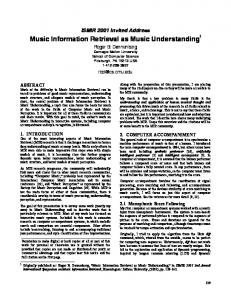
Figure 3: PCA dimension weights for simple (FV1) and extended (FV2, FV3) feature vectors showing the contribution of the new segmentation-derived features to the decomposition.
EVALUATION AND DISCUSSION
An analyzer for this feature vector has been implemented over several generations in the form of the Music Analysis Kernel (MAK) in C++, Smalltalk, MATLAB and SQL [3, 4]. The MAK feature vector incorporates a rich set of time- and frequency-domain features and uses segmentationinformed statistics to store a single song-typical mean and variance value for each of the 26-40 core features (listed in the Appendix). A multi-output tempo estimator delivers tempo-related features alongside a bass pitch follower and key/chroma analysis. Beyond this, we store several beat histogram features [6], including the low/high peak amplitudes, BPM tempi and octave sums. We add the fluctuationpattern (FP) measures fp gravity, fp bass and fp focus [2], and the set of 17-20 segmentation features introduced above. The segmenter is a multi-weighting, multi-tolerance peaktree blackboard algorithm with the complex confidence measure given above; for our (eclectic) test set of 15000 songs, allowing up to 16 segments per song, it fails about 3% of the time (about equal to the ratio of spoken-word content in the test set). If we reduce the limit to 12 segments per song, the failure rate only rises to 7%. How can we quantify the contribution of the new features in real-world applications (their ”applied information gain” as it were)? We turn to dimensionality reduction, information theory and data mining techniques, and start with the principal component analysis (PCA) of the song data, which delivers polynomial equations that describe the dimensions of decomposition (the principal components) of the data set. The quality of the analysis is reflected in the number of components whose weight exceeds a given threshold. To test this, we ”prune” the data and repeat PCA decomposition with three subsets of the feature vector: * FV1 = 26 base-features and their variances * FV2 = FV1 + beat histogram and flux-patterns * FV3 = FV2 + 17 segmentation-derived features
Figure 3 shows the weights of the PCA dimensions contributing more than a threshold of 0.09. For FV1 (left-most and lowest data series), we see that only 9 PCA dimensions were identified, while FV2 (adding the advanced features), gave us both higher PCA dimension weights and more of them (16). For the vector that includes the segmentation features (FV3), we observe both higher values and more dimensions (26) for the PCA processing. If we look at the actual PCA equations (listed in the Appendix), we see that the first dimension consists exclusively of high-level spectral variables (spectral measures, MFCC, spectral tracker data and their variances), while dimension two is a mix of fluctuation pattern. beat histogram, tempo,
segmentation, and solo ratio features (SegmentWeight, QuietSections, SoloStart, SoloTempo, FadeIn and LoudSections). The third dimension combines a different set of segmentation data (VerseLength, QuietSections, LoudSections and FadeOut). The next three PCA dimensions each incorporate significant contributions from different combinations of the segmentation-derived features (in consort with fluctuation pattern, beat histogram and tempo features, and variances of the MFCC data and spectral measures). This is very encouraging. As another test, we derive PART decision lists, a datamining technique that ”discovers” weighted rules describing the data set; for our test data, the segmentation features play a role in many PART rules, such as, ZeroCrossingsVar 0.2) -- # segments -- verse length in sec -- start of 1st main section -- start time of the verse and solo -- start time of the verse and solo
FadeIn real, FadeOut real,
-- fade in/out times
QuietSections real, LoudSections real,
-- ratio of quiet/loud sections
SoloCentroid real, -- ratios of the spectral content of solo vs verse SoloVariety real, SoloDynRange real, SoloTempo real, -- ratios of the tempo/RMS of solo vs verse SoloRMS real, -- Clusterer features follow );
7.2
Feature Weightings for Distance Functions
Several parts of the analyzer offer the user the chance to alter their behavior by providing a feature weighting that is used to derive an inter-window distance measure. These are given in a configuration file and are called SegmenterConfiguration, ClustererConfiguration, DistanceConfiguration, and PCAConfiguration; they are each simple lists of features and associated weights (on an arbitrary scale). Two simple examples are given below. (It still requires recompilation to switch the actual distance metric, e.g., to change from a Euclidean space to using earth-mover’s distance [which is the default at present] or a Mahanalobis metric.) # Segmenter Configurations # Each block consists of a list of distance-metric # weighting maps keyed by feature # Spectral-/pitch-centric configuration SegmenterConfiguration { HPRMS 0.5 DynamicRange 0.5 ZeroCrossings 0.5 BassPitch 0.5 SpectralSlope 1 SpectralCentroid 1 SpectralVariety 1 SpectralBandMax 1 } # MFCC- & tracking-centric configuration SegmenterConfiguration { HPRMS 0.2 SpectralVariety 1 ZeroCrossings 0.2 BassPitch 0.5 STrackBirths 0.5 STrackDeaths 0.5 MFCCCoeff1 1 MFCCCoeff2 1 MFCCCoeff3 1 MFCCCoeff4 1 MFCCCoeff5 1 MFCCCoeff6 1 }
7.3
PCA Dimensions
We present here the polynomial weightings for the first five dimensions of the principal components decomposition of our test database of 15000 songs. We have emphasized the contribution of the segmentation features. 1 0.18 MFCCCoeff6 + 0.18 MFCCCoeff5 + 0.18 MFCCCoeff4 + 0.18 MFCCCoeff3 + 0.18 MFCCCoeff2 + 0.18 SpectralFlux + 0.18 SpectralRolloff + 0.18 SpectralFluxVar + 0.18 SpectralSlopeVar + 0.18 SpectralRolloffVar + 0.18 SpectralSlope + 0.18 MFCCCoeff6Var + 0.18 MFCCCoeff5Var + 0.18 MFCCCoeff4Var + 0.18 MFCCCoeff3Var + 0.18 MFCCCoeff2Var + 0.179 SpectralBand2Var + 0.179 SpectralBand1Var + 0.179 STrackDeathsVar + 0.179 SpectralBand4Var + 0.179 STrackBirthsVar + 0.179 SpectralBand3Var + 0.179 SpectralBand3 + 0.179 SpectralBand2 + 0.179 STrackDeaths + 0.179 STrackBirths + 0.179 SpectralBand4 + 0.179 SpectralBand1 + 0.168 SpectralBandMax + 0.161 MFCCCoeff1 + 0.151 SpectralBandMaxVar + 0.097 SpectralCentroidVar 2 0.379 BHSUM3 - 0.345 LowPeakAmp - 0.322 BHSUM1 - 0.309 BHSUM2 - 0.298 HighPeakAmp - 0.294 fp bass - 0.268 ZeroCrossingsVar - 0.26 ZeroCrossings - 0.231 HPRMS + 0.162 TempoWeight + 0.162 TempoAvg - 0.155 fp gravity + 0.125 fp focus + 0.113 HighPeakBPM - 0.104 LPRMSVar + 0.093 LowPeakBPM + 0.08 HPRMSVar - 0.072 SpectralVarietyVar - 0.06 SegmentWeight + 0.054 QuietSections - 0.053 DynamicRangeVar 0.052 SpectralVariety + 0.048 SoloStart - 0.046 SpectralBandMaxVar - 0.044 RMSVar - 0.041 PeakVar - 0.039 SoloTempo + 0.035 FadeIn + 0.034 LoudSections + 0.033 HighLowRatio + 0.032 SpectralCentroidVar - 0.031 MFCCCoeff1Var 3 0.388 PeakVar + 0.365 RMSVar - 0.29 SpectralVariety + 0.284 HPRMSVar - 0.28 HPRMS - 0.234 ZeroCrossings - 0.225 SpectralVarietyVar - 0.193 fp gravity + 0.184 MFCCCoeff1Var + 0.183 fp bass - 0.15 MFCCCoeff1 + 0.149 fp focus + 0.138 LPRMSVar + 0.136 DynamicRangeVar + 0.135 VerseLength + 0.125 HighPeakAmp + 0.12 BHSUM2 + 0.114 QuietSections + 0.112 BHSUM3 - 0.111 ZeroCrossingsVar + 0.11 LowPeakAmp + 0.109 SpectralCentroidVar + 0.098 BHSUM1 + 0.095 SpectralCentroid + 0.075 DynamicRange + 0.074 LoudSections + 0.066 FadeOut + 0.066 LowPeakBPM + 0.062 BassDynamicityVAR + 0.061 TempoAvg - 0.059 NumSegments + 0.057 HighPeakBPM 4 0.432 DynamicRange + 0.404 DynamicRangeVar + 0.334 SpectralVarietyVar + 0.316 SpectralVariety - 0.272 LPRMSVar - 0.237 ZeroCrossings - 0.222 HPRMS - 0.205 fp focus + 0.203 HPRMSVar + 0.162 TypicalStart + 0.131 SegmentWeight + 0.129 SoloTempo + 0.116 VerseLength + 0.106 fp gravity + 0.105 SoloDynRange + 0.101 MFCCCoeff1 - 0.1 ZeroCrossingsVar - 0.088 LoudSections + 0.087 FadeOut + 0.078 FadeIn - 0.077 SpectralBandMaxVar - 0.076 TempoAvg - 0.055 RMSVar - 0.054 SpectralCentroidVar + 0.054 BHSUM3 + 0.052 BHSUM2 + 0.042 NumSegments - 0.039 MFCCCoeff1Var + 0.037 LowPeakAmp - 0.036 SpectralCentroid + 0.036 HighPeakBPM - 0.034 TempoWeight 5 0.463 TypicalStart + 0.457 SoloTempo + 0.441 NumSegments + 0.353 SoloStart - 0.286 TempoAvg + 0.196 LowPeakBPM + 0.171 HighPeakBPM - 0.122 DynamicRangeVar - 0.103 DynamicRange - 0.085 SoloRMS - 0.081 SegmentWeight + 0.081 FadeOut + 0.081 fp gravity - 0.078 TempoWeight + 0.075 FadeIn - 0.073 HPRMSVar - 0.072 SpectralVariety + 0.068 SpectralCentroid - 0.067 SpectralVarietyVar - 0.059 HighLowRatio + 0.056 MFCCCoeff1Var + 0.05 SpectralCentroidVar + 0.046 LoudSections + 0.039 ZeroCrossings - 0.038 fp bass + 0.036 BHSUM2 - 0.035 MFCCCoeff1 - 0.032 BHSUM1 + 0.032 SoloCentroid + 0.029 fp focus + 0.027 BassDynamicity - 0.027 RMSVar