Improving Named Entity Disambiguation by ... - Semantic Scholar

Improving Named Entity Disambiguation by Iteratively Enhancing Certainty of Extraction Mena B. Habib and Maurice van Keulen Faculty of EEMCS, University of Twente, Enschede, The Netherlands

{m.b.habib,m.vankeulen}@ewi.utwente.nl

ABSTRACT Named entity extraction and disambiguation have received much attention in recent years. Typical fields addressing these topics are information retrieval, natural language processing, and semantic web. This paper addresses two problems with named entity extraction and disambiguation. First, almost no existing works examine the extraction and disambiguation interdependency. Second, existing disambiguation techniques mostly take as input extracted named entities without considering the uncertainty and imperfection of the extraction process. It is the aim of this paper to investigate both avenues and to show that explicit handling of the uncertainty of annotation has much potential for making both extraction and disambiguation more robust. We conducted experiments with a set of holiday home descriptions with the aim to extract and disambiguate toponyms as a representative example of named entities. We show that the effectiveness of extraction influences the effectiveness of disambiguation, and reciprocally, how retraining the extraction models with information automatically derived from the disambiguation results, improves the extraction models. This mutual reinforcement is shown to even have an effect after several iterations.

Categories and Subject Descriptors

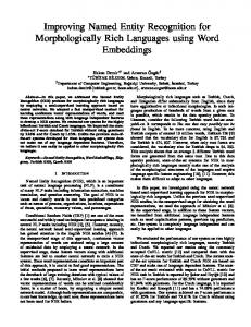
4 or more references 29% 1 reference 54% 3 references 5%

12% 2 references

Figure 1: Toponym ambiguity in GeoNames: top10, long tail, and reference frequency distribution.

I.7 [Document and Text Processing]: Miscellaneous

General Terms Algorithms

Keywords Named Entity Extraction, Named Entity Disambiguation, Uncertain Annotations.

1.

INTRODUCTION

Named entities are atomic elements in text belonging to predefined categories such as the names of persons, organiza-

tions, locations, expressions of times, quantities, monetary values, percentages, etc. Named entity extraction (a.k.a. named entity recognition) is a subtask of information extraction that seeks to locate and classify those elements in text. This process has become a basic step of many systems like Information Retrieval (IR), Question Answering (QA), and systems combining these, such as [1]. One major type of named entities is the toponym. In natural language, toponyms are names used to refer to locations without having to mention the actual geographic coordinates. The process of toponym extraction (a.k.a. toponym recognition) is a subtask of information extraction that aims to identify location names in natural text. The extraction techniques fall into two categories: rule-based or based on supervised-learning. Toponym disambiguation (a.k.a. toponym resolution) is the task of determining which real location is referred to by a certain instance of a name. Toponyms, as with named entities in general, are highly ambiguous. For example, accord-

ing to GeoNames1 , the toponym “Paris” refers to more than sixty different geographic places around the world besides the capital of France. Figure 1 shows the top ten of the most ambiguous geographic names. It also shows the long tail distribution of toponym ambiguity and the percentage of geographic names with multiple references. Another source of ambiguousness is that some toponyms are common English words. Table 1 shows a sample of Englishwords-like toponyms along with the number of references they have in the GeoNames gazetteer. This problem makes toponym extraction, by just matching text tokens against a gazetteer, an ineffective approach. And General In A

2 3 11 16

The All You As

3 3 11 84

be ‘all-or-nothing’. In other words, all steps, including entity recognition, should produce possible alternatives with associated likelihoods and dependencies. Our Contributions. In this paper, we focus on this principle. We turned to statistical approaches for toponym extraction. The advantage of statistical techniques for extraction is that they provide alternatives for annotations along with confidence probabilities. Instead of discarding these, as is commonly done by selecting the top-most likely candidate for further processing, we use them to enrich the knowledge for disambiguation. The probabilities proved to be useful in enhancing the disambiguation process. We believe that there is much potential in making the inherent uncertainty in information extraction explicit in this way. For example, phrases like “Lake Como” and “Como” can be both extracted with different confidence probabilities. This restricts the negative effect of differences in naming conventions of the gazetteer on the disambiguation process.

Table 1: A Sample of English-words-like toponyms In natural language, humans rely on the context to disambiguate a toponym. Context is also used in auomatic toponym disambiguation techniques. Existing techniques for toponym disambiguation can be classified into three categories: map-based, knowledge-based, and data-driven or supervised. A general principle in Direct effect our work is our be$ lief that named entity Toponym Toponym extraction and disamDisambiguation Extraction d biguation are highly dependent. In previReinforcement effect ous work [2], we studied not only the posFigure 2: The reinforceitive and negative efment effect between the tofect of the extraction ponym extraction and disprocess on the disamambiguation processes. biguation process, but also the potential of using the result of disambiguation to improve extraction. We called this potential for mutual improvement, the reinforcement effect (see Figure 2). To examine the reinforcement effect, we conducted experiments on a collection of holiday home descriptions from the EuroCottage2 portal. These descriptions contain general information about the holiday home including its location and its neighborhood (See Figure 4 for an example). As a representative example of toponym extraction and disambiguation, we focused on the task of extracting toponyms from the description and using them to infer the country where the holiday property is located. Section 3 presents a summary of the result analysis, observations, and thoughts of [2]. In general, we concluded that many of the observed problems are caused by an improper treatment of the inherent ambiguities. Natural language has the innate property that it is multiply interpretable. Therefore, none of the processes in information extraction should 1 2

www.geonames.org http://www.eurocottage.com

Second, extraction models are inherently imperfect and generate imprecise confidence probabilities for extraction. We were able to use the disambiguation result to enhance the confidence of true toponyms and reduce the confidence of false positives. This enhancement of extraction improves as a consequence the disambiguation (the aforementioned reinforcement effect). This process can be repeated iteratively as long as there is improvement in the extraction and disambiguation. Paper Organization. The rest of the paper is organized as follows. Section 2 presents related work on named entity extraction and disambiguation. Section 3 presents a problem analysis and our general approach to iterative improvement of toponym extraction and disambiguation based on uncertain annotations. The adaptations we made to toponym extraction and disambiguation techniques are described in Section 4. In Section 5, we describe the experimental setup, present its results, and discuss some observations and their consequences. Finally, conclusions and future work are presented in Section 6.

2.

RELATED WORK

Named entity extraction (NEE) and disambiguation (NED) are two areas of research that are well-covered in literature. Many approaches were developed for each. NEE research focuses on improving the quality of recognizing entity names in unstructured natural text. NED research focuses on improving the effectiveness of determining the actual entities these names refer to. As mentioned earlier, we focus on toponyms as a subcategory of named entities. Is this section, we briefly survey a few major approaches for toponym extraction and disambiguation.

2.1

Named Entity Extraction

NEE is a subtask of IE that aims to annotate phrases in text with its entity type such as names (e.g., person, organization or location name), or numeric expressions (e.g., time, date, money or percentage). The term ‘named entity recognition (extraction)’ was first mentioned in 1996 at the Sixth Message Understanding Conference (MUC-6) [3], however the field started much earlier. The vast majority of proposed approaches for NEE fall in two categories: handmade

rule-based systems and supervised learning-based systems. One of the earliest rule-based system is FASTUS [4]. It is a nondeterministic finite state automaton text understanding system used for IE. In the first stage of its processing, names and other fixed form expressions are recognized by employing specialized microgrammars for short, multi-word fixed phrases and proper names. Another approach for NEE is matching against pre-specified gazetteers such as done in LaSIE [5, 6]. It looks for single and multi-word matches in multiple domain-specific full name (locations, organizations, etc.) and keyword lists (company designators, person first names, etc.). It supports hand-coded grammar rules that make use of part of speech tags, semantic tags added in the gazetteer lookup stage, and if necessary the lexical items themselves. The idea behind supervised learning is to discover discriminative features of named entities by applying machine learning on positive and negative examples taken from large collections of annotated texts. The aim is to automatically generate rules that recognize instances of a certain category entity type based on their features. Supervised learning techniques applied in NEE include Hidden Markov Models [7], Decision Trees [8], Maximum Entropy Models [9], Support Vector Machines [10], and Conditional Random Fields [11]. Imprecision in information extraction is expected, especially in unstructured text where a lot of noise exists. There is an increasing research interest in more formally handling the uncertainty of the extraction process so that the answers of queries can be associated with correctness indicators. Only recently have information extraction and probabilistic database research been combined for this cause [12]. Imprecision in information extraction can be represented by associating each extracted field with a probability value. Other methods extend this approach to output multiple possible extractions instead of a single extraction. It is easy to extend probabilistic models like HMM and CRF to return the k highest probability extractions instead of a single most likely one and store them in a probabilistic database [13]. Managing uncertainty in rule-based approaches is more difficult than in statistical ones. In rule-based systems, each rule is associated with a precision value that indicates the percentage of cases where the action associated with that rule is correct. However, there is little work on maintaining probabilities when the extraction is based on many rules, or when the firings of multiple rules overlap. Within this context, [13] presents a probabilistic framework for managing the uncertainty in rule-based information extraction systems where the uncertainty arises due to the varying precision associated with each rule by producing accurate estimates of probabilities for the extracted annotations. They also capture the interaction between the different rules, as well as the compositional nature of the rules.

2.2

Toponym Disambiguation

According to [14], there are different kinds of toponym ambiguity. One type is structural ambiguity, where the structure of the tokens forming the name are ambiguous (e.g., is the word “Lake” part of the toponym “Lake Como” or not?).

Another type of ambiguity is semantic ambiguity, where the type of the entity being referred to is ambiguous (e.g., is “Paris” a toponym or a girl’s name?). A third form of toponym ambiguity is reference ambiguity, where it is unclear to which of several alternatives the toponym actually refers (e.g., does “London” refer to “London, UK” or to “London, Ontario, Canada”?). In this work, we focus on the structural and the reference ambiguities. Toponym reference disambiguation or resolution is a form of Word Sense Disambiguation (WSD). According to [15], existing methods for toponym disambiguation can be classified into three categories: (i) map-based: methods that use an explicit representation of places on a map; (ii) knowledgebased: methods that use external knowledge sources such as gazetteers, ontologies, or Wikipedia; and (iii) data-driven or supervised: methods that are based on machine learning techniques. An example of a map-based approach is [16], which aggregates all references for all toponyms in the text onto a grid with weights representing the number of times they appear. References with a distance more than two times the standard deviation away from the centroid of the name are discarded. Knowledge-based approaches are based on the hypothesis that toponyms appearing together in text are related to each other, and that this relation can be extracted from gazetteers and knowledge bases like Wikipedia. Following this hypothesis, [17] used a toponym’s local linguistic context to determine the toponym type (e.g., river, mountain, city) and then filtered out irrelevant references by this type. Another example of a knowledge-based approach is [18] which uses Wikipedia to generate co-occurrence models for toponym disambiguation. Supervised learning approaches use machine learning techniques for disambiguation. [19] trained a naive Bayes classifier on toponyms with disambiguating cues such as “Nashville, Tennessee” or “Springfield, Massachusetts”, and tested it on texts without these clues. Similarly, [20] used Hidden Markov Models to annotate toponyms and then applied Support Vector Machines to rank possible disambiguations. In this paper, we chose to use HMM and CRF to build statistical models for extraction. We adapted the clustering approach described in [2] for the toponym disambiguation task. This is described in Section 4.

3.

PROBLEM ANALYSIS AND GENERAL APPROACH

The task we focus on is to extract toponyms from EuroCottage holiday home descriptions and use them to infer the country where the holiday property is located. We use this country inference task as a representative example of disambiguating extracted toponyms. In this section, we first review our initial results, analysis, and conclusions from [2] where we developed a set of hand-coded grammar rules to extract toponyms from the text. Three different approaches for toponym disambiguation were compared. We investigated how the effectiveness of disambiguation is affected by the effectiveness of extraction by comparing with results based on manually extracted

toponyms. We also investigated a reverse influence, namely how the effectiveness of extraction is affected when filtering out those toponyms found to be highly ambiguous, and in turn, measure the effectiveness of disambiguation based on this filtered set of toponyms. We defined extracted toponyms to be highly ambiguous if they match GeoNames entries belonging to too many countries. Note that this is an automatic process not requiring human attention. Furthermore, correct toponyms may be filtered out in this way, but we showed that even this in general improves the result.

Test data extraction Training learning data

Extraction model (here: HMM & CRF)

including extracted alternatives toponyms with probabilities Matching

In [2] we showed that the aforementioned reinforcement effect improved the effectiveness of extraction only marginally, but that a subsequent disambiguation improved significantly. Based on further analysis of the results, we made the following observations.

highly ambiguous terms and false positives

Disambiguation

Result

Figure 3: General approach 4. Match the extracted named entities against one or more gazetteers (in our case GeoNames). Since named entity may match with more than one reference, this may increase the number of alternatives (see Figure 1). 5. Use the alternative references for the disambiguation process (in our case we try to disambiguate the country of the holiday home description). 6. Evaluate the extraction and disambiguation results for the training data and determine a list of highly ambiguous named entities and false positives that affect the disambiguation results. Use them to re-train the extraction model. 7. Repeat the steps from 2 to 6 until there is no improvement any more in either the extraction or the disambiguation.

• All-or-nothing: Related to this, we observed that entity extraction is ordinarily an all-or-nothing activity: one can only annotate either “Lake Como” or “Como”, but not both. • Near-border ambiguity: We also observed problems with near-border holiday homes, because their descriptions often mention places across the border. Even if the disambiguation approach successfully interpreted the toponyms themselves, it might still assign the wrong country.

We believe the “All-or-nothing” observation lies at the heart of many of such problems including the other three mentioned above. We therefore propose an entity extraction and disambiguation approach based on uncertain annotations. The general approach illustrated in Figure 3 has the following steps: 1. Prepare training data by manually annotating named entities (in our case toponyms) appearing in a subset of documents of sufficient size. 2. Use the training data to build a statistical extraction model. 3. Apply the extraction model on test data and training data. Note that we explicitly allow uncertain and alternative annotations with probabilities.

alternative references (here: country inference)

• Multi-token toponyms: Sometimes the structure of the terms constituting a toponym in the text is ambiguous. For example, for “Lake Como” it is dubious whether or not “Lake” is part of the toponym or not. In fact, it depends on the conventions of the gazetteer which choice produces the best results. Furthermore, some toponyms have a rare structure, such as “Lido degli Estensi”. The extraction rules we used failed to extract this as one toponym and instead produced two toponyms: “Lido” and “Estensi” with harmful consequences for the holiday home country disambiguation.

• Non-expressive toponyms: Finally, we observed many properties with no or non-expressive toponyms, such as “North Sea”. In such cases, it remains hard and error prone to correctly disambiguate the country of the holiday home.

(here: with GeoNames)

Note that the reason for including the training data in the process, is to be able to determine false positives in the result. Highly ambiguous terms could be determined from the test data as well.

4.

OUR APPROACHES

In this section we illustrate the selected techniques for the extraction and disambiguation processes. We also present our adaptations to enhance the disambiguation by handling uncertainty and the imperfection in the extraction process, and how the extraction and disambiguation processes can reinforce each other iteratively.

4.1

Toponym Extraction

For toponym extraction, we developed two statistical named entity extraction modules3 , one based on Hidden Markov Models (HMM) and one based on Conditional Ramdom Fields (CRF). 3 We made use of the lingpipe toolkit for development: http://alias-i.com/lingpipe

4.1.1

HMM Extraction Module

The goal of HMM is to find the optimal tag sequence T = t1 , t2 , t3 , ..., tn for a given word sequence W = w1 , w2 , w3 ..., wn that maximizes: P (T | W ) =

P (T )P (W | T ) P (W )

(1)

where P (W ) is the same for all candidate tag sequences. P (T ) is the probability of the named entity (NE) tag. It can be calculated by Markov assumption which states that the probability of a tag depends only on a fixed number of previous NE tags. Here, in this work, we used n = 4. So, the probability of a NE tag depends on three previous tags, and then we have, P (T ) = P (t1 ) × P (t2 |t1 ) × P (t3 |t1 , t2 ) × P (t4 |t1 , t2 , t3 ) × . . . × P (tn |tn−3 , tn−2 , tn−1 )

(2)

As the relation between a word and its tag depends on the context of the word, the probability of the current word depends on the tag of the previous word and the tag to be assigned to the current word. So P (W |T ) can be calculated as: P (W |T ) = P (w1 |t1 )×P (w2 |t1 , t2 )×. . .×P (wn |tn−1 , tn ) (3) The prior probability P (ti |ti−3 , ti−2 , ti−1 ) and the likelihood probability P (wi |ti ) can be estimated from training data. The optimal sequence of tags can be efficiently found using the Viterbi dynamic programming algorithm [21].

4.1.2

CRF Extraction Module

HMMs have difficulty with modeling overlapped, non-independent features of the output part-of-speech tag of the word, the surrounding words, and capitalization patterns. Conditional Random Fields (CRF) can model these overlapping, nonindependent features [22]. Here we used a linear chain CRF, the simplest model of CRF. Let T = t1 , t2 , t3 , ..., tn be the tag sequence for a given word sequence W = w1 , w2 , w3 ..., wn . A linear chain Conditional Random Field defines the conditional probability: P Pm n exp i=1 j=1 λj fj (ti−1 , ti , W, i) P P (T | W ) = P Pm n t,w exp i=1 j=1 λj fj (ti−1 , ti , W, i) (4) where f is set of m feature functions, λj is the weight for feature function fj , and the denominator is a normalization factor that ensures the distribution p sums to 1. This normalization factor is called the partition function. The outer summation of the partition function is over the exponentially many possible assignments to t and w. For this reason, computing the partition function is intractable in general, but much work exists on how to approximate it [23]. The feature functions are the main components of CRF. The general form of a feature function is fj (ti−1 , ti , W, i), which looks at tag sequence T , the input sequence W , and the current location in the sequence (i).

We used the following set of features for the previous wi−1 , the current wi , and the next word wi+1 : • • • • •

The tag of the word. The position of the word in the sentence. The normalization of the word. The part of speech tag of the word. The shape of the word (Capitalization/Small state, Digits/Characters, etc.). • The suffix and the prefix of the word. An example for a feature function which produces a binary value for the current word shape is Capitalized: 1 if wi is Capitalized fi (ti−1 , ti , W, i) = (5) 0 otherwise The training process involves finding the optimal values for the parameters λj that maximize the conditional probability P (T | W ). The standard parameter learning approach is to compute the stochastic gradient descent of the log of the objective function: n m X λ2j ∂ X log p(ti |wi )) − ∂λk i=1 2σ 2 j=1

(6)

P λ2 j where the term m j=1 2σ 2 is a Gaussian prior on λ to regularize the training. In our experiments we used the prior variance σ 2 =4. The rest of the derivation for the gradient descent of the objective function can be found in [22].

4.1.3

Extraction Modes of Operation

We used the extraction models to retrieve sets of annotations in two ways: • First-Best: In this method, we only consider the first most likely set of annotations that maximizes the probability P (T | W ) for the whole text. This method does not assign a probability for each individual annotation, but only to the whole retrieved set of annotations. • N-Best: This method returns a top-N of possible alternative hypotheses in order of their estimated likelihoods p(ti |wi ). The confidence scores are assumed to be conditional probabilities of the annotation given an input token. A very low cut-off probability is additionally applied as well. In our experiments, we retrieved the top-25 possible annotations for each document with a cut-off probability of 0.1.

4.2

Toponym Disambiguation

For the toponym disambiguation task, we only select those toponyms annotated by the extraction models that match a reference in GeoNames. We furthermore used an adapted version of the clustering approach of [2] to disambiguate to which alternative an extracted toponym actually refers.

4.2.1

The Clustering Approach

The clustering approach is an unsupervised disambiguation approach based on the assumption that toponyms appearing in same document are likely to refer to locations close

to each other distance-wise. For our holiday home descriptions, it appears quite safe to assume this. For each toponym ti , we have, in general, multiple alternatives. Let R(ti ) = {rix ∈ GeoNames gazetteer} be the set of references for toponym ti . Additionally each reference rix in GeoNames belongs to a country Country j . By taking one alternative for each toponym, we form a cluster. A cluster, hence, is a possible combination of alternatives, or in other words, one possible interpretation of the toponyms in the text. In this approach, we consider all possible clusters, compute the average distance between the alternative locations in the cluster, and choose the cluster Cluster min with the lowest average distance. We choose the most often occurring country in Cluster min for disambiguating the country of the document. In effect the abovementioned assumption states that the references that belong to Cluster min are the true representative references for the corresponding toponyms as they appeared in the text. Equations 7 through 11 show the steps of the described disambiguation procedure.

Moreover, some of these false positives have many alternatives in many countries according to GeoNames (e.g., the term “Bar” refers to 58 different locations in GeoNames in 25 different countries; see Figure 5). These false positives affect the effectiveness of the disambiguation process. This is where we take advantage of the reinforcement effect. To be more precise, we introduce another class in the extraction model called ‘highly ambiguous’ and annotate those terms in the training set with this class that (1) are not manually annotated as a toponym already, (2) have a match in GeoNames, and (3) the disambiguation process finds more than τ countries for the documents that contain this term, i.e., {c | ∃d • ti ∈ d ∧ c = Country winner for d} ≥ τ (13) The threshold τ can be experimentally determined (see Section 5.3). We subsequently re-train the extraction model and repeat the whole process (see Figure 3). We continue repeating the process as long as we see an improvement in extraction and disambiguation process for the test set.

Clusters = {{r1x , r2x , . . . , rmx } | ∀ti ∈ d • rix ∈ R(ti )} (7) Cluster min =

arg min

average distance of Cluster k

Cluster k ∈Clusters

(8) Countries min = {Country j | rix ∈ Cluster min ∧ rix ∈ Country j } Countrywinner =

arg max Country j ∈Countries min

(9)

freq(Country j ) (10)

where freq(Country j ) =

n X 1 0 i=1

4.2.2

if rix ∈ Country j otherwise

(11)

Handling Uncertainty of Annotations

Equation 11 gives equal weights to all toponyms. The countries of toponyms with a very low extraction confidence probability are treated equally to the toponyms with high confidence probability; both count fully. To take the uncertainty in the extraction process into account, we adapted Equation 11 to include the confidence probability of the extracted toponyms in the process of inferring about the most likely country the document belongs to.

freq(Country j ) =

n X p(ti |wi ) 0 i=1

if rix ∈ Country j otherwise

(12) In this way toponyms that are more likely have a higher contribution for the country of the document than less likely toponyms.

4.3

Improving Certainty of Extraction

In the abovementioned improvement, we make use of the extraction confidence probabilities to help the disambiguation to be more robust. However, those confidence probabilities are not accurate and reliable all the time. Some extraction models (like the HMM in our experiments) retrieve false positive toponyms with high confidence probabilities.

Observe that terms manually annotated as toponyms stay annotated as toponyms. Only terms not manually annotated as toponym but for which the extraction model predicts that they are a toponym anyway, are affected. The intention is that the extraction model learns to avoid prediction of certain terms to be toponyms when they appear to have a confusing effect on the disambiguation.

5.

EXPERIMENTAL RESULTS

In this section, we present the results of experiments with the presented methods of extraction and disambiguation applied on a collection of holiday properties descriptions. The goal of the experiments is to investigate the influence of using annotations confidence probability on the disambiguation effectiveness. Another goal is to show how to improve the imperfect extraction model using the outcomes of the disambiguation process and subsequently improving the disambiguation also.

5.1

Data Set

The data set we use for our experiments is a collection of traveling agent holiday property descriptions from the EuroCottage portal. The descriptions not only contain information about the property itself and its facilities, but also a description of its location, neighboring cities and opportunities for sightseeing. The data set includes the country of each property which we use to validate our results. Figure 4 shows an example for a holiday property description. The manually annotated toponyms are written in bold. The data set consists of 1579 property descriptions for which we constructed a ground truth by manually annotating all toponyms. We used the collection in our experiments in two ways: • Train Test set: We split the data set into a training set and a validation test set with ratio 2 : 1, and used the training set for building the extraction models and finding the highly ambiguous toponyms, and the test

2-room apartment 55 m2: living/dining room with 1 sofa bed and satellite-TV, exit to the balcony. 1 room with 2 beds (90 cm, length 190 cm). Open kitchen (4 hotplates, freezer). Bath/bidet/WC. Electric heating. Balcony 8 m2. Facilities: telephone, safe (extra). Terrace Club: Holiday complex, 3 storeys, built in 1995 2.5 km from the centre of Armacao de Pera, in a quiet position. For shared use: garden, swimming pool (25 x 12 m, 01.04.-30.09.), paddling pool, children’s playground. In the house: reception, restaurant. Laundry (extra). Linen change weekly. Room cleaning 4 times per week. Public parking on the road. Railway station ”Alcantarilha” 10 km. Please note: There are more similar properties for rent in this same residence. Reception is open 16 hours (0800-2400 hrs). Lounge and reading room, games room. Daily entertainment for adults and children. Bar-swimming pool open in summer. Restaurant with Take Away service. Breakfast buffet, lunch and dinner(to be paid for separately, on site). Trips arranged, entrance to water parks. Car hire. Electric cafetiere to be requested in adavance. Beach football pitch. IMPORTANT: access to the internet in the computer room (extra). The closest beach (350 m) is the ”Sehora da Rocha”, Playa de Armacao de Pera 2.5 km. Please note: the urbanisation comprises of eight 4 storey buildings, no lift, with a total of 185 apartments. Bus station in Armacao de Pera 4 km. Figure 4: An example of a EuroCottage holiday home description (toponyms in bold). set for a validation of extraction and disambiguation effectiveness against “new and unseen” data. • All Train set: We used the whole collection as a training and test set for validating the extraction and the disambiguation results. The reason behind using the All Train set for traing and testing is that the size of the collection is too small for NLP tasks. We want to show that the results of the Train Test set can be much better if there is enough training data.

5.2

Experiment 1: Effect of Extraction with Confidence Probabilities

The goal of this experiment is to evaluate the effect of allowing uncertainty in the extracted toponyms on the disambiguation results. Both a HMM and a CRF extraction model were trained and evaluated in the two aforementioned ways. Both modes of operation (First-Best and N-Best) were used for inferring the country of the holiday descriptions as described in Section 4.2. We used the unmodified version of the clustering approach (Equation 11) with the output of First-Best method, while we used the modified version (Equation 12) with the output of N-Best method to make use of the confidence probabilities assigned to the extracted toponyms. Results are shown in Table 2. It shows the percentage of holiday home descriptions for which the correct country was successfully inferred. We can clearly see that the N-Best method outperforms the

First-Best method for both the HMM and the CRF models. This supports our claim that dealing with alternatives along with their confidence probabilities yields better results. (a) On Train Test set First-Best N-Best

HMM 62.59% 68.95%

CRF 62.84% 68.19%

(b) On All Train set First-Best N-Best

HMM 70.7% 74.68%

CRF 70.53% 73.32%

Table 2: Effectiveness of the disambiguation process for First-Best and N-Best methods in the extraction phase.

5.3

Experiment 2: Effect of Extraction Certainty Enhancement

Examining the results of extraction for both HMM and CRF, we discovered that there were many false positives among the automatically extracted toponyms, i.e., words extracted as a toponym and having a reference in GeoNames, that are in fact not toponyms. Samples of such words are shown in Figures 5(a) and 5(b). These words affect the disambiguation result, if the matching references in GeoNames belong to many different countries. bath house they parking each

shop the here and a

terrace all to oven farm

shower in table air sauna

at as garage gallery sandy

(a) Sample of false positive toponyms extracted by HMM. north tram

zoo town

west tower

well sun

travel sport

(b) Sample of false positive toponyms extracted by CRF. Figure 5: False positive extracted toponyms. We applied the proposed technique introduced in Section 4.3 to reinforce the extraction confidence probabilities of true toponyms and to reduce them for highly ambiguous false positive ones. We used the N-Best method for extraction and the modified clustering approach for disambiguation. The best threshold τ for annotating terms as highly ambiguous has been experimentally determined (see section 5.4). Tables 3 and 4 show the effectiveness of the disambiguation and the extraction processes respectively along iterations of refinement. The “No Filtering” rows show the initial results of disambiguation and extraction before any refinements have been done. We can see an improvement in HMM extraction and disambiguation results. This support our claims that the reinforcement effect can help imperfect extraction models iteratively. More analysis about why HMM only enhanced by the reinforcement effect is shown in section 5.5.

(a) On Train Test set No Filtering 1st Iteration 2nd Iteration 3rd Iteration

HMM 68.95% 73.28% 73.53% 73.53%

CRF 68.19% 68.44% 68.44% -

(b) On All Train set No Filtering 1st Iteration 2nd Iteration 3rd Iteration

HMM 74.68% 77.56% 78.57% 77.55%

CRF 73.32% 73.32% -

(a) On Train Test set

No Filtering 1st Iteration 2nd Iteration 3rd Iteration

Pre. 0.3584 0.7667 0.7733 0.7736

HMM Rec. 0.8517 0.5987 0.5961 0.5958

F1 0.5045 0.6724 0.6732 0.6732


0.6969 0.6989 0.6989 -

CRF 0.7136 0.7131 0.7131 -

0.7051 0.7059 0.7059 -

(b) On All Train set Table 3: Effectiveness of the disambiguation process after iterative refinement.

5.4

Experiment 3: Optimal cutting threshold

Figures 6(a), 6(b), 6(c) and 6(d) show the effectiveness of the HMM and CRF extraction models at all iterations in terms of Precision, Recall, and F1 measures versus the possible thresholds τ . Note that the graphs need to be read from right to left; a lower threshold means more terms being annotated as highly ambiguous. At the far right, no terms are annotated as such anymore, hence this is equivalent to no filtering. We select the threshold with the highest F1 value. For example, the best threshold value is 3 in figure 6(a), and 2 in figure 6(b). Observe that for HMM, the F1 measure (from right to left) increases, hence a threshold is chosen that improves the extraction effectiveness. It does not do so for CRF, which is the cause for the poor improvements we saw earlier for CRF.

5.5

Further Analysis and Discussion

For deep analysis of results and causes, we present in Table 5 detailed results for the property description shown in Figure 4. We have the following observations and thoughts: • Both HMM and CRF initial models were improved by considering confidence probability of the extracted toponyms (see Section 5.2). The models were capable of assigning higher confidence scores to the true toponyms and lower confidence scores to the false positives. However, for HMM, still many false positives were extracted with high confidence scores in the initial extraction model (see Table 5). • The initial HMM results showed a very high recall rate with a very low precision. In spite of this our approach managed to improve precision significantly through iterations of refinement. The refinement process is based on removing highly ambiguous toponyms resulting in a slight decrease in recall and an increase in precision. In contrast, CRF started with high precision which could not be improved by the refinement process. Apparently, the CRF approach already aims at achieving high precision at the expense of some recall (see Table 4). • It can be observed that the highest improvement is achieved on the first iteration. This where most of


Pre. 0.3751 0.7808 0.7915 0.8389

HMM Rec. 0.9640 0.7979 0.7937 0.7742

F1 0.5400 0.7893 0.7926 0.8053


0.7496 0.7496 -

CRF 0.7444 0.7444 -

0.7470 0.7470 -

Table 4: Effectiveness of the extraction process after iterative refinement. the false positives and highly ambiguous toponyms are detected and filtered out. In the subsequent iterations, only few new highly ambiguous toponyms appeared and were filtered out (see Table 4). • It can be seen in Table 5 that initially non-toponym phrases like “.-30.09.)” and “IMPORTANT” were falsely extracted by HMM. These don’t have a GeoNames reference, so were not considered in the disambiguation step, nor in the subsequent re-training. Nevertheless they disappeared from the top-N annotations. The reason for this behavior is that initially the extraction models were trained on annotating for only one type (toponym), whereas in subsequent iterations they were trained on two types (toponym and ‘highly ambiguous non-toponym’). Even though the aforementioned phrases were not included in the re-training, their confidence probability still fell below the 0.1 cut-off threshold after the first iteration. Furthermore, after one iteration the top-25 annotations contained 4 toponym annotations and 21 highly ambiguous annotations. • The statistical models of extraction were able to annotate different representations of toponyms. For example phrases like “Lake Como” and “Como” can be extracted simultaneously with different confidence probabilities. This restricts the effect of the conventions of the gazetteer on the disambiguation process. • In the disambiguation results, around 20% of the misclassified documents have the correct inferred country as the second choice (not shown) as a result of other

0.81

1 0.9

0.8

0.8 0.7

Recall

0.6

0.79

Recall

Precision F1

0.5 0.4

Precision F1

0.78

0.77 2

3

4

5

6

7

8

2 3 4 5 6 7 8 9 10 11 12 13 14 15 16 17 18 19 20 21 22 23 24 25 26 27 28 29 30 31 32 33 34 35 40 42 51 57 58 73 75 140 No Filt.

0.3

9 10 11 12 14 19 21 25 28 47 48 58 No Filt. Threshold

Threshold

(a) HMM 1st iteration.

(b) HMM 2nd iteration.

0.84

0.8

0.83

0.75 0.82

0.7

0.81

Recall

Recall

0.8

Precision

0.79

F1

0.78 2 3 4 5 6 7 8 9 10 11 12 13 14 21 22 26 27 28 45 51 61 No Filt.

0.77

0.65

Precision F1

0.6 0.55 2

3

4

5

6

7

8

9 10 12 14 15 17 18 24 25 28 35 45 55 No Filt. Threshold

Threshold

(c) HMM 3rd iteration.

(d) CRF 1st iteration.

Figure 6: The filtering threshold effect on the extraction effectiveness (On All Train set)4 problems such as near-border ambiguity and non-expressive toponyms. A subsequent use of this resulting data can effectively deal with this by employing a likewise uncertainty-aware approach.

6.

CONCLUSION AND FUTURE WORK

Named entity extraction and disambiguation are inherently imperfect processes that moreover depend on each other. The aim of this paper is to examine and make use of this dependency for the purpose of improving the disambiguation by iteratively enhancing the effectiveness of extraction, and vice versa. We call this mutual improvement, the reinforcement effect. Experiments were conducted with a set of holiday home descriptions with the aim to extract and disambiguate toponyms as a representative example of named entities. HMM and CRF statistical approaches were applied for extraction. We compared extraction in two modes, First-Best and N-Best. A modified clustering approach for disambiguation was applied with the purpose to infer the country of the holiday home from the description. We provide insight into how and why the approach works by means of an in-depth analysis of what happens to individual cases during the process. We examined how handling the uncertainty of extraction 4

These graphs are supposed to be discrete, but we present it like this to show the trend of extraction effectiveness against different possible cutting thresholds.

influences the effectiveness of disambiguation, and reciprocally, how the result of disambiguation can be used to improve the effectiveness of extraction. We iteratively retrained the extraction models after discovering highly ambiguous false positives among the extracted toponyms. This iterative process improves the precision of the extraction. We argue that our approach that is based on uncertain annotation has much potential for making information extraction more robust against ambiguous situations and allowing it to gradually learn. We claim that is approach can be adapted to suit any kind of named entities. It is just required to develop a mechanism to find highly ambiguous false positives among the extracted named entities. For future work, we plan to investigate the approach in the context of informal short texts like twitter messages. We furthermore plan to investigate how our approach can be adapted to need even less manual effort and how it can automatically evolve over time adapting itself to changing circumstances.

7.

REFERENCES

[1] M.B. Habib. Neogeography: The challenge of channelling large and ill-behaved data streams. In Workshops Proc. of the 27th IEEE Int’l Conf. on Data Engineering (ICDE 2011), pages 284–287, 2011. [2] M. B. Habib and M. van Keulen. Named entity

[3]

[4]

[5]

[6]

[7]

[8]

[9]

[10]

[11]

[12]

extraction and disambiguation: The reinforcement effect. In Proceedings of the 5th International Workshop on Management of Uncertain Data, MUD 2011, Seatle, USA, pages 9–16, 2011. R. Grishman and B. Sundheim. Message understanding conference - 6: A brief history. In Proc. of Int’l Conf. on Computational Linguistics, pages 466–471, 1996. J.R. Hobbs, D. Appelt, J. Bear, D. Israel, M. Kameyama, M. Stickel, and M. Tyson. Fastus: A system for extracting information from text. In Proc. of Human Language Technology, pages 133–137, 1993. R. Gaizauskas, T. Wakao, K. Humphreys, H. Cunningham, and Y. Wilks. University of Sheffield: Description of the LaSIE system as used for MUC-6. In Proc. of the 6th Conf. on Message understanding (MUC-6), pages 207–220, 1995. K. Humphreys, R. Gaizauskas, S. Azzam, C. Huyck, B. Mitchell, H. Cunningham, and Y. Wilks. University of Sheffield: Description of the Lasie-II system as used for MUC-7. In Proc. of the 7th Conf. on Message Understanding (MUC-7), 1998. G. Zhou and J. Su. Named entity recognition using an hmm-based chunk tagger. In Proc. of the 40th Ann. Meeting of the Association for Computational Linguistics, pages 473–480, 2002. S. Sekine. NYU: Description of the Japanese NE system used for MET-2. In Proc. of the 7th Conf. on Message Understanding MUC-7, 1998. A. Borthwick, J. Sterling, E. Agichtein, and R. Grishman. NYU: Description of the MENE named entity system as used in MUC-7. In Proc. of the 7th Conf. on Message Understanding (MUC-7), 1998. H. Isozaki and H. Kazawa. Efficient support vector classifiers for named entity recognition. In Proc. of the 19th Int’l Conf. on Computational Linguistics (COLING 2002), pages 1–7, 2002. A. McCallum and W. Li. Early results for named entity recognition with conditional random fields, feature induction and web-enhanced lexicons. In Proc. of 7th Conf. on Natural Language Learning (CoNLL 2003), pages 188–191, 2003. Rahul Gupta. Creating probabilistic databases from information extraction models. In In VLDB, pages 965–976, 2006.

[13] Eirinaios Michelakis, Rajasekar Krishnamurthy, Peter J. Haas, and Shivakumar Vaithyanathan. Uncertainty management in rule-based information extraction systems. In Proceedings of the 35th SIGMOD international conference on Management of data, SIGMOD ’09, pages 101–114, New York, NY, USA, 2009. ACM. [14] N. Wacholder, Y. Ravin, and M. Choi. Disambiguation of proper names in text. In Proc. of the 5th Conf. on Applied Natural Language Processing (ANLC 1997), pages 202–208, 1997. [15] D. Buscaldi and P. Rosso. A conceptual density-based approach for the disambiguation of toponyms. Int’l Journal of Geographical Information Science, 22(3):301–313, 2008. [16] D. Smith and G. Crane. Disambiguating geographic names in a historical digital library. In Research and Advanced Technology for Digital Libraries, volume 2163 of LNCS, pages 127–136, 2001. [17] E. Rauch, M. Bukatin, and K. Baker. A confidence-based framework for disambiguating geographic terms. In Proc. of the HLT-NAACL 2003 Workshop on Analysis of Geographic References, pages 50–54, 2003. [18] J.M.S. Overell and S. Ruger. Place disambiguation with co-occurrence models. In Proc. of the Working Notes of the Cross Language Evaluation Forum Workshop (CLEF 2006), 2006. [19] D.A. Smith and G.S. Mann. Bootstrapping toponym classifiers. In Proc. of the HLT-NAACL 2003 Workshop on Analysis of Geographic References, pages 45–49, 2003. [20] B. Martins, I. Anast´ acio, and P. Calado. A machine learning approach for resolving place references in text. In Proc. of the 13th AGILE Int’l Conf. on Geographic Information Science. Springer, 2010. [21] A. Viterbi. Error bounds for convolutional codes and an asymptotically optimum decoding algorithm. Information Theory, IEEE Transactions on, 13(2):260 – 269, 1967. [22] Hanna Wallach. Conditional random fields: An introduction. Technical Report MS-CIS-04-21, Department of Computer and Information Science, University of Pennsylvania, 2004. [23] Charles Sutton and Andrew McCallum. An introduction to conditional random fields. Foundations and Trends in Machine Learning, 2011. To appear.

Extracted Toponyms Armacao de Pera Manually Alcantarilha Sehora da Rocha annotated toponyms Playa de Armacao de Pera Armacao de Pera Balcony 8 m2 Terrace Club Armacao de Pera .-30.09.) Initial HMM Alcantarilha Lounge model with Bar First-Best Car hire extraction IMPORTANT method Sehora da Rocha Playa de Armacao de Pera Bus Armacao de Pera Alcantarilha Sehora da Rocha Armacao de Pera Playa de Armacao de Pera Bar Bus Armacao de Pera Initial HMM IMPORTANT model with Lounge N-Best Balcony 8 m2 extraction Car hire method Terrace Club In .-30.09.) .-30.09. . . Car hire adavance. HMM model after Alcantarilha Sehora da Rocha 1st iteration with N-Best extraction Armacao de Pera Playa de Armacao de Pera method Armacao Initial CRF Pera model with Alcantarilha First-Best Sehora da Rocha extraction Playa de Armacao de Pera method Armacao de Pera Alcantarilha Initial CRF Armacao model with Pera N-Best Trips Bus extraction Lounge method Reception

GeoNames lookup ∈ #refs #ctrs √ 1 1 √ 1 1 × × √ 1 1 × √ 1 1 √ 1 1 × √ 1 1 √ 2 2 √ 58 25 × × × × √ 15 9 √ 1 1 √ 1 1 × √ 1 1 × √ 58 25 √ 15 9 √ 1 1 × √ 2 2 × × √ 1 1 √ 11 9 × × × × × √ 1 1 × √ 1 1 × × √ 2 1 √ 1 1 × × √ 1 1 √ 1 1 × √ 2 1 √ 3 2 √ 15 9 √ 2 2 √ 1 1

Confidence probability 1 1 1 0.999849891 0.993387918 0.989665883 0.96097006 0.957129986 0.916074183 0.877332628 0.797357377 0.760384949 0.455276943 0.397836259 0.368135755 0.358238066 0.165877044 0.161051997 0.999999999 0.999999914 0.999998522 0.999932808 0.999312439 0.962067016 0.602834683 0.305478198 0.167311005 0.133111374 0.105567287

Disambiguation result Correctly Classified

Misclassified

Correctly Classified




Table 5: Deep analysis for the extraction process of the property shown in Figure 4 (∈: present in GeoNames; #refs: number of references; #ctrs: number of countries).