Improving Named Entity Recognition in Tweets via Detecting Non ...

Improving Named Entity Recognition in Tweets via Detecting Non-Standard Words Chen Li and Yang Liu Computer Science Department, The University of Texas at Dallas Richardson, Texas 75080, USA {chenli,[email protected]} Abstract

There are many ways to improve language processing performance on the social media data. One is to leverage normalization techniques to automatically convert the non-standard words into the corresponding standard words (Aw et al., 2006; Cook and Stevenson, 2009; Pennell and Liu, 2011; Liu et al., 2012a; Li and Liu, 2014; Sonmez and Ozgur, 2014). Intuitively this will ease subsequent language processing modules. For example, if ‘2mr’ is converted to ‘tomorrow’, a text-to-speech system will know how to pronounce it, a part-ofspeech (POS) tagger can label it correctly, and an information extraction system can identify it as a time expression. This normalization task has received an increasing attention in social media language processing.

Most previous work of text normalization on informal text made a strong assumption that the system has already known which tokens are non-standard words (NSW) and thus need normalization. However, this is not realistic. In this paper, we propose a method for NSW detection. In addition to the information based on the dictionary, e.g., whether a word is out-ofvocabulary (OOV), we leverage novel information derived from the normalization results for OOV words to help make decisions. Second, this paper investigates two methods using NSW detection results for named entity recognition (NER) in social media data. One adopts a pipeline strategy, and the other uses a joint decoding fashion. We also create a new data set with newly added normalization annotation beyond the existing named entity labels. This is the first data set with such annotation and we release it for research purpose. Our experiment results demonstrate the effectiveness of our NSW detection method and the benefit of NSW detection for NER. Our proposed methods perform better than the state-of-the-art NER system.

1

However, most of previous work on normalization assumed that they already knew which tokens are NSW that need normalization. Then different methods are applied only to these tokens. To our knowledge, Han and Baldwin (2011) is the only previous work which made a pilot research on NSW detection. One straight forward method to do this is to use a dictionary to classify a token into in-vocabulary (IV) words and out-of-vocabulary (OOV) words, and just treat all the OOV words as NSW. The shortcoming of this method is obvious. For example, tokens like ‘iPhone’, ‘PES’(a game name) and ‘Xbox’ will be considered as NSW, however, these words do not need normalization. Han and Baldwin (2011) called these OOV words correct-OOV, and named those OOV words that do need normalization as ill-OOV. We will follow their naming convention and use these two terms in our study. In this paper, we propose two methods to classify tokens in informal text into three classes: IV, correct-OOV, and ill-OOV. In the following, we call this task the NSW detection task, and these three labels NSW labels or classes. The novelty of our work is that we incorporate a token’s normalization information to assist this clas-

Introduction

Short text messages or comments from social media websites such as Facebook and Twitter have become one of the most popular communication forms in recent years. However, abbreviations, misspelled words and many other non-standard words are very common in short texts for various reasons (e.g., length limitation, need to convey much information, writing style). They post problems to many NLP techniques in this domain. 929

Proceedings of the 53rd Annual Meeting of the Association for Computational Linguistics and the 7th International Joint Conference on Natural Language Processing, pages 929–938, c Beijing, China, July 26-31, 2015. 2015 Association for Computational Linguistics

model, in which the relationship between the standard and non-standard words is characterized by a log-linear model, permitting the use of arbitrary features. Chrupała (2014) proposed a text normalization model based on learning edit operations from labeled data while incorporating features induced from unlabeled data via recurrent network derived character-level neural text embeddings.

sification process. Our experiment results demonstrate that our proposed system gives a significant performance improvement on NSW detection compared with the dictionary baseline system. On the other hand, the impact of normalization or NSW detection on NER has not been well studied in social media domain. In this paper, we propose two methods to incorporate the NSW detection information: one is a pipeline system that just uses the predicted NSW labels as additional features in an NER system; the other one uses joint decoding, where we can simultaneously decide a token’s NSW and NER labels. Our experiment results show that our proposed joint decoding performs better than the pipeline method, and it outperforms the state-of-the-art NER system. Our contributions in this paper are as follows: (1) We proposed a NSW detection model by leveraging normalization information of the OOV tokens. (2) We created a data set with new NSW and normalization information, in addition to the existing NER labels. (3) It is the first time to our knowledge that an effective and joint approach is proposed to combine the NSW detection and NER techniques to improve the performance of these two tasks at the same time on social media data. (4) We demonstrate the effectiveness of our proposed method. Our proposed NER system outperforms the state-of-the-art system.

2

These studies only focused on how to normalize a given ill-OOV word and did not address the problem of detecting an ill-OOV word. Han and Baldwin (2011) is the only previous study that conducted the detection work. For any OOV word, they replaced it with its possible correct candidate, then if the possible candidate together with OOV’s original context adheres to the knowledge they learned from large formal corpora, the replacement could be considered as a better choice and that OOV token is classified as ill-OOV. In this paper, we propose a different method for NSW detection. Similar to (Han and Baldwin, 2011), we also use normalization information for OOV words, but we use a feature based learning approach. In order to improve robustness of NLP modules in social media domain, some works chose to design specific linguistic information. For example, by designing or annotating POS, chunking and capitalized information on tweets, (Ritter et al., 2011) proposed a system which reduced the POS tagging error by 41% compared with Stanford POS Tagger, and by 50% in NER compared with the baseline systems. Gimpel et al. (2011) created a specific set of POS tags for twitter data. With this tag set and word cluster information extracted from a huge Twitter corpus, their proposed system obtained significant improvement on POS tagging accuracy in Twitter data.

Related Work

There has been a surge of interest in lexical normalization with the advent of social media data. Lots of approaches have been developed for this task, from using edit distance (Damerau, 1964; Levenshtein, 1966), to the noisy channel model (Cook and Stevenson, 2009; Pennell and Liu, 2010; Liu et al., 2012a) and machine translation method (Aw et al., 2006; Pennell and Liu, 2011; Li and Liu, 2012b; Li and Liu, 2012a). Normalization performance on some benchmark data has been improved a lot. Currently, unsupervised models are widely used to extract latent relationship between non-standard words and correct words from a huge corpus. Hassan and Menezes (2013) applied the random walk algorithm on a contextual similarity bipartite graph, constructed from n-gram sequences on a large unlabeled text corpus to build relation between non-standard tokens and correct words. Yang and Eisenstein (2013) presented a unified unsupervised statistical

At the same time, increasing research work has been done to integrate lexical normalization into the NLP tasks in social media data. Kaji and Kitsuregawa (2014) combined lexical normalization, word segmentation and POS tagging on Japanese microblog. They used rich character-level and word-level features from the state-of-the-art models of joint word segmentation and POS tagging in Japanese (Kudo et al., 2004; Neubig et al., 2011). Their model can also be trained on a partially annotated corpus. Li and Liu (2015) conducted a similar research on joint POS tagging and text normalization for English. Wang and Kan 930

words will be considered as correct-OOV. Therefore all the tokens will have these three labels: IV, ill-OOV, and correct-OOV. Throughout this paper, we use GNU spell dictionary (v0.60.6.1) to determine whether a token is OOV.1 Twitter mentions (e.g., @twitter), hashtags and urls are excluded from consideration for OOV. Dictionary lookup of Internet slang2 is performed to filter those ill-OOV words whose correct forms are not single words. We propose two methods for NSW detection. The first one is a two-step method, where we first label a token as IV or OOV based on the given dictionary and some filter rules, then a statistical classifier is applied on those OOV tokens to further decide their classes: ill-OOV or correct-OOV. We use a maximum entropy classifier for this. The second model directly does 3-way classification to predict a token’s label to be IV, correct-OOV, or ill-OOV. We use a CRF model in this method.3 Table 1 shows the features used in these two methods. The first dictionary feature is not applicable for the two-step method because all the instances in that process have the same feature value ‘OOV’. However, this dictionary feature is an important feature for the 3-way classification model – a token with a feature value ‘IV’ has a very high probability of being ‘IV’. Lexical features focus on a token’s surface information to judge whether it is a regular English word or not. It is because most of correct-OOV words (e.g., location and person names) are still some regular words, complying with the general rules of word formation. For example, features 5-8 consider English word formation rules that at least one vowel character is needed for a correct word4 . Feature 9 considers that a correct English word does not contain more than three consecutive same character. The character level language model used in Feature 10 is trained from a dictionary. A higher probability may indicate that it is a correct word. The motivation for the normalization features is

(2013) proposed a method of joint ill-OOV word recognition and word segmentation in Chinese Microblog. But with their method, ill-OOV words are merely recognized and not normalized. Therefore, they did not investigate how to exploit the information that may be derived from normalization to increase word segmentation accuracy. Liu et al. (2012b) studied the problem of named entity normalization (NEN) for tweets. They proposed a novel graphical model to simultaneously conduct NER and NEN on multiple tweets. Although this work involved text normalization, it only focused on the NER task, and there was no reported result for normalization. On Turkish tweets, Kucuk and Steinberger (2014) adapted NER rules and resources to better fit Twitter language by relaxing its capitalization constraint, expanding its lexical resources based on diacritics, and using a normalization scheme on tweets. These showed positive effect on the overall NER performance. Rangarajan Sridhar et al. (2014) decoupled the SMS translation task into normalization followed by translation. They exploited bi-text resources, and presented a normalization approach using distributed representation of words learned through neural networks. In this study, we propose new methods to effectively integrate information of OOV words and their normalization for the NER task. In particular, by adopting joint decoding for both NSW detection and NER, we are able to outperform stateof-the-art results for both tasks. This is the first study that systematically evaluates the effect of OOV words and normalization on NER in social media data.

3 3.1

Proposed Method NSW Detection Methods

The task of NSW detection is to find those words that indeed need normalization. Note that in this study we only consider single-token ill-OOV words (both before and after normalization). For example, we would consider snds (sounds) as illOOV, but not smh (shaking my head). For a data set, our annotation process is as follows. We first manually label whether a token is ill-OOV and if so its corresponding standard word. We only consider tokens consisting of alphanumeric characters. Then based on a dictionary, the tokes that are not labeled as ill-OOV can be categorized into IV and OOV words. These OOV

1

We remove all the one-character tokens, except a and I. 5452 items are collected from http://www.noslang.com. 3 We can also use a maximum entropy classifier to implement this model. Our experiments showed that using CRFs has slightly better results. But the main reason we adopt CRFs is because we use CRFs for NER, therefore we can easily integrate the two models in joint decoding in Section 3.2 for NER and NSW detection. We do not use CRFs in the two-step system because the labeling is performed on a subset of the words, not the entire sequence. 4 Although some exceptions exist, this rule applies to most words. 2

931

Dictionary Feature 1. is token categorized as IV or OOV by the given dictionary (Only used in 3-way classification) Lexical Features 2. word identity 3. whether token’s first character is capitalized 4. token’s length 5. how many vowel character chunks does this token have 6. how many consonant character chunks does this token have 7. the length of longest consecutive vowel character chunk 8. the length of longest consecutive consonant character chunk 9. whether this token contains more than 3 consecutive same character 10. character level probability of this token based on a character level language model Normalization Features 11. whether each individual candidate list has any candidates for this token 12. how many candidates each individual candidate list has 13. whether each individual list’s top 10 candidates contain this token itself 14. the max number of lists that have the same top one candidate 15. the similarity value between each individual normalization system’s first candidate w and this token t, calculated by

to combine and rerank these candidate lists, using a rich set of features. Please refer to (Li and Liu, 2014) for more details. By analyzing each individual system, we find that for ill-OOV words most normalization systems can generate many candidates, which may contain a correct candidate; for correct-OOV words, many normalization systems have few candidates or may not provide any candidates. For example, only two of the six lists have candidates for the token Newsfeed and Metropcs. Therefore, we believe the patterns of these normalization results contain useful information to classify OOVs. Note that this kind of feature is only applicable for those tokens that are judged as OOV by the given dictionary (normalization is done on these OOV words). The bottom of Table 1 shows the normalization features we designed. 3.2

NER Methods

The NER task we study in this paper is just about segmenting named entities, without identifying their types (e.g., person, location, organization). Following most previous work, we model it as a sequence-labeling task and use the BIO encoding method (each word either begins, is inside, or outside of a named entity). Intuitively, NSW detection has an impact on NER, because many named entities may have the correct-OOV label. Therefore, we investigate if we can leverage NSW label information for NER. First, we adopt a pipeline method, where we first perform NSW detection and the results are used as features in the NER system. Table 2 shows the features we designed. One thing worth mentioning is that the POS tags we used are from (Gimpel et al., 2011). This POS tag set consists of 25 coarsegrained tags designed for social media text. We use CRFs for this NER system. The above method simply incorporates a token’s predicted NSW label as features in the NER model. Obviously it has an unavoidable limitation – the errors from the NSW detection model would affect the downstream NER process. Therefore we propose a second method, a joint decoding process to determine a token’s NSW and NER label at the same time. The 3-way classification method for NSW detection and the above NER system both use CRFs. The decoding process for these two tasks is performed separately, using their corresponding trained models. The motivation of our proposed joint decoding process is to combine the

longest common string(w,t) length(t)

16. the similarity value between each individual normalization system’s first candidate w and this token t, calculated by longest common sequence(w,t) length(t)

Table 1: Features used in NSW detection system. to leverage the normalization result of an OOV token to help its classification. Before we describe the reason why normalization information could benefit this task, we first introduce the normalization system we used. We apply a state-of-theart normalization system proposed by (Li and Liu, 2014). Briefly, in this normalization system there are three supervised and two unsupervised subsystems for each OOV token, resulting in six candidate lists (one system provides two lists). Then a maximum entropy reranking model is adopted 932

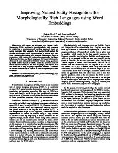
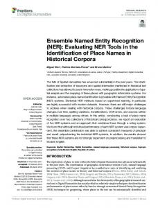
two processes together, therefore we can avoid the error propagation in the pipeline system, and allow the two models to benefit from each other. Part (A) and (B) of Figure 1 show the trellis for decoding word sequence ‘Messi is well-known’ in the NER and NSW detection systems respectively. As shown in (A), every black box with dashed line is a hidden state (possible BIO tag) for the corresponding token. Two sources of information are used in decoding. One is the label transition probability p(yi |yj ), from the trained model, where yi and yj are two BIO tags. The other is p(yi |ti ), where yi is a BIO label for token ti . Similarly, during decoding in NSW detection, we need the

probability of p(oi |oj ) and p(oi |ti ). The only difference is that oi is a NSW label. Part (C) of Figure 1 shows the trellis used in our proposed joint decoding approach for NSW detection and NER. In this figure, three places are worth pointing out: (1) the label is a combination of NSW and NER labels, and thus there are nine in total; (2) the label transition probability is a linear sum of the previous two transition probabilities: p(yi oi |yj oj ) = p(yi |yj ) + β ∗ p(oi |oj ), where yi and yj are BIO tags and oi and oj are NSW tags; (3) similarly, p(yi oi |ti ) equals to p(yi |ti ) + α ∗ p(oi |ti ). Please note all these probabilities are log probabilities and they are trained separately from each system.

4 Basic Features 1. Lexical features (word n-gram): Unigram: Wi (i = 0) Bigram: Wi Wi+1 (i = −2, −1, 0, 1) Trigram: Wi−1 Wi Wi+1 (i = −2, −1, 0, 1) 2. POS features (POS n-gram): Unigram: Pi (i = 0) Bigram: Pi Pi+1 (i = −2, −1, 0, 1) Trigram: Pi−1 Pi Pi+1 (i = −2, −1, 0, 1) 3. Token’s capitalization information: Trigram: Ci−1 Ci Ci+1 (i = 0) (Ci = 1 means this token’s first character is capitalized.) Additional Features by Incorporating Predicted NSW Label 4. Token’s dictionary categorization label: Unigram: Di (i = 0) Bigram: Di Di+1 (i = −2, −1, 0, 1) Trigram: Di−1 Di Di+1 (i = −2, −1, 0, 1) 5. Token’s predicted NSW label: Unigram: Li (i = 0) Bigram: Li Li+1 (i = −2, −1, 0, 1) Trigram: Li−1 Li Li+1 (i = −2, −1, 0, 1) 6. Compound features using lexical and NSW labels: Wi Di , Wi Li , Wi Di Li (i = 0) 7. Compound features using POS and NSW labels: Pi Di , Pi Li , Pi Di Li (i = 0) 8. Compound features using word, POS, and NSW labels: Wi Pi Di Li (i = 0)

Data and Experiment

4.1

Data Set and Experiment Setup

The NSW detection model is trained using the data released by (Li and Liu, 2014). It has 2,577 Twitter messages (selected from the Edinburgh Twitter corpus (Petrovic et al., 2010)), in which there are 2,333 unique pairs of NSW and their standard words. This data is used for training the different normalization models. We labeled this data set using the given dictionary for NSW detection. 4,121 tokens are labeled as ill-OOV, 1,455 as correctOOV, and the rest 33,740 tokens are IV words. We have two test sets for evaluating the NSW detection system. One is from (Han and Baldwin, 2011), which includes 549 tweets. Each tweet contains at least one ill-OOV and the corresponding correct word. We call it Test set 1 in the following. The other is from (Li and Liu, 2015), who further processed the tweets data from (Owoputi et al., 2013). Briefly, Owoputi et al. (2013) released 2,347 tweets with their designed POS tags for social media text, and then Li and Liu (2015) further annotated this data with normalization information for each token. The released data by (Li and Liu, 2015) contains 798 tweets with ill-OOV. We use these 798 tweets as the second data set for NSW detection, and call it Test set 2 in the following. In addition, we use all of these 2,347 tweets to train a POS model which then is used to predict tokens’ POS tags for NER (see Section 3.2 about the POS tags). The CRF model is implemented using the pocket-CRF toolkit5 . The SRILM toolkit (Stolcke, 2002) is used to build the character-level language model (LM) for generating the LM features in NSW detection system.

Table 2: Features used in the NER System. W and P represent word and POS. D and L represent labels classified by the dictionary and 3-way NSW detection system. Subscripts i, i − 1 and i + 1 indicate the word position. For example, when i equals to -1, i + 1 means the current word.

5

933

http://sourceforge.net/projects/pocket-crf-1/

p(IV|IV)

p(B|B)

B

B p(B|Messi)

B

p(IV|Messi)

p(I|B) I

I

p(correct-OOV|Messi) O

O

correct-OOV

correct-OOV

p(ill-OOV|IV)

Ill-OOV

O

IV

p(correct-OOV|IV)

correct-OOV

I

p(O|B)

p(I|Messi)

IV

IV

Ill-OOV

Ill-OOV

is

well-known

p(Ill-OOV|Messi)

p(O|Messi) is

Messi

Messi

well-known

(A)

B_IV

(B) p(B|B)+ β * p(IVIIV)

p(B|Messi)+ α* p(IV|Messi) B_correct-OOV

p(B|B)+ β * p(ill-OOVIIV)

B_IV B_correct-OOV

B_IV B_correct-OOV

p(B|is)+ α* p(correct-OOV|is)

B_ill-OOV

B_ill-OOV p(I|B)+ β * p(IVIIV)

I_IV

I_IV

. . .

. . .

Messi

is

B_ill-OOV p(B|well-known)+ α* p(ill-OOV|well-known) I_IV p(I|B)+ β * p(IVIill-OOV)

. . .

well-known

(C)

Figure 1: Trellis Viterbi decoding for different systems. The data with the NER labels are from (Ritter et al., 2011) who annotated 2,396 tweets (34K tokens) with named entities, but there is no information on the tweets’ ill-OOV words. In order to evaluate the impact of ill-OOV on NER, we ask six annotators to annotate the ill-OOV words and the corresponding standard words in this data. There are only 1,012 sentences with ill-OOV words. We use all the sentences (2,396) for the NER experiments. This data set,6 to our knowledge, is the first one having both ill-OOV and NER annotation in social media domain. For joint decoding, the parameters α and β are empirically set as 0.95 and 0.5. 4.2

in Table 1. First note because of the property of the two-step method (it further divides the OOV words from the dictionary-based method into illOOV and correct-OOV), the upper bound of its recall is the recall of the dictionary based method. We can see that in Test set 1, both the two-step and the 3-way classification methods have a significant improvement compared to the Dictionary method. However, in Test set 2, the two-step method performs much worse than that of the 3-way classification method, although it outperforms the dictionary method. This can be attributed to the characteristics of that data set and also the system’s upper bounded recall. We will provide a more detailed analysis in the following feature analysis part.

Experiment Results

4.2.1

Table 4 and 5 show the performance of the two systems on the two test sets with different features. Note that the dictionary feature is not applicable to the two-step method, and the results for the twostep method using dictionary feature (feature 1, first line in the tables) are the same as the dictionary baseline in Table 3. From these two tables, we can see that: (1) For both systems, normalization features (11∼16) and lexical features (2∼10) both perform better than the dictionary feature. (2) In general, the combination of any two kinds of features has better performance than any one feature type. Using all the features (results shown in Table 3) yields the best performance, which significantly improves the performance compared with the baseline. (3) There are some differences across

NSW Detection Results

For NSW detection, we compared our two proposed systems on the two test sets described above, and also conducted different experiments to investigate the effectiveness of different features. We use the categorization of words by the dictionary as the baseline for this task. Table 3 shows the results for three NSW detection systems. We use Recall, Precision and F value for the ill-OOV class as the evaluation metrics. The Dictionary baseline can only recognize the token as IV and OOV, and thus label all the OOV words as ill-OOV. Both the two-step and the 3-way classification methods in Table 3 leverage all the features described 6

http://www.hlt.utdallas.edu/∼chenli/normalization ner

934

the two data sets in terms of the feature effectiveness on the two methods. On Test set 2, when lexical features are combined with other features (forth and fifth line of Table 5), the 3-way classification method significantly outperforms the twostep method. It is because this data set has a large number of ill-OOV words that are dictionary words. For example, token ‘its’ appears 31 times as ill-OOV, ‘ya’ 13 times, and ‘bro’ 10 times. Such ill-OOV words occur more than two hundred times in total. Since these tokens are included in the dictionary, they are already classified as IV by the dictionary, and their label will not change in the second step. This is also the reason why in Table 3, the performance of 3-way classification is significantly better than that of the two-step method using all the features. However, we also find that when we only use lexical features (2∼10), the two methods have similar performance on Test set 2, but the two-step method has much better performance than the 3-way classifier method on Test set 1. We believe this shows that lexical features themselves are not reliable for the NSW detection task, and other information such as normalization features may be more stable. Test Set 1

System

Features

Two-Step

3-way Classification

R

P

F

R

P

F

1

67.86

69.59

68.72

66.45

64.27

65.34

2∼10

64.33

79.52

71.12

69.56

76.26

72.76

11∼16

53.78

91.34

67.70

54.35

91.42

68.17

1∼10

63.12

81.53

71.16

78.41

81.65

80.00

2∼16

56.40

89.02

69.06

72.32

90.28

80.31

1,11∼16

56.40

92.35

70.03

56.68

92.81

70.38

Table 5: Feature impact on NSW detection on Test Set 2. coding method integrating NER and NSW. This is done using the 1,012 sentences that contain illOOV words. Table 6 shows such results on the NER data described in Section 4.1. The 3-way classification method for NSW detection is used as a baseline here. It is the same model as used in the previous section, and applied to the entire NER data. For each cross validation experiment of the joint decoding method, the NSW detection model is kept the same (from 3-way classification method), but NER model is tested on 1/4 of the data and trained from the remaining 3/4 of the data. From the Table 6, we can see that joint decoding yields some marginal improvement for the NSW detection task.

Test Set 2

R

P

F

R

P

F

Dictionary

88.73

72.35

79.71

67.87

69.59

68.72

System

R

P

Two-step

81.66

88.74

85.05

57.60

90.04

70.26

3-way classification

58.65

72.83

64.97

3-way

87.63

83.49

85.51

73.53

90.42

81.10

Joint decoding w all features

59.53

72.96

65.56

Table 3: NSW detection results. Features

Two-Step

Table 6: NSW detection results on the data from (Ritter et al., 2011) with our new NSW annotation.

3-way Classification

R

P

F

R

P

F

1

88.73

72.35

79.71

87.13

70.04

77.66

2∼10

87.21

77.44

82.04

82.59

67.49

74.28

11∼16

86.45

78.77

82.43

91.75

74.97

82.51

1∼10

76.78

92.87

84.07

77.12

93.09

84.36

2∼16

81.16

89.02

84.90

87.13

86.54

85.30

1,11∼16

78.30

91.00

84.17

78.55

93.77

85.48

F

In the following, we will focus on the impact of NSW detection on NER. Table 7 shows the NER performance from different systems on the data with NER and NSW labels. From this table, we can see that when using our pipeline system, adding NSW label features has a significant improvement compared to the basic features. The F value of 67.4% when using all the features is even higher than the state-of-the-art performance from (Ritter et al., 2011). Please note that Ritter et al. (2011) used much more information than us for this task, such as dictionaries including a set of type lists gathered from Freebase, brown clusters, and outputs of their specifically designed chunk and capitalization labels components7 . Then they

Table 4: Feature impact on NSW detection on Test Set 1. The feature number corresponds to that in Table 1. 4.2.2 NER Results For the NER task, in order to make a fair comparison with (Ritter et al., 2011), we conducted 4-fold cross validation experiments as they did. First we present the result on the NSW detection task on this date set when using our proposed joint de-

7

The chunk and capitalization components are specially created by them for social media domain data. Then they created a data set to train these models.

935

improved their baseline performance from 65% to the reported best one at 67%. However, we only added our predicted NSW labels and related features, and we already achieved similar or slightly better results. Using joint decoding can further boost the performance to 69%. System

R

P

F

Pipeline w basic features

55.85

74.33

63.76

Pipeline w all features

60.00

77.09

67.40

Joint decoding w all features

73.56

65.02

69.00

(Ritter et al., 2011)

73.00

61.00

67.00

tweet ‘Watching the VMA pre-show again ...’, the token VMA is annotated as B-tvshow in NER labels. Without using predicted NSW labels, the baseline system labels this token as O (outside of named entity). However, after using the NSW predicted label correct-OOV and related features, the pipeline NER system predicts its label as B. We noticed that joint decoding can solve some complicated cases that are hard for the pipeline system, especially for some OOVs, or when there are consecutive named entity tokens. For example, in a tweet, ‘Let’s hope the Serie A continues to be on the tv schedule next week’, Seria A is a proper noun (meaning Italian soccer league). The annotation for Seria and A is correct-OOV/B and IV/I. We find the joint decoding system successfully labels A as I after Seria is labeled as B. However, the pipeline system labels A as O even it correctly labels Seria. Take another example, in a tweet ‘I was gonna buy a Zune HD ...’, Zune HD is consecutive named entities. The pipeline system recognized Zune as correct-OOV and HD as ill-OOV, then labeled both them as O. But the joint decoding system identified HD as correct-OOV and labeled ‘Zune HD’ as B and I. These changes may have happened because of adjusting the transition probability and observation probability during Viterbi decoding.

Table 7: NER results from different systems on data from (Ritter et al., 2011). Table 8 shows the impact of different features. This analysis is based on the pipeline system. First, we can see that adding feature 4 and 5 (Uni-, Bi- and Tri-gram of the dictionary and predicted NSW labels) yields the most improvement compared with other features, and between these two kinds of features, using predicted NSW labels is better than the dictionary labels. It also shows the effectiveness of our NSW detection system. Second, comparing adding feature 6 and 7, it shows that combination of word/POS and its dictionary or NSW label is not as good as only considering the label’s n-gram. We also explored various other n-gram features, but did not find any that outperformed feature 4 or 5. Another finding is that the POS related features are not as good as that of words. Features

R

P

F

Basic

55.85

74.33

63.76

Basic + 4

57.71

75.04

65.23

Basic + 5

57.47

75.87

65.37

Basic + 6

56.53

74.20

64.12

Basic + 7

56.13

74.66

64.06

Basic + 8

57.14

74.55

64.66

5

Conclusion and Future Work

In this paper, we proposed an approach to detect NSW. This makes the lexical normalization task as a complete applicable process. The proposed NSW detection system leveraged normalization information of an OOV and other useful lexical information. Our experimental results show both kinds of information can help improve the prediction performance on two different data sets. Furthermore, we applied the predicted labels as additional information for the NER task. In this task, we proposed a novel joint decoding approach to label every token’s NSW and NER label in a tweet at the same time. Again, experimental results demonstrate that the NSW label has a significant impact on NER performance and our proposed method improves performance on both tasks and outperforms the best previous results in NER. In future work, we propose to pursue a number of directions. First, we plan to consider how to conduct NSW detection and normalization at the same time. Second, we like to try a joint method to

Table 8: Pipeline NER performance using different features. The feature number corresponds to that in Table 2. 4.2.3 Error Analysis A detailed error analysis further shows what improvement our proposed method makes and what errors it is still making. For example, for the 936

simultaneously train the NSW detection and NER models, rather than just combining models in decoding. Third, we want to investigate the impact of NSW and normalization on other NLP tasks such as parsing in social media data.

Taku Kudo, Kaoru Yamamoto, and Yuji Matsumoto. 2004. Applying conditional random fields to Japanese morphological analysis. In Proceedings of EMNLP. Vladimir I Levenshtein. 1966. Binary codes capable of correcting deletions, insertions and reversals. In Soviet physics doklady, volume 10, page 707.

Acknowledgments

Chen Li and Yang Liu. 2012a. Improving text normalization using character-blocks based models and system combination. In Proceedings of COLING 2012.

We thank the anonymous reviewers for their detailed and insightful comments on earlier drafts of this paper. The work is partially supported by DARPA Contract No. FA8750-13-2-0041. Any opinions, findings, and conclusions or recommendations expressed are those of the authors and do not necessarily reflect the views of the funding agencies.

Chen Li and Yang Liu. 2012b. Normalization of text messages using character- and phone-based machine translation approaches. In Proceedings of 13th Interspeech. Chen Li and Yang Liu. 2014. Improving text normalization via unsupervised model and discriminative reranking. In Proceedings of ACL.

References

Chen Li and Yang Liu. 2015. Joint POS tagging and text normalization for informal text. In Proceedings of IJCAI.

Aiti Aw, Min Zhang, Juan Xiao, Jian Su, and Jian Su. 2006. A phrase-based statistical model for sms text normalization. In Processing of COLING/ACL.

Fei Liu, Fuliang Weng, and Xiao Jiang. 2012a. A broad-coverage normalization system for social media language. In Proceedings of ACL.

Grzegorz Chrupała. 2014. Normalizing tweets with edit scripts and recurrent neural embeddings. In Proceedings of ACL.

Xiaohua Liu, Ming Zhou, Xiangyang Zhou, Zhongyang Fu, and Furu Wei. 2012b. Joint inference of named entity recognition and normalization for tweets. In Proceedings of ACL.

Paul Cook and Suzanne Stevenson. 2009. An unsupervised model for text message normalization. In Proceedings of NAACL. Fred J Damerau. 1964. A technique for computer detection and correction of spelling errors. Communications of the ACM, 7(3):171–176.

Graham Neubig, Yosuke Nakata, and Shinsuke Mori. 2011. Pointwise prediction for robust, adaptable Japanese morphological analysis. In Proceedings of ACL.

Kevin Gimpel, Nathan Schneider, Brendan O’Connor, Dipanjan Das, Daniel Mills, Jacob Eisenstein, Michael Heilman, Dani Yogatama, Jeffrey Flanigan, and Noah A. Smith. 2011. Part-of-speech tagging for twitter: Annotation, features, and experiments. In Proceedings of ACL.

Olutobi Owoputi, Brendan O’Connor, Chris Dyer, Kevin Gimpel, Nathan Schneider, and Noah A. Smith. 2013. Improved part-of-speech tagging for online conversational text with word clusters. In Proceedings of NAACL. Deana Pennell and Yang Liu. 2010. Normalization of text messages for text-to-speech. In ICASSP.

Bo Han and Timothy Baldwin. 2011. Lexical normalisation of short text messages: Makn sens a #twitter. In Proceeding of ACL.

Deana Pennell and Yang Liu. 2011. A character-level machine translation approach for normalization of sms abbreviations. In Proceedings of IJCNLP.

Hany Hassan and Arul Menezes. 2013. Social text normalization using contextual graph random walks. In Proceedings of ACL.

Sasa Petrovic, Miles Osborne, and Victor Lavrenko. 2010. The Edinburgh twitter corpus. In Proceedings of NAACL.

Nobuhiro Kaji and Masaru Kitsuregawa. 2014. Accurate word segmentation and pos tagging for Japanese microblogs: Corpus annotation and joint modeling with lexical normalization. In Proceedings of EMNLP.

Vivek Kumar Rangarajan Sridhar, John Chen, Srinivas Bangalore, and Ron Shacham. 2014. A framework for translating SMS messages. In Proceedings of COLING.

Dilek Kucuk and Ralf Steinberger. 2014. Experiments to improve named entity recognition on turkish tweets. In Proceedings of Workshop on Language Analysis for Social Media (LASM) on EACL.

Alan Ritter, Sam Clark, and Oren Etzioni. 2011. Named entity recognition in tweets: an experimental study. In Proceedings of EMNLP.

937

Cagil Sonmez and Arzucan Ozgur. 2014. A graphbased approach for contextual text normalization. In Proceedings of EMNLP. Andreas Stolcke. 2002. SRILM-an extensible language modeling toolkit. In Proceedings International Conference on Spoken Language Processing. Aobo Wang and Min-Yen Kan. 2013. Mining informal language from Chinese microtext: Joint word recognition and segmentation. In Proceedings of ACL. Yi Yang and Jacob Eisenstein. 2013. A log-linear model for unsupervised text normalization. In Proceedings of EMNLP.

938