Improving Phase Estimation with Enhanced Turbo Decoders Bartosz Mielczarek, Arne Svensson Communication Systems Group Department of Signals and Systems Chalmers University of Technology SE-412 96 Göteborg, Sweden PH: +46 31 772 1763 FAX: +46 31 772 1748, e-mail:
[email protected],
[email protected] ABSTRACT This paper discusses a realistic turbo coding system when the signal phase has not been perfectly estimated. We propose improved decoding algorithms for the situations when the residual phase error can be modelled by the Gaussian probability distribution and a Markov chain, a model which can be used in many actual phase estimators. It is shown that increasing the state space of the decoders can dramatically improve the bit error probability without the need of increasing transmitted power. INTRODUCTION On of the most important factors determining the efficiency of a wireless system is the power required for successful transmission of data. The required power needed to reliably transmit a signal can be reduced by using special coding techniques. One of the latest and the most prominent of such techniques is turbo coding with a performance which is almost able to reach the Shannon channel capacity limit [1]. The problem lies, however, in the practical applications of the turbo codes. Unfortunately, reducing the transmitted power makes it more difficult to estimate the channel and properly synchronize the phase of the incoming signal. In our paper we propose algorithms aiming at improving performance of turbo-coded systems with non-perfect phase offset estimation.
x ks
uk
Interleaver
RSC Enc. 1
x kp, 1
RSC Enc. 2
x kp, 2
Figure 1: Turbo encoder architecture not work without a proper phase estimation and must rely on some initial estimates of the signal phase. If, on the other hand, the phase estimator/decoder knows the structure of the data signal, it can use this knowledge in joint phase and data estimation and improve the system’s performance. We will use this approach for the algorithms presented in this paper. TURBO ENCODER A typical turbo encoder ([1],[2]) of rate 1/3 is shown in figure 1. It consists of two recursive, systematic, convolutional encoders RSC1 and RSC2, separated by a pseudorandom interleaver. The incoming sequence of data u k generates the systematic bits x ks = u k and the parity bits x kp, 1 , x kp, 2 created by the encoders RSC1 and RSC2, respectively. The stream of code bits is BPSK-modulated and transmitted over an AWGN channel as real-valued signal samples c k using the BPSK modulation format [5]. THE SYSTEM MODEL
PHASE SYNCHRONIZATION Good phase synchronization is essential in all digital wireless communication. The incoming HF signal needs to be downconverted to lower frequency ([3],[4]) which requires exact knowledge of carrier frequency and phase. There exists a number of different techniques to estimate the carrier parameters (such as Phase Locked Loops, Costas loops and averaging filters) but none of these algorithms succeed to provide perfect estimation of the carrier signal. One of the reasons for such performance loss is that synchronization of phase is done before the decoding process. This is due to the fact that most decoders will
The system analysed in this paper is presented in figure 2. The encoded signal suffers from a phase noise process θ k which can be a result of a fading process or oscillator instability. After that, the signal is corrupted by the white, Gaussian noise. The incoming distorted signal is fed to the phase synchronizer, which produces estimates of the phase noise process θˆ k . After adjusting the phase error, the signal is decoded (the decoded data sequence can then be used to refine the phase estimation process). Formally, the signal after the AWGN channel, phase estimation and receiver matched filtering (the timing recovery is assumed to be perfect) can be expressed as
e data bits
j θk
n k = N ( 0, N 0 )
Turbo encoder
Turbo decoder e –jθk
decoded bits
ˆ
- rate 1/3 - (031,037) component codes - 1000 bit interleaver
Remaining phase error: φ k = θˆ k – θ k = N ( 0, σ φ2 )
Phase estimator
Figure 2: System model yk = e
j φk
(1)
ck + n k
where y k is the complex received signal (which can be the systematic bit y ks , the first parity bit y kp, 1 or the second parity bit y kp, 2 ) and n k is the white, additive, Gaussian complex noise with E [ n k 2 ] = N 0 . φ k is the phase offset estimation error θˆ k – θ k and its statistics are discussed in the next section. GENERAL PHASE ERROR MODELLING The phase error φ k can be modelled as Gaussian distributed, with known variance σ φ2 and zero mean for non-biased phase estimators (which are the most common solutions [3]). Such an assumption is rather popular in the existing literature and seems to be quite realistic, since typical synchronizers produce an error distribution with a similar shape and known variance (for example, the Tikhonov distribution after the PLL loop, see [5]). Moreover, since the phase estimation is usually an effect of some kind of averaging of the initial signal, the phase error values will be correlated. A new approach to this problem is modelling the actual sign of the phase error (which tends to remain constant for a number of samples) as a simple Markov chain. This way we introduce a simple memory model to the channel which is relatively easy to incorporate into the turbo decoder. By using the above unified framework (graphically shown in figure 3) to model the phase error, our approach can be tailored to many existing phase synchronizers, just by applying the actual phase error variance and the crossover probability for the phase error sign change in the Markov model. Even though more complicated models can be used, our approach achieves quite good results without increasing the decoding complexity too much. Phase error distribution
Phase error sign model 1-p p
φ0 1-p
Figure 3: Phase error modelling
p
TURBO DECODING ALGORITHM Due to the presence of the interleaver in the decoder, the optimal decoding of turbo codes would be very complex. The practical sub-optimal implementations split the process into two separate processes, in which both component codes are decoded independently [2]. The connection between the codes is implemented by exchanging soft extrinsic information and using a form of the MAP decoding (minimizing the probability of the bit error) for each component code. The most commonly used decoding algorithm is the BCJR-MAP algorithm ([6]) which computes the soft bits using the log likelihood ratio (LLR) (see [2]) P ( u k = +1 Y ) L ( u k Y ) = log --------------------------------- P ( u k = -1 Y )
(2)
where Y is the whole received code sequence. The LLR is calculated as α˜ ˜ k ( s ) k – 1 ( s′ ) ⋅ γ k ( s′ ,s ) ⋅ β S+ L ( u k Y ) = log ----------------------------------------------------------------------- (3) α˜ ˜ ( s ) k – 1 ( s′ ) ⋅ γ k ( s′ ,s ) ⋅ β k S
∑ ∑
where α˜ k ( s′ ) and β˜ k ( s ) are the recursively calculated probabilities of arriving at state s′ (computed from the start of the trellis) and state s (computed form the end of the trellis), respectively (for details see [2]). The term γ k ( s′ ,s ) is the apriori probability of the transition between states s′ and s and is given by γk ( s′ ,s ) = p ( u k )p ( y k u k ) 1 1 ∝ exp --- u k ( L e ( u k ) + Lc y ks ) exp --- L c y kp x kp 2 2
(4)
where L e ( u k ) and L c = 4E c /N 0 are the extrinsic information about bit k (calculated by the first decoder, e ( u ) , or by the second decoder, L e ( u ) ) and the L 12 k 21 k channel reliability factor of the decoder ( E c is the code bit energy), respectively. The numerator of the MAP equation (3) includes all the transitions which correspond to data bit u k = +1 ( S + ) and the denominator all the transitions which correspond to u k = – 1 ( S - ).
Uncorrected signal φ
Deinterleaver
Perfect BPSK signals Received signals Corrected signals
e (u ˆ k) L 21
e (φ ˆ k) L21
APP Dec. 1 Wrong rotation
y kp, 1
y kp, 2
APP Dec. 2
e (φ ˆ k) L 12
Correct rotation Interleaver
e (u ˆ k) L 12
y ks
Interleaver
Figure 5: Modified decoder architecture with additional soft phase information exchange
Figure 4: Phase error reduction principle LARGE PHASE ERROR CORRECTION The loss in performance is caused mainly by large phase errors which result from long tails of the error distribution. Luckily, the large phase errors are easier to detect than small ones, which suggests that the synchronization algorithm can concentrate primarily on reducing them instead of trying to correct all phase errors [7]. Correcting phase errors is equal to rotating the received signal samples in the opposite direction of the actual phase error. The two parameters which must be known prior to such correction are the size and the sign of the actual phase offset. Assuming that we know the size of the rotation (discussed later) the remaining uncertainty is the sign of the offset. One of the ways to detect it is to create two sets of samples y k ( + ) and y k ( - ) as yk ( ± ) = y k e±j φ
(5)
where φ is the rotation size, and use the decoder to compare their metrics. Figure 4 shows the principle of the algorithm operation. An initial phase error rotates the received BPSK signal points away from the correct positions. By rotating the received signal in two opposite directions we create one signal which lies closer to the optimum position than the other, facilitating detection since the distance between signal alternatives increases.
The proposed decoder architecture is shown in figure 5. Two specially modified APP decoders are connected in a feedback loop, exchanging soft data information and soft phase error sign information (discussed later in the paper) for all symbols. The two streams of soft messages are properly interconnected using interleavers and deinterleavers (compare with encoder shown in figure 1). The modification to the APP decoders will be explained in next sections. MODIFIED TRANSITION PROBABILITY In order to incorporate the phase rotation algorithm, the transition probability from equation (4) is redefined as γ k ( s′ ,s φ ks , φ kp ) = p ( u k )p ( y k u k, φ ks , φ kp )p ( φ ks , φ kp ) 1 ∝ p ( φ ks, φ kp ) exp --- u k L e ( u k ) 2
(7)
1 1 ⋅ exp --- L c y kp ( φ kp ) x kp exp --- u k L c y ks ( φ ks ) 2 2 where the received samples y ks and y kp are conditioned on the offset sign events φ ks and φ kp , respectively, having the joint probability distribution p ( φ ks, φ kp ) . Such a modification suggests that additional states and transitions are needed in the decoder to detect the sign of the offsets. GENERAL MODIFIED APP DECODER
GENERAL DECODER MODIFICATION To detect the sign of the phase offset, equation (2) can be reformulated in the following form P ( φ k > 0 Y ) (6) L ( φ k Y ) = log ----------------------------- P ( φ k < 0 Y ) which is the LLR of the probability that the k-th code bit had the positive phase error and the probability of the negative phase error. One of the ways to solve equation (6) is to use the turbo technique, i.e., use two decoders to iteratively improve estimation of the rotation signs.
In general the phase error sign can vary from one signal sample to the other. Even if it can be modelled as the Markov chain, the use of channel interleaver (a widely used solution aiming at combating the burst errors, common in wireless channel.) may effectively remove the correlation between consecutive phase error signs. To fully represent such a situation, we have to split each original state (due to the code) into four different states, one representing two positive shifts denoted henceforth as (+,+), one representing two negative transitions (,-) and two with mixed error signs (+,-) and (-,+).
the systematic phase offsets are common for both component codes), are given as
Rotations of the received bits:
S (+,+)
(ej φ , ej φ
S (+,-)
)
( e j φ , e –j φ )
S ( -, + )
( e –j φ , e j φ
S (-,-)
Figure 6: General modification of the trellis transition Figure 6 shows the construction of the trellis for one bit transition. The probability of the transitions are defined as p k(+,+) = p ( φ ks > 0, φ kp > 0 )
p k(-,+ )
=
p ( φ ks
< 0,
φ kp
(10)
p k(-,+) = p k(-,-) = 1 – p k(+,+)
(11)
)
( e –j φ , e –j φ )
p k(+,-) = p ( φ ks > 0, φ kp < 0 )
e, s ( φ ) ) exp ( L 21 k p k(+,+) = p k(+,-) = -------------------------------------------e, s ( φ ) ) 1 + exp ( L 21 k
(8)
> 0)
p k(-,-) = p ( φ ks < 0, φ kp < 0 ) These probabilities can be initially set to values reflecting the a-priori information (when the Markov model is used) or be set equal (if no initial phase correlation is expected). The enhanced APP decoder works in a usual way using the BCJR algorithm except that four times as many states have to be included in equation (3). Moreover, the transition probabilities are calculated using equations (7) and (8). In this way, the extrinsic information about phase offsets can be calculated after a decoding pass, hopefully with the majority of the rotations correctly detected. After the decoding pass, the decoder produces soft information about the information bits and, in addition to that, phase information about systematic bits as α˜ k – 1 ( s′ ) ⋅ γ k ( s′ ,s ) ⋅ β˜ k ( s ) (+,*) e, s ( φ ) = log S-----------------------------------------------------------------------L 12 - k . α˜ k – 1 ( s′ ) ⋅ γ k ( s′ ,s ) ⋅ β˜ k ( s ) S (-,*)
∑ ∑
where S (+,*) are the S (+,+) and S (+,-) states and S (-,*) are the S (-,+) and S (-,-) states. The soft phase information about the parity bits is produced as α˜ k – 1 ( s′ ) ⋅ γ k ( s′ ,s ) ⋅ β˜ k ( s ) (*,+) e, p ( φ ) = log S-----------------------------------------------------------------------L 12 - (9) k α˜ k – 1 ( s′ ) ⋅ γ k ( s′ ,s ) ⋅ β˜ k ( s ) S (*,-)
these probabilities are then passed to the second decoder (after proper interleaving) along with the soft information bits and the same procedure is repeated. SIMPLIFIED FIRST APP DECODER If no channel interleaver is used, there is a large probability that both systematic and parity bits, (fed directly to the first APP decoder, see figure 5) will experience phase errors with the same signs. This fact can be used to simplify the construction of the first APP decoder and improve the performance of the system (the second decoder cannot be simplified, due to the interleaving of the systematic bits). The structure of the simplified trellis is shown in figure 7. As it can easily be seen, the number of states is doubled and the number of transition calculation is increased four times compared to the original unmodified trellis. With the above assumption the probability distribution p ( φ ks , φ kp ) reduces to a one dimension distribution, with the values defined as p k(+,+) = p ( φ ks > 0, φ kp > 0 )
The probabilities of these transitions are initially set to reflect the Markov chain parameters (see figure 7) and are progressively modified when the soft bit messages are passed between the decoders as explained in the previous section.
where S (*,+) are the S (+,+) and S (-,+) states and S (*,-) are the S (+,-) and S (-,-) states. The transformations between the actual probabilities and soft information can be derived from equation (6) and, assuming that the phase offsets are independent (i.e., only
p k(+,+)
S (+,+) S (-,-)
S (+,+) S (-, -)
p k(-,-) p k(+,+)
Rotations of the received bits: ej φ
∑ ∑
(12)
p k(-,-) = p ( φ ks < 0, φ kp < 0 )
e –j φ
S (+,+) p k(-,-)
S (-,-)
Initial transition weights p
S (+,+) S ( -, -)
1–p
S (+,+) 1–p
p
S (-,-)
Figure 7: First modified APP decoder and the initial weights for transitions
The soft value of the phase error information is calculated as α˜ k – 1 ( s′ ) ⋅ γ k ( s′ ,s ) ⋅ β˜ k ( s ) (+,+) e ( φ ) = log S------------------------------------------------------------------------L 12 (13) k ˜α k – 1 ( s′ ) ⋅ γ ( s′ ,s ) ⋅ β˜ ( s ) k k S (-,-)
∑ ∑
where the numerator of the MAP equation includes all the transitions caused by double positive rotation states ( S (+,+) ) and the denominator the transitions caused by double negative rotation states ( S ( -,-) ). The assumption of the correlated phase error signs can be extended to the second parity bit as well, which will slightly change the exchange of the phase information between the APP decoders. Since, after the first APP decoding, the soft phase error sign information has to be interleaved for the systematic bits, the transformation between the actual probabilities and soft information passed to the second decoder will be given as e ( φ )) e (φ )) exp ( L 12 exp ( L 12 l k p k(+,+) = ------------------------------------------ ------------------------------------------e ( φ ) ) 1 + exp ( L e ( φ ) ) 1 + exp ( L 12 l 12 k
(14)
e (φ )) exp ( L 12 1 k p k(+,-) = ------------------------------------------- ------------------------------------------e ( φ ) ) 1 + exp ( L e ( φ ) ) 1 + exp ( L 12 k 12 k
(15)
p k(-,-) = 1 – p k(+,+)
p k(-,+) = 1 – p k(+,-)
(16)
e ( φ ) is the soft phase value corresponding to where L 12 l the systematic signal before interleaving as e ( φ ) = Π ( L e ( φ )) L 12 k 12 l
(17)
where Π is the interleaver function. Also the feedback phase information message from the second APP decoder to the first APP decoder has to be modified. This is done by combining the information about the systematic and parity offsets ([9]) to obtain the e ( φ ) as final soft phase value L 21 k
ALGORITHM PERFORMANCE To test the performance gains and discuss the properties of the algorithm we chose to employ a system experiencing a very strong phase noise. The synchronizer uses a residual carrier which is Wiener-filtered to track the rapid changes of the phase. Such systems have been proposed for deep-space communications [8] and their properties are similar to the very fast fading wireless channels. The phase noise process is generated by a program reflecting actual phase noise characteristics of a deep-space communication link (oscillator instability). The parameter p of the Markov channel is empirically calculated to be around 0.6. The rotation of the samples was chosen to be the expected value of the absolute value of the phase error as ∞
φ =
∫
φ p φ ( φ ) dφ
(21)
–∞
Note, that such a rotation provides optimal performance in terms of resulting phase error variance only if all the phase error sign decisions were perfect. The discussion of the rotation optimization will be presented in a separate paper. The simulations were conducted with the CCSDS (023,033) turbo code ([10]) and an interleaver size of N=1000. The number of decoding iterations was set to 10. All BER calculations were done using data from 10000 transmitted blocks with independent, randomly generated parameters. Figure 8 presents the behaviour of the proposed phase offset algorithm for different phase error variances. It improves the BER performance of the traditional scheme, introducing a gain of approximately 0.1-0.2dB. The gain is particularly visible for low quality phase estimation and in the region of large SNRs. 0
10
-1
10
Perfect synchronization Unmodified decoder Modified decoder
L e, s ( φ ) + L e, p ( φ )
k 21 1 + e 21 l e ( φ ) = log ------------------------------------------------(18) L 21 k e , p e , s L (φ ) L (φ ) e 21 l + e 21 k e, p ( φ ) is the soft phase value corresponding to where L21 l the parity signal before deinterleaving as
e, p ( φ ) L 21 k
=
e, p ( φ ) ) Π – 1 ( L 21 l
φ
σ2=0.3
-3
φ
10
σ2=0.2
-4
(19)
where Π – 1 is the inverse interleaver function. Finally, the transition probabilities are calculated as e (φ )) exp ( L21 k p k(+,+) = ------------------------------------------- , p k(-,-) = 1 – p k(+,+) e (φ )) 1 + exp ( L 21 k
σ2=0.4
-2
10
φ
10
σ2=0.1
-5
φ
10
-6
10
(20)
0
0.5
1
1.5
2
2.5
Eb/N0 [dB]
Figure 8: BER performance of the improved decoder (circled line), classical decoder (crossed line) and the system with ideal synchronization (solid line) for different phase error variances.
Initially, the simulations of the system showed that repeated exchange of the soft phase information leads to convergence to the incorrect solution. The reason for it is that the correlation between the samples (high crossover probability) is rather small and the successive iterations do not contribute a lot of new information to the soft phase information. After noticing this, the algorithm was slightly modified by turning of the feedback from the second APP decoder to the first APP decode, which eliminated the convergence problem. Moreover, increasing number of iterations proved to further improve the performance of the enhanced system. Unfortunately, due to the time and computer capacity constraints, these results could not be presented here and will be discussed in future papers.
ACKNOWLEDGEMENTS This work was supported by the Swedish Foundation for Strategic Research under the Personal Computing and Communication grant, a scholarship of Telefonaktiebolaget LM Ericsson’s Stiftelsen för främjande av elektroteknisk forskning and a scholarship of Stiftelsen för internationalisering av högre utbildning och forskning (STINT). REFERENCES [1]
[2] CONCLUSIONS Phase synchronization is currently one of the biggest problems when implementing turbo codes in real wireless systems. In this paper we introduced a general method of modelling the phase estimation errors, which can be used with different phase synchronizers. This method was then used to modify the classical turbo decoder structure and proved to improve the performance, even in a very severely distorted system. The analysis of the proposed solution is still incomplete and further research is still necessary. It is not quite clear how the iterative process will proceed with different types of phase errors, preliminary results suggest that the soft phase information exchange must be terminated when the correlation between phase samples is low. Moreover, the discussion of the specific system parameters such as the rotation value must follow. It turns out, for example, that there is a optimal rotation value, unique for every set of phase error parameters. It is, however, relatively safe to say that a lot is to be gained by incorporating phase synchronization into the turbo decoder. Such solutions may be the only way to combat heavily distorted channels expected when the carrier frequency increases.
[3] [4]
[5] [6]
[7]
[8]
[9]
[10]
Berrou, C., Glavieux, A., Thitimajshima, P., “Near Shannon limit error-correcting coding and decoding: turbo codes,” ICC 1993, pp. 1064-1070. Barbulescu, S.A., Iterative Decoding of Turbo Codes and Other Concatenated Codes, PhD Dissertation, University of South Australia, 1996. Meyr, H., Moeneclaey, M., Fechtel, S.A., Digital Communication Receivers, Wiley 1998 Mengali, U., D’Andrea, A.N., Synchronization Techniques for Digital Receivers, Plenum Press 1997 Proakis, J.G., Digital Communications, McGrawHill 1995 L. Bahl, J. Cocke, F. Jelinek, and J.Raviv, “Optimal decoding of linear codes for minimizing symbol error rate,” IEEE Trans. Inf. Theory, pp. 284287, Mar. 1974 B. Mielczarek, Synchronization in Turbo Coded Systems, Licentiate thesis, Department of Signals and Systems, Chalmers University of Technology, Göteborg, Sweden, 2000 D. Divsalar, J.Hamkins, B.Mielczarek, “Coupled receiver-decoders,” Proceedings IEEE Information Theory Symposium, Washington, D.C., USA, June 2001, submitted. J. Hagenauer, “The Turbo Principle: Tutorial and State of the Art,” Proceedings International Symposium on Turbo Codes and Related Topics, Brest, France, pp. 1-11, Sept. 1997 Consultative Committee for Space Data Systems, 101.0-B-4: Telemetry Channel Coding, Blue Book. May 1999