Improving resource use efficiency in rice-based cropping systems ...

Improving resource use efficiency in rice-based cropping systems: Experimentation and modelling

Promotor: Prof.dr.ir. H. van Keulen Hoogleraar bij de Leerstoelgroep Plantaardige Productiesystemen, Wageningen Universiteit

Co-promotoren: Dr.ir. H. Hengsdijk Plant Research International, Wageningen Universiteit en Researchcentrum Dr.ir. B.A.M. Bouman International Rice Research Institute (IRRI), Philippines

Promotiecommissie: Prof.dr.ir. Huub Spiertz Wageningen Universiteit Prof. Wang Guanghuo Zhejiang University, Hangzhou, China Dr. Michael Dingkuhn Centre de Coopération Internationale en Recherche Agronomique pour le Développement (CIRAD), Montpellier, France Dr.ir. Hein ten Berge Plant Research International, Wageningen Universiteit en Researchcentrum

Dit onderzoek is uitgevoerd binnen de 'C.T. de Wit'-onderzoekschool: Production Ecology and Resource Conservation.

Improving resource use efficiency in rice-based cropping systems: Experimentation and modelling

Qi Jing

Proefschrift ter verkrijging van de graad van doctor op gezag van de rector magnificus van Wageningen Universiteit Prof.dr. M.J. Kropff in het openbaar te verdedigen op vrijdag 9 november 2007 des ochtends te elf uur in de Aula.

Qi Jing, 2007 Improving resource use efficiency in rice-based cropping systems: Experimentation and modelling Ph.D. Thesis, Wageningen University, Wageningen, the Netherlands, —with ref.— - with summaries in English and Dutch ISBN: 978-90-8504-774-2

Abstract Jing, Q., 2007. Improving resource use efficiency in rice-based cropping systems: Experimentation and modelling. PhD thesis, Wageningen University, Wageningen, the Netherlands. With summaries in English and Dutch, 145 pp.

To cope with the projected increase in food demand and increased environmental concerns, rice-based cropping systems combining high resource use efficiencies and high yields will be increasingly important. By combining experimental research with crop growth simulation, this study aims at a better quantitative understanding of crop production and nitrogen dynamics in irrigated rice-wheat (RW) systems to improve N management as a basis for the design of RW systems that combine high yields with high N use efficiencies. The various field experiments included different rice genotypes, environments, and N fertilizer and water management. Experimental data was used to evaluate the rice crop growth model ORYZA2000, which performed satisfactorily. The model was applied to explore options for different N management regimes combining high yields and high nitrogen use efficiency, and to identify the relative importance of environmental factors affecting yield and nitrogen use efficiency. Average rice yields of around 10-11,000 kg ha-1 were simulated with fertilizer N rates of around 200 kg ha-1, with high nitrogen use efficiency in three equal splits at transplanting, panicle initiation and booting at Nanjing, China. Indigenous soil N supply affects yield and internal N use efficiency (INUE, kg grain per kg N uptake) more than weather at low N rate, but its effect is reduced at high N rate. Temperature contributes more than radiation to the variation in rice yield, N uptake and INUE. The study resulted in better understanding of the relationship between yield and N dynamics in rice-based systems and in a RW model integrating existing crop and soil models and using results from own experiments. This model is a promising research tool to design and to develop rice-based cropping systems with high yields and high resource use efficiencies. Key words:

Nitrogen; Yield; Rice; Wheat; Environment; Simulation; Soil; Organic matter; Water; Denitrification

Acknowledgements I like to express my sincere gratitude to many people, both from my professional and personal life, for their contribution to the realization of this thesis. I would like to thank Weixing Cao for introducing me to the project ‘Water-less rice’ that supported my sandwich PhD fellowship at the C.T. de Wit Graduate School for Production Ecology and Resource Conservation (PE&RC) of Wageningen University. Thank you for your help during my professional career and your care and attention for my personal life. From the start of my career, I appreciate your steady support and suggestions for improving my work. Before I came to Wageningen, I was told to be lucky to have Herman van Keulen as my supervisor. When I met him for the first time in Beijing, I immediately felt his warmth and friendliness, giving me confidence that I was on the right track. I benefited much from his experience and knowledge during my study. Many thanks Herman, your patience, direct comments, and detailed editing enabled me to complete this thesis. I met Huib Hengsdijk in China in 2002 and later he became my cosupervisor. I am indebted to you, Huib, I can not describe how much I learned from you during our numerous discussions. Your supervision took me through many difficult stages from writing the proposal till the completion of my thesis. I enjoyed working with you and I am grateful for your support in my personal life and for facilitating my stay in Wageningen. I like to thank Bas Bouman for his efficient supervision at the International Rice Research Institute (IRRI). Thank you Bas; I had an exciting time with you when you introduced me in the field of modelling and model evaluation. Our collaboration was rewarded with the publication of a peer-reviewed paper in an international journal, which would not have been possible without your inspiration and support. I would like to extend my thanks to Prem Bindraban for his attention for my personal life and my thesis work. Thank you Prem, I am grateful for your hospitality and the discussions at your home. I appreciate your relentless support, for example, when I passed an important and difficult exam. The celebration of this joyful event organized by you - helped me to pass other courses. I thank Ken Giller for his comments during the PPS lunch meetings and for the dinner at his place. I also like to thank Huub Spiertz for his comments on my thesis, and for the sight-seeing trip in the Netherlands. Peter Leffelaar gave helpful suggestions on N modelling in the early stages of my study. Gon van Laar provided model software and gave useful advice on using the models. I benefited from the discussions with Xinyou Yin during proposal writing. Raymond Jongschaap helped me to improve my programming skills and provided the model and software on which Chapter 6 is based. Sjaak Conijn and

Jacques Withagen provided me with tips and tricks in program checking and statistics, respectively. I thank Irene Gosselink, Elise ter Horst-Jacobs, Mira Teofanović and Ria van Dijk for facilitating my work at Wageningen UR. I sincerely thank Peter Uithol for his help during my stay at PRI, especially in editing the thesis while I was in China. I will never forget my friends in Wageningen, with whom I chatted and who helped me: Putu, Impron, Christina, Vaia, Ken, Iwan, Jiayou, Xiaozhun, Jane, Else, Senthi, Jouke, Miyuki, Zhongshan, Miqia, Caiyun, Xuekui, Lijin, Yehong, Jianjun, Wen Jiang, Lizhen, Shipeng, Jun Liu, Meixing, Lingzhi, Huaidong, Nan Luo, Shujun, Fuyu, Jianwei, Jihua, Hanping, Wenfeng, Guiwen, Lu Zhang, Xingfeng and Tang. I have had a great time at IRRI and I benefited from many friends, especially Liping Feng. Thank you Liping, for your help in model calibration and validation. I enjoyed our trips in the Philippines. I like to thank Shaobing Peng for his kind words when I was at IRRI, and his advice on data analysis. I was happy to meet Alice, Annie and Dule at IRRI, and to meet them later in Wageningen again. I will not forget the dinners with you in Los Baños, nor the drinking and chatting in Wageningen. I thank all my friends for sharing beers, discussions, the hot spring, sports and dinners at IRRI: Xiaoguang Yang, Yuhua Shan, Haiming Li, Jianlong Xu, Hehe, Kaifeng, Juan Liu, Huanzhe, Jianmin, Lixiao, Jianfu, Junxing and Bing. Great thanks go to my colleagues in China, especially to Tingbo Dai and Dong Jiang, thank you guys. I learned much from you, and I appreciate your support during my PhD study, wherever I was, in Nanjing or abroad. I sincerely acknowledge many people participating in the ARICENET project ‘Development of a Rice Simulator Interfacing Gene Function to Field Performance’, Particularly the support of Mrs. Sasaki, Tamura and Akita (Iwate Agricultural Experimental Center), Mr. Kuroda (Iwate University), Mrs. N. Inoue and Hagiwara (Shinshu Univiversity), Mrs. Kobata, Ohnishi and Kobayashi (Shimane University), Mrs. T. Horie, T. Shiraiwa, Nakagawa, Matsui and K. Katsura (Kyoto University), Mr. Jongkaewwattana (ChiangMai University), Mr. W. Zou (Yunnan Agricultural University) and Mrs. X. Liu and X. Wang (Nanjing Agricultural University). Their dedicated work contributed much to Chapter 2 and 3 of this book. I greatly thank my parents and parents-in-law, my sister and brother for looking after my family when I was absent. My daughter HuanHuan has encouraged me (unknowingly) to finish my thesis rapidly when she called me ‘Pa Pa’ over the phone. She still recognized my voice after such a long period of separation; it really excited me and provided the final push to finish the thesis. Special thanks are for my wife Yunzhi Zhu. Thank you Yunzhi, for your understanding and for taking care of our

HuanHuan during my absence. I could not have completed this study without your support. Finally, I thank all of you whom I have not mentioned by name, but I remember our meetings, joint experiences and whatever we shared, I give my best wishes to you and your families.

Funding This publication is sponsored by the Partners in Water for Food program. The Government of the Netherlands initiated the Partners in Water for Food program in the backdrop of the Second World Water Forum, held in 2000 in The Hague. At that meeting seven challenges were identified, founded on the overriding and generally accepted concept of Integrated Water Resources Management. “Partners in Water for Food” is focused on the challenge of securing the world's food supply, particularly of the poor and vulnerable, in a situation of increasing demands for water. It responds to this challenge through a program of capacity building, knowledge exchange and cooperation between partners in different countries. In line with Integrated Water Resources Management, the program emphasizes the need for comprehensive solutions in managing water demand for the production of food. The program operates under the theme 'Capacity Building for Agricultural Water Demand Management'.

Table of Contents

1 General introduction ................................................................................................ 1 1.1 Background........................................................................................................ 1 1.2 Challenges in rice-based cropping systems ....................................................... 3 1.3 Simulation of rice-based cropping systems ....................................................... 4 1.4 Objectives .......................................................................................................... 5 1.5 Outline of the thesis ........................................................................................... 5 2 The performance of five rice genotypes in tropical and subtropical environments: Grain yield and quality .................................................................. 7 Abstract....................................................................................................................... 7 2.1 Introduction........................................................................................................ 8 2.2 Materials and methods..................................................................................... 10 2.3 Results.............................................................................................................. 13 2.4 Discussion........................................................................................................ 22 2.5 Conclusions...................................................................................................... 25 3 Analysis of environmental factors affecting yield and N uptake of irrigated rice in Asia using a modelling approach .............................................. 27 Abstract..................................................................................................................... 27 3.1 Introduction...................................................................................................... 28 3.2 Materials and methods..................................................................................... 29 3.3 Results.............................................................................................................. 34 3.4 Discussion........................................................................................................ 43 3.5 Conclusions...................................................................................................... 46 4 Exploring options to combine high yields with high nitrogen use efficiencies in irrigated rice in China ....................................................................................... 47 Abstract..................................................................................................................... 47 4.1 Introduction...................................................................................................... 48 4.2 Material and methods ...................................................................................... 49 4.3 Results.............................................................................................................. 54 4.4 Discussion and conclusions ............................................................................. 66 5 Quantifying N response and N use efficiency in Rice-Wheat (RW) cropping systems under different water management ........................................................ 69 Abstract..................................................................................................................... 69 5.1 Introduction...................................................................................................... 70

5.2 5.3 5.4 5.5

Material and methods ...................................................................................... 71 Measurements .................................................................................................. 72 Results.............................................................................................................. 74 Discussion and conclusions ............................................................................. 81

6 Modelling nitrogen and water dynamics in rice-wheat rotations ...................... 85 Abstract..................................................................................................................... 85 6.1 Introduction...................................................................................................... 85 6.2 Model description ............................................................................................ 87 6.3 Model evaluation ............................................................................................. 96 6.4 Discussion and conclusions ........................................................................... 101 7. General discussion ................................................................................................ 105 7.1 Options to increase yield and quality............................................................. 106 7.2 Options to increase resource use efficiency................................................... 108 7.3 Approaches of modelling and experimentation............................................. 111 7.4 Concluding remarks....................................................................................... 112 References.................................................................................................................. 115 Summary.................................................................................................................... 129 Samenvatting ............................................................................................................. 133 PE&RC PhD Education Certificate........................................................................ 137 Curriculum vitae....................................................................................................... 139 Selected peer-reviewed publications during Ph.D. study...................................... 141

1

General introduction

1.1

Background

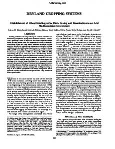
In next two decades world food demand is projected to increase with 60% due to the growing population (Cassman, 1999; FAO, 2003; Khush, 2005). Especially in Asia, population growth rates are high, while the demand is further increased through the shift in Asian diets from staples towards livestock and dairy products associated with the fast growing economies (Pingali, 2007). Rice is the major staple crop in Asia, from the cool sub-tropics to the warm humid tropics (Fig. 1.1). The total rice area in Asia is about 143 Mha, of which 73 Mha are irrigated, producing more than 70% of the global rice production (IRRI, 2002). In the tropics, two- or three-seasons of rice production per year are possible, depending on the availability of water. Only one rice crop per year can be grown in part of the sub-tropics, due to low temperatures in the winter period. Instead, winter crops, such as wheat and rapeseed, are grown in rotation with rice. Of these, rice-wheat (RW) cropping systems occupy 26 Mha in Asia, mainly in the Indo-Gangetic Plains (IGP) and the Yangtse River Basin of China (Fig. 1.2). Main characteristic of these RW-systems is the alternation of anaerobic (flooded) and aerobic soil conditions under rice and wheat, respectively (Timsina and Connor, 2001). China’s rice area currently totals about 30 Mha, of which 90% is irrigated (Huang et al., 2001), and 9-13 Mha is rotated with winter wheat, according to different estimates (Dawe et al., 2004; Huke et al., 1993; Ladha et al., 2003; Timsina and Connor, 2001). The potential to expand the area for cereal production is limited because suitable land is scarce (Tong et al., 2003). The current agricultural area is even expected to decrease in the future due to the increasing competition for land by urbanization and industrial development (Brockherhoff, 2000; Chen, 2007). Therefore, increased production per unit of area needs to be the main strategy to produce more food for a growing population. Rice yields strongly vary over Asia, from less than 2 Mg ha-1 to more than 15 Mg ha-1 (Horie et al., 1997; Romyen et al., 1998; Whitbread et al., 2003; Ying et al., 1998a, b), depending on location and variety. A major cause of yield differences is the variation in environmental conditions, i.e. climate and soil (Horie et al., 1997; Ying et al., 1998a). In general terms, yield is the result of the interaction of Genotype (cultivar characteristics), Environment (climate and soil conditions) and Management (irrigation and fertilizer regime). The relative importance of each of these factors on yield in various environments is still poorly understood.

2

IMPROVING RESOURCE EFFICIENCY IN RICE-BASED CROPPING SYSTEMS

Figure 1.1

Agroecological zonation of Asia. Dominant agroecological zones: 1. warm semi-arid tropics; 2. warm sub-humid tropics; 3. warm humid tropics; 5. warm semi-arid sub-tropics with summer rainfall; 6. warm sub-humid subtropics with summer rainfall; 7. warm/cool humid sub-tropics with summer rainfall; 8. cool sub-tropics with summer rainfall. (Source: IRRI, 2002).

Figure 1.2

Distribution of RW production areas in South Asia and China. The curve passing from northeast to southwest China represents the limits for growing RW sequences in China (Source: Timsina and Connor, 2001).

1 GENERAL INTRODUCTION

1.2

3

Challenges in rice-based cropping systems

Especially the use of mineral fertilizers in China has contributed to the spectacular yield increase in RW systems between the 1960's and 1990's. Recent studies show that yields of both crops stabilize and do not increase as rapidly as in the past (Fig. 1.3). As a result, agronomic efficiency of nitrogen, i.e. the incremental increase in grain yield that results from N application, deceased in rice from 160 kg kg-1 in 1961 to 10 kg kg-1 in 1996, and in wheat from 44 to 6 kg kg-1 (Tong et al., 2003). Among the provinces with intensive RW cropping systems in China, average fertilizer N input is highest in Jiangsu with rates of about 500 kg N per ha per year (Zhu et al., 2000). Associated fertilizer N recovery is 30~35% in both crops (Li et al., 2000; Peng et al., 2002; Zhu and Chen, 2002). On the one hand, excessive N fertilizer rates have increased emissions of greenhouse gases and pollution of water resources (Richter and Roelcke, 2000; Xing and Zhu, 2000; Zhang et al., 1996; Zhu et al., 2000; Zhu et al., 2003; Zhu and Chen, 2002), while on the other hand increased fertilizer inputs have increased production costs resulting in lower net returns for farmers (Wang et al., 2001). Future rice-based crop production should aim at high yields combined with high nitrogen use efficiency, thus increasing farmers’ profitability and limiting negative environmental externalities.

8000

Yield kg ha

-1

6000 5000

300

4000 200

-1

400

N application kg ha

7000

500 Rice yield Wheat yield N input

3000 2000 1985

Figure 1.3

1990

1995

2000

100 2005

Year Trends in N input and yields of rice and wheat in RW systems in China. Yields and N inputs are the means of Jiangsu, Anhui, Hubei and Sichuan Provinces. Bars are the deviations of N inputs among provinces (Source: China Statistical Yearbook, 2004).

4


Irrigated rice-based cropping systems are among the major water users in Asia and account for around half of all diverted freshwater in Asia. Rice is usually irrigated with 2 to 3 times more water than other irrigated cereals (Tuong et al., 2005). The increasing scarcity of water and competing claims on water by other sectors (CA, 2007; FAO, 2003) require that agriculture uses water resources more efficiently than in the past. Recent research has focused on water-saving technologies, especially in rice cultivation. A range of new irrigation and cultivation methods have been developed, which basically consist of growing rice under more aerobic conditions, i.e. no continuous flooding during the growing season. Avoidance of a continuous water layer reduces water losses due to percolation, drainage and evaporation (Bouman et al., 2007). The alternation of aerobic and anaerobic field conditions in rice systems affects the sustainability of rice production, environmental impact, and N dynamics.

1.3

Simulation of rice-based cropping systems

Cropping systems consist of numerous complex and interacting biological processes, which can be influenced by human management. Quantification of these complex processes helps to increase understanding of crop growth and facilitates the design of new management strategies aimed at combining high yields and high resource use efficiencies. Modelling is an important tool to explicitly describe the relationships between the various components of complex systems (Jones et al., 2003; Keating et al., 2003; Van Ittersum et al., 2003). It increases insight into relevant processes, allows study of the effects of crop management, and exploration of possible consequences of management modifications. Once a model has been parameterized and validated, it can be used in support of analysis and interpretation of field experiments, for extrapolation of experimental results over a wider range of management practices and weather conditions, and to explore and derive, for example, efficient N management strategies (Bouman et al., 1996). Since the 1980’s, many crop models have been developed (Hoogenboom et al., 2004; Jones et al., 2003; Keating et al., 2003; Van Ittersum et al., 2003). The crop growth models CERES-Rice and CERES-Wheat (CERES, Crop Estimation through Resource and Environment Synthesis) have been applied for studying RW systems in northern Bangladesh and northwest India (Sarkar and Kar, 2006; Timsina et al., 1998). Existing models have problems simulating RW systems as various soil processes perform quite differently under anaerobic and aerobic conditions, a main feature of these systems (Probert, 2002; Shibu et al., 2006; Timsina and Connor, 2001; Timsina

1 GENERAL INTRODUCTION

5

and Humphreys, 2006). A comprehensive modelling framework that is able to simulate crop growth under both contrasting soil conditions does not yet exist.

1.4

Objectives

This study aims at better understanding of crop growth and nitrogen dynamics in irrigated RW systems as a basis for improved N management in these systems as a component in the design of RW systems that combine high yields of the desired quality with high N use efficiency. I combine experimental and modelling approaches to improve insight in the underlying processes.

•

•

• •

Specific objectives of my study comprise: Quantification of the contribution of genotype and environment to yield and grain quality, and identification of the relative importance of environmental factors affecting yield and N use efficiency of rice. Assessment of the relative effects of indigenous soil N supply and N-fertilizer regimes on yield of irrigated rice, as a basis for the design of improved N management strategies for high-yielding and N use efficient irrigated rice-wheat systems in China. Analysis of the N response and N use efficiency in RW systems through a dedicated field experiment. Development of a rice-wheat rotation model (RIWER) for quantification of N dynamics and exploration of management options aimed at high resources use efficiency in RW systems.

1.5

Outline of the thesis

The background and justification of this study are described in this Chapter. Based on results of a multi-location rice experiment across Asia, Chapter 2 quantifies the effects of genotype, environment and their interactions on grain yield and quality. Data from these experiments in combination with the rice growth model ORYZA2000 are used in Chapter 3 to analyse the contribution of environmental factors to yield and N use efficiency. Chapter 4 examines N management strategies to increase N use efficiency in rice using a modelling approach. Chapter 5 describes the results of a two-year RW experiment aimed at quantifying N response and N use efficiency in RW systems. A RW-simulation modelling framework has been developed, based on existing models

6


and aiming at comprehensive analysis of RW systems. The model RIWER (RIce WhEat Rotation) is described in Chapter 6. Finally, general conclusions are presented and prospects for model application in resource use analysis and management are discussed in Chapter 7.

2

The performance of five rice genotypes in tropical and subtropical environments: Grain yield and quality

Qi Jing1,2,3, Huib Hengsdijk2, Herman van Keulen2,3, Weixing Cao1, Tingbo Dai1 1

2

3

Hi-Tech Key Lab of Information Agriculture of Jiangsu Province, Nanjing Agricultural University, Nanjing 210095, China Plant Research International, Wageningen University and Research Centre, P.O. Box 16, 6700 AA Wageningen, the Netherlands Plant Production Systems Group, Wageningen University, P.O. Box 430, 6700 AK Wageningen, the Netherlands

Abstract The consequence of the still rapidly growing population of Asia is an increasing demand for rice with well-defined grain quality characteristics. Yield and quality of rice depend on the interaction between genotypic characteristics and environmental conditions. This study describes the results of field experiments in eight agroecological zones of the tropics and subtropics across Asia during 2001 and 2002. The aim of the standardized experiments was to study the performance of five rice genotypes in terms of yield, harvest index (HI) and quality (protein and amylose content) in different environmental conditions. The genotypes included Japonica× indica crossbred Takanari, indica IR72, japonicas Nipponbare and Takenari, and the indica×javanica crossbred IR65564-44-2-2. There were significant differences in grain yield, HI, protein content, and amylose content among genotypes. Averaged over locations and years, yields and HIs of Takanari were highest, while amylose content of IR72 was highest. Environmental differences explained 80% of the observed variation in grain yields, and 66% of the variation in HIs. Low yields at tropical locations were associated with low radiation interception, resulting from fast phenological development during the vegetative phase, and low HI resulting from poor grain formation during the reproductive phase. The variation among genotypes in yield and HI could be well described by second order polynomial equations based on average temperature during the ripening period (ATR). Amylose content of rice grains differed among genotypes, which explained 72% of the total variation, compared to 24% by environmental conditions. Grain amylose content was linearly and inversely correlated to ATR. Protein content was not

8


significantly different among locations mainly because of the similar N management across experiments. Results may support selection of genotypes for targeted yield and quality characteristics under well-defined environmental conditions, and provides information for adapting crop management (e.g. sowing date). In addition, the multi-location data set can be used to improve dynamic rice simulation models with respect to simulation of grain quality and better characterization of different rice genotypes. Key words: yield formation; harvest index; protein content; amylose content.

2.1

Introduction

Asia's irrigated rice area of 73 Mha produces more than 70% of the global rice production (Maclean et al., 2002). About two-thirds of this area is located in the tropics and the remainder in the subtropics (Hossain and Laborte, 1993). To cope with the projected population growth and the associated increase in food demand, average irrigated rice yields in Asia must increase with 60% from 4.9 t ha-1 to 8 t ha-1 in 2025 (IRRI, 1995). Yields in tropical areas are often below 5 t ha-1 (Dobermann et al., 2003a; Romyen et al., 1998; Whitbread et al., 2003), while those in subtropical areas often exceed 6 t ha-1 (Dobermann et al., 2003a; Horie et al., 2003; Jing et al., 2005). Past research has compared the productivity of rice in subtropical and tropical areas to identify growth factors contributing to this difference. For example, Ying et al. (1998a) found in two years that the same high-yielding genotypes yielded 33 and 62% more under subtropical than under tropical conditions. In these experiments, under optimum management and ample supply of water and nutrients, temperature and radiation were the main yield-determining factors (Van Ittersum and Rabbinge, 1997). However, effects of these climatic factors were not further analyzed in these experiments. Horie et al. (1997) reported that irrigated rice yields were affected by genotypic characteristics, location and their interaction (G×E). However, they did not quantify the contribution of the individual factors to the yield variance. Remarkably, very few attempts have been made to analyze the performance of irrigated rice across subtropical and tropical areas in Asia. Where available, such reports are descriptive and do not explain yield differences (Ying et al., 1998a). Sound comparison among sites is only possible when experiments are carried out and data collected according to standard protocols. This is difficult to realize, which may explain the scarcity of systematically collected empirical information on the

2 THE PERFORMANCE OF FIVE RICE GENOTYPES . . .

9

interaction between rice genotypes and environments across Asia. Better understanding of genotype-environment interactions facilitates design of new genotypes, identification of test conditions, and genotype selection for specific welldefined conditions (Jackson et al., 1996; Yan and Hunt, 1998). Yield is a function of biomass production and the proportion of that biomass invested in the grains (harvest index, HI) (Cock and Yoshida, 1972; Murata and Matsushima, 1975). Future yield increase must result from improvements in one or both components (Farrell et al., 1998). Intercepted photosynthetically active radiation (IPAR) and crop-specific radiation-use efficiency (RUE, biomass produced per unit of IPAR) determine biomass production. Assimilates for grain filling originate from photosynthesis after flowering and from reserves stored in culms and leaves during the vegetative period. Longer crop growth durations, leading to higher radiation interception, result in higher yields if associated with favorable RUE and HI. High temperatures during vegetative growth stages accelerate crop development, shortening crop growth duration, resulting in lower grain yields. The photothermal quotient (PTQ, the ratio of average radiation intensity to average temperature during the grain filling period) has been proposed as a single indicator to capture the combined effect of the yield-determining factors radiation and temperature on yields (Nix, 1976). As basic food security in Asia improves, demand for rice with superior quality properties increases. Grain quality will become even more important in the future, when the economic situation of the very poor—many of whom depend on rice as their staple food—improves and they demand higher quality rice (Juliano and Villareal, 1993). The nutritional value of rice is related to its protein content, while its amylose content is an important indicator of cooking and consumption quality (Juliano, 1985; Lii et al., 1996). Low amylose content increases water absorption, volume expansion, and stickiness of cooked rice (Delwiche et al., 1996), while high amylose content is associated with hard grains after cooking (Juliano, 1998). Preferences for soft and hard rice grains vary widely across Asia. Quality characteristics of rice are formed during grain filling, and are determined by environmental and genotypic factors and their interactions. However, these interactions are poorly understood, which hampers breeding of rice varieties with targeted quality characteristics. Systematic data on quality characteristics of different rice varieties grown under tropical and sub-tropical conditions are scarce. The objective of this study is to compare and evaluate grain yield and grain quality (protein content and amylose content) among five rice genotypes (G) in two tropical and six subtropical environments (E) in Asia, and to examine their variation on the basis of environment × genotype interactions (G×E). To realize this objective, multi-location experiments with these genotypes have been carried out, using a


10

standard protocol, which are described in the section materials and methods. In the results section, variations in grain yield and quality among genotypes and locations and their interactions are analyzed. To better understand and explain the results, RUEs, PTQs and the relationships between on the one hand average temperature during ripening (ATR) and on the other hand yield, HI and grain amylose content are quantified. Finally, results are discussed with respect to their contribution to the rice research agenda.

2.2

Materials and methods

2.2.1

Experimental locations

The two-year multi-varietal field experiments were carried out in South and East Asia in the framework of the Asian Rice Network (ARICENET) (Horie et al., 2003), according to a standard protocol for experimental design, crop management, observations, measurements and processing of collected data. In 2001, there were seven experimental sites of which five in subtropical regions, i.e. Iwate, Nagano, Kyoto and Shimane in Japan, and Nanjing in China, and two in tropical regions, i.e. Chiangmai and Ubon in Thailand (Fig. 2.1). In 2002, the subtropical location Taoyuan in China was added.

JAPAN CHINA

THAILAND

Figure 2.1

Site Latitude Iwate 39o32’ Nagano 35o52’ Kyoto 35o03’ Shimane 35o27’ Nanjing 32o20’ Taoyuan 25o59’ Chiangmai 18o48’ Ubon 15o20’

Agroecological zone Cool subtropics Cool subtropics Cool subtropics Cool subtropics Warm subhumid subtropics Warm/cool humid subtropics Warm subhumid tropics Warm subhumid tropics

Location of the experimental sites and the agroecological zonation based on Maclean et al. (2002).


2.2.2

11

Experimental design and crop management

At each experimental site, five genotypes were tested, including indica, japonica, indica×japonica, and indica×javanica types (Table 2.1). All experiments had a randomized block design with 3 replicates and a plot size of 20 m2. At transplanting, 40 kg N ha-1 was applied, and 20 kg N ha-1 was top-dressed every 20 days until 10 days after heading, so that N fertilizer supply (in kg ha-1 d-1) varied from 0.94 at Nagano and Shimane to 1.05 at Chiangmai. In addition, 120 kg P2O5 ha-1 and 120 kg K2O ha-1 were applied as a basal dressing. Rice seedlings with 4 to 5 leaves, depending on genotype, were transplanted at 2 plants hill-1, spaced at 30 cm between the rows and 15 cm within. During the experiments, experimental fields were continuously flooded, and weeds, pests and diseases were adequately controlled by biocides. Table 2.1 Genotypes, their acronyms, plant type and characteristics. Genotype Acronym Plant type Characteristic Takanari TA indica×japonica crossbred High-yielding IR72 IR indica IRRI standard IR65564-44-2-2 NP indica×javanica crossbred New plant type of IRRI Nipponbare NI japonica Japanese standard Takenari TE japonica Japan old genotype

2.2.3

Observations and measurements

The vegetative period is defined in this study as time from emergence to panicle initiation, the reproductive period from panicle initiation to flowering, and the ripening period from flowering to maturity. Panicle initiation was identified as the moment that the panicle was visible as a white feathery cone of 1.0-1.5 mm in the main culm, flowering as the moment the stamen were visible, while maturity was recorded when less than 10-15% of the grains was still green-colored. At transplanting, 20 plants were sampled for each genotype; at 20 days after transplanting, panicle initiation, two weeks before flowering, flowering, two weeks after flowering, and at maturity, eight hills per genotype were harvested for green leaf area measurement, and leaf area index (LAI) was calculated. At maturity, plants were partitioned into leaves, stems combined with sheathes, and panicles, and were dried till constant weight in an oven at 80 ºC. Spikelet numbers per panicle were measured, the spikelet fertility was determined from the number of filled grains per panicle, filled grains were selected in a NaCl solution with a specific gravity of 1.03. Grain yield were measured on a plot of 2 m2, yield was

12


expressed at a moisture content of 14%. Harvest index (HI) was defined as grain yield divided by total aboveground dry weight. Protein and amylose contents of rice grains were determined in Iwate, Kyoto and Nanjing in 2001, and in Shimane, Nanjing, Taoyuan and Chiangmai in 2002. Grain samples were threshed milled and ground in preparation for protein and amylose analysis. N content was determined by micro-Kjeldahl digestion, distillation, and titration, and converted to protein content by multiplication by 5.95 (Juliano and Villareal, 1993). Amylose content was determined according to the modified assay described by Juliano et al. (1981) and Juliano and Villareal (1993). Daily weather data recorded at weather stations at each experimental location, included radiation (RD) and maximum (Tmax) and minimum (Tmin) temperature.

2.2.4

Data analysis

GenStat for Windows, 8th Edition (http://www.vsn-intl.com/genstat/) was used in data analysis, i.e. establishing effects of genotype, location and year, and their interactions on yield, harvest index, protein content and amylose content. The method of residual maximum likelihood (REML) was used, which provides efficient estimates of treatment effects in unbalanced designs and allows analysis of incomplete data sets (data of Taoyuan for 2001 were missing) (Welham and Thompson, 1997). Statistical differences were determined using Wald statistics. Average values of analyzed variables for the two years are given when the year × genotype interaction was not significant. GenStat was also used to determine regressions of daily average temperature during ripening (ATR) on yield, HI, and amylose content. Intercepted photosynthetically active radiation (IPAR) was calculated from radiation: IPAR = 0.5 × RD × (1 − e − k×L )

(eqn 2.1)

where k is the light extinction coefficient of rice, which is set to 0.4-0.6 depending on the crop development stage as used in the rice crop growth model ORYZA2000 (Bouman et al., 2001); L is daily leaf area index of the canopy, calculated by linear interpolation from measured LAI at various growth stages. PTQ is defined by Nix (1976) as the ratio of mean daily total incident solar radiation for an interval to the mean temperature minus a base temperature. It is a gross measure of light energy available for photosynthesis per unit of developmental


13

unit, a high PTQ indicates that more biomass is produced per developmental unit. Considering the differences in crop phenology at the different locations, PTQ was calculated over a period of 30 days prior to anthesis (Islam and Morison, 1992), using intercepted radiation (Fischer, 1985): PTQ =

IRD 0.5 × (Tmin + Tmax ) − Tb

(eqn 2.2)

where IRD is intercepted radiation, calculated from measured radiation using equation (1), Tmin and Tmax are daily minimum and maximum temperature, respectively, while Tb is the base temperature, for rice set to 8 °C.

2.3

Results

2.3.1

Weather and growth duration

Daily average radiation and temperature during the three phenological stages at the eight locations are shown in Table 2.2. The variation in radiation among growth periods was in general smaller in both tropical locations than in the sub-tropical areas. On average, radiation was higher in the subtropical locations during the vegetative and reproductive growth periods, but was highest in both tropical locations, Chiangmai and Ubon, during the ripening period. Table 2.2

Daily average incoming radiation and average temperature during the vegetative (V), reproductive (Re), and ripening (Ri) stages of rice at eight locations in Asia (average of 2001 and 2002). Daily average radiation ± sd (MJ m-2 d-1) Daily average temperature ± sd (oC) Location V sd Re sd Ri sd V sd Re sd Ri sd Iwate 15.7 0.04 13.3 0.27 10.6 0.49 18.9 0.22 23.1 0.05 16.6 0.91 Nagano 19.1 0.18 20.2 0.89 13.9 0.50 20.2 0.24 24.2 0.26 22.1 0.69 Kyoto 15.5 0.13 15.1 0.24 12.5 0.24 22.9 0.26 27.7 1.05 25.0 0.57 Shimane 16.0 0.11 18.7 0.51 13.0 0.70 21.1 0.28 27.8 0.33 23.6 0.87 Nanjing 15.4 0.02 14.4 0.31 14.1 0.22 27.2 0.06 27.7 0.66 24.8 0.78 Taoyuan 18.6 0.11 16.8 1.49 15.3 1.62 25.2 0.11 25.6 0.63 24.2 0.35 Chiangmai 14.9 0.55 16.0 0.24 15.9 0.21 28.1 0.16 27.7 0.37 26.2 1.11 Ubon 17.0 0.18 16.1 0.74 15.8 0.71 28.5 0.06 28.2 0.15 27.7 0.22 Vegetative is from emergence to panicle initiation, reproductive from panicle initiation to flowering, ripening from flowering to maturity. sd is standard deviation for the five genotypes.


14

Daily average temperature in subtropical locations was highest during the reproductive growth period, while in tropical locations it was lower during the ripening period than during the vegetative period. Average daily temperature during ripening was lowest in Iwate (16.6 oC), i.e. about ten degrees lower than in Chiangmai and Ubon. The large standard deviation of daily temperature during ripening at Chiangmai is associated with large differences in growth duration of genotypes at this location. Average lengths of the phenological stages, i.e. vegetative, reproductive, and ripening, at each location are shown in Fig. 2.2. At the subtropical locations, the vegetative and ripening periods were longer, while the reproductive periods were shorter than at the tropical locations. At the subtropical locations, the vegetative periods were substantially longer than the reproductive and ripening periods, while in both tropical locations, the vegetative periods were much shorter, at Ubon even shorter than the reproductive period. Ripening periods at Chiangmai and Ubon were on average shorter than those at the subtropical sites. Days 110 100 90 80 70 60 50 40 30 20 Iwate

Shinshu

Kyoto

Shimane

Nanjing

Taoyuan Chiangmai

Ubon

Sites

Vegetative

Figure 2.2

Reproductive

Ripening

Average length of the three phenological stages of five rice genotypes at eight experimental sites in Asia. Vegetative phase is from emergence to panicle initiation, reproductive from panicle initiation to flowering, ripening from flowering to maturity. Bars in each column represent the standard deviation among five genotypes.


2.3.2

15

Yield

Yield variation across locations and genotypes Average yields across experimental locations were significantly different among the five genotypes (Table 2.3). In general, yields of the indica×japonica crossbred (TA) and the indica genotype (IR) were higher than those of the japonica genotypes (NI and TE) and the indica×javanica crossbred (NP). TA attained the highest average yields and the new genotype developed at IRRI (NP) the lowest. Table 2.3

Genotype TAa IR NP NI TE

Average grain yield, harvest index (HI), protein content and amylose content of five rice genotypes across different locations in South and East Asia in two years (2001 and 2002). Yield (kg ha-1) Harvest index(-) Protein content (%) Amylose content (%) 7613 ab 0.48 A 8.0 a 8.5 d 6619 b 0.42 B 7.1 ab 19.9 a 5430 c 0.35 C 7.0 b 10.3 bc 5880 c 0.41 B 7.4 ab 9.7 c 5932 c 0.39 Bc 7.5 ab 10.8 b

Source of variation and its contributionc Location (L) 0.807 (**) 0.655 (**) (NS) 0.238 (**) Genotype (G) 0.092 (**) 0.215 (**) 0.266 (*) 0.721 (**) L×G 0.101 (**) (NS) (NS) 0.041 (**) Year (*) (*) (*) (**) Year × G (NS) (NS) (NS) (NS) a See Table 2.1 for explanation of acronyms. b Within a column, values followed by different letters (a-d) are significantly different at the 0.05 probability level. c Calculated as sum of square (SS) of environment divided by total SS (SST). *, ** Significant at the 0.05 and 0.01 probability levels.

Grain yields were consistently low at Iwate, Chiangmai and, especially, Ubon (Table 2.4). Yields for all five genotypes were highest in Taoyuan, while Kyoto scored second for TA, IR, NP, and TE in both years. Location explained 80.7% of the yield variation (sum of squares), genotype 9.2%, and the remainder was due to their interaction (Table 2.3).


16

Grain yields (kg ha-1) of five genotypes at different locations in Asia (average of 2001 and 2002). Genotype Location a TA IR NP NI TE Average b Iwate 6593 c 3902 de 2957 e 5360 c 5308 c 4824 Nagano 9093 b 6164 c 5850 bcd 7679 ab 7558 b 7269 Kyoto 10009 ab 9145 a 7159 ab 6769 bc 6758 bc 7968 Shimane 9097 b 8580 ab 6868 bc 7257 b 7134 b 7787 Nanjing 8527 b 6906 bc 5310 cd 6500 bc 6878 bc 6824 Taoyuan 10928 a 10618 a 9301 a 9749 a 10432 a 9920 Chiangmai 4564 d 5456 cd 5029 d 1939 d 1978 d 3793 Ubon 1646 e 2184 e 966 f 1448 d 1499 d 1505 a See Table 1 for explanation of acronyms; b Within a column, values followed by different letters (a-f) are significantly different at the 0.05 probability level.. Table 2.4

Response to temperature during ripening The relationship between average daily temperature during the ripening phase (ATR) and yield (Y) can be described by a polynomial (Fig. 2.3): Y = Ymax + s( x − ATRmax ) 2

(eqn 2.3)

where Ymax is maximum yield under given crop management, ATRmax optimum ATR for obtaining Ymax and s a shape parameter describing the steepness of the curves. The parameter s (Table 2.5) is constant for all genotypes (s = -172.5), indicating constant relative decline in yields per degree temperature difference from optimum ATR. ATRmax of the indica and indica-japonica crossbred genotypes, TA and IR, is significantly higher than that of the japonica genotypes, indicating the better adaptation of the latter to lower temperatures during ripening. At optimum ATR, Ymax of NP under the management applied, is lower than those of the other genotypes, that do not show significant differences, in contrast to the yields obtained in the experiments (Table 2.4). This implies that for these genotypes ATR was suboptimal in the experiments.


17

-1

Yield (kg ha ) 12000 10000

TA IR

8000

NI

NP

TA

NI

6000

TE

TE

NP

15

20

IR

4000 2000 0 10

25

30 o

Daily average temperature during ripening ( C)

Figure 2.3

Relation between yield and average daily temperature during the ripening stage for the different genotypes at different sites in Asia during 2001 and 2002. See Table 2.1 for explanation of acronyms of genotypes.

Table 2.5

Parameters of fitted curves of second order polynomials for yield (Ymax) and harvest index (HI) on daily average temperature during the ripening phase. Genotype Yield HI b Ymax se ATRmax se s se HImax se ATRmax se s se a TA 9579 585 22.1 0.45 -172.5 18.7 0.56 0.03 22.3 0.53 -0.006 0.0008 IR 8711 566 22.0 0.39 id. id. 0.50 0.02 22.2 0.46 id. Id. NP 7579 556 21.5 0.38 id. id. 0.43 0.02 21.7 0.45 id. Id. NI 9441 682 21.1 0.38 id. id. 0.53 0.03 21.8 0.45 id. Id. TE 9368 657 20.6 0.38 id. id. 0.50 0.03 21.3 0.44 id. Id. a See Table 2.1 for explanation of acronyms b se is standard error.

PTQ analysis Yield for all genotypes was positively and significantly correlated with the PTQ 30 days prior to anthesis (Fig. 2.4), although the relation was different for the japonica genotypes, TE and NI, on one hand and the indica IR and the crossbreds TA and NP on the other hand. In general, the japonica genotypes show higher yields at lower PTQs and lower yields at higher PTQs than the indica and the crossbreds, suggesting lower yield increase per unit of developmental time for the japonica genotypes.


18

-2

Yield (g m ) 1200

Y1 = 1771.6x - 748.12

TA IR NP NI TE

1000 800 600

2

R = 0.673**

Y2 = 752.21x + 20.564 2

R = 0.8389** 400 200 0 0

0.2

0.4

0.6

0.8 -2

-1 o

Photothermal quotient (MJ m d

Figure 2.4

2.3.3

1

1.2

-1

C )

Relation between grain yield and photothermal quotient 30 days prior to anthesis in two years for different genotypes at different locations in Asia. Solid line (Y1) is for indica IR and crossbreds TA and NP; dotted line (Y2) is for japonica cultivars. ** Correlation coefficients significant at 0.01 level. See Table 2.1 for explanation of acronyms.

Radiation use efficiency (RUE)

Radiation use efficiency varied among genotypes between 1.87 and 2.11 g MJ-1, as illustrated in Fig. 2.5 for specific locations. RUE also varied among locations for the same genotype. Maximum RUE was around 2.8 g MJ-1 at Taoyuan, followed by 2.3 g MJ-1 at Chiangmai, while at Nagano, Kyoto, Shimane and Nanjing RUEs ranged from 1.8 to 2.0 g MJ-1. Average RUEs at Iwate and Ubon were 1.6 and 1.5 g MJ-1, respectively.


19

-2

Total aboveground biomass (g m ) 2500

6

2000

TA

66

6 6 3 4 3 4 3 424 31 443113 1 1 2 44 42 53 7 1 12 3 47 3 2 7 5 535 5 5 5 11 75 1 75

IR NP

1500

NI TE 1000 78 500

e1=2.8 e2=1.7

0 0

77 8

77

8 88 8

8

8

200

400

600

800

1000

-2

Intercepted PAR (MJ m )

Figure 2.5

2.3.4

Relation between total aboveground biomass (dry matter) and total intercepted photosynthetically active radiation (PAR). Numbers near the symbols refer to the locations: 1 Iwate; 2 Shinshu; 3 Kyoto; 4 Shimane; 5 Nanjing; 6 Taoyuan; 7 Chiangmai; 8 Ubon. See Table 2.1 for explanation of acronyms. e1 is the slope of the solid line, e2 is the slope of the dotted line.

Harvest index (HI)

Variation across locations and genotypes The high yield of TA was associated with a HI significantly higher than those of the other genotypes (Table 2.3), whereas NP had the lowest HI. Overall, high yields in the experiments were associated with high HIs. Average HI for a specific genotype varied significantly among experimental locations (Table 2.6), from the lowest in Ubon, via Iwate, Chiangmai, Taoyuan, Shimane, Kyoto and Shinshu, to the highest in Nanjing, illustrating the effect of environmental conditions on HI. HI was thus lowest for the most northern and most southern location, i.e. Iwate (39° N) and Ubon (15° N). Differences in environmental conditions among the locations explain 65.5% of the variation in HI, genotypes 21.5% (Table 2.3).


20

Table 2.6

Harvest index (HI) of five genotypes at different locations in Asia (average of 2001 and 2002). Genotype Location a TA IR NP NI TE Average b Iwate 0.42 bc 0.27 b 0.20 b 0.33 b 0.30 b 0.31 Nagano 0.55 ab 0.45 a 0.38 a 0.49 a 0.49 a 0.47 0.50 a 0.46 a 0.41 ab 0.40 ab 0.46 Kyoto 0.56 ab Shimane 0.52 ab 0.48 a 0.41 a 0.42 ab 0.41 ab 0.45 0.51 a 0.42 a 0.53 a 0.45 ab 0.50 Nanjing 0.60 a Taoyuan 0.50 ab 0.48 a 0.42 a 0.42 ab 0.36 ab 0.44 0.38 ab 0.35 a 0.34 b 0.34 b 0.37 Chiangmai 0.44 b Ubon 0.28 c 0.28 b 0.15 b 0.35 ab 0.35 ab 0.28 a See Table 1 for explanation of acronyms b Within a column, values followed by different letters (a-e) are significantly different at 0.05 probability level.

Response to temperature We used a similar polynomial equation as in Section 2.3.2 to describe the relation between HI and ATR (Table 2.5). Parameter s is constant for all genotypes (s = -0.006), indicating constant relative decline in HI per degree temperature difference from optimum ATR. ATRmax for the indica genotype IR and the indica-japonica crossbred TA is higher than that for the japonica genotype TE, i.e. maximum HI of the japonica is attained at lower ATR. The model suggests that HI under optimum ATR could have been about 0.1 higher than in the experiments (Table 2.3).

2.3.5

Protein content

Average protein content varied from 7.0 to 8.5% (Table 2.3), with the highest value for the indica-japonica crossbred TA and the lowest for the indica-javanica crossbred NP. Protein contents were not significantly different among locations, suggesting that environmental factors, e.g. temperature and radiation, hardly affected protein content.

2.3.6

Amylose content

Average amylose content varied from 8.5 to 19.9% and differed significantly among genotypes (Table 2.3), with the highest value for IR and the lowest for TA. Amylose content was similar in both years for all genotypes, but significantly different among


21

locations, i.e. highest in Iwate and lowest in Chiangmai (Table 2.7), indicating effects of environmental factors. Amylose content increased linearly and significantly with decreasing ATR (Fig. 2.6) for both japonica genotypes and both crossbreds, for IR the the trend was similar but non-significant. Table 2.7

Grain amylose content (%) of five genotypes at different locations in Asia (average of 2001 and 2002). Genotype Location a TA IR NP NI TE Average b Iwate 12.7 a 21.6 a 15.0 a 15.4 a 15.4 a 16.3 Kyoto 7.7 bc 17.8 c 9.3 bc 9.3 b 10.5 bc 11.1 Shimane 8.7 bc 20.8 ab 9.9 b 10.7 b 10.7 bc 12.1 Nanjing 7.5 c 20.7 ab 9.7 b 7.4 c 10.0 c 11.1 Taoyuan 9.7 b 19.6 bc 10.3 b 9.3 b 11.65 b 12.1 Chiangmai 4.6 d 19.0 c 7.9 c 5.2 d 6.6 d 8.7 a See Table 2.1 for explanation of acronyms. b Within a column, values followed by different letters (a-d) are significantly different at the 0.05 probability level.

Amylose content (%)

y = -0.2574x + 25.79

25

2

R = 0.382 20 TA

15

NP NI

10

5

TE

y = -0.7373x + 26.965

IR

R = 0.8559**

2

0 10

15

20

25

30 o

Daily average temperature during ripening ( C)

Figure 2.6

Relation between daily average temperature during the ripening phase and amylose content for different genotypes at different locations in Asia. See Table 2.1 for explanation of acronyms. ** Correlation coefficients significant at 0.01 level.

22


2.4

Discussion

2.4.1

Grain yield

About 80% of the observed variation in yield is explained by differences in environmental factors (E), while genotype (G) and interactions (G×E) each contribute 10%. These proportions could change for other combinations of genotypes and environments, but environmental factors contribute most to yield variation of rice grown in tropical and subtropical areas (Dobermann et al., 2003a; Ying et al., 1998a). Therefore, genotype selection for specific environments is an effective strategy to increase rice yields. For example, in Iwate (low temperature), the japonicas NI and TE outyielded the indica IR, while in tropical Chiangmai and Ubon the situation was reverse. Japonica genotypes are tolerant to relatively low temperatures, while indica genotypes perform better under relatively high temperatures. Indica×japonica crossbreds may perform relatively well in both environments, as shown by TA that produced reasonably high yields at both Iwate and Chiangmai (Table 2.4). The curvilinear relationship between ATR and yield indicates that both low and high temperatures during ripening reduce grain yields (Fig. 2.3). Optimum ATR for realizing maximum yields under the specific management, varied among genotypes: it was highest for the indica IR and the indica×japonica crossbred TA, lowest for the japonica genotypes NI and TE, and intermediate for NP. In contrast to the observed yields, the predicted maximum yields did not differ greatly among genotypes, except for NP with a predicted maximum yield about 1 Mg/ha lower than those of the others. Average yields at the most northern location, Iwate, and in tropical Chiangmai and Ubon were much lower than at the other (subtropical) locations. The very low yield at Ubon is consistent with other reports (Whitbread et al., 2003; Wonprasaid et al., 1996). Total biomass production is one of the major determinants of yield (Cock and Yoshida, 1972; Murata and Matsushima, 1975). Intercepted PAR provides the energy for the photosynthesis process and thus for the accumulation of biomass. Intercepted PAR at tropical Chiangmai and Ubon was low, as a consequence of short vegetative growth periods (Fig. 2.2), resulting in poor canopy development and low LAI (Oldeman et al., 1987; Yin et al., 1997) and thus poor biomass production (Fig. 2.5). In addition to intercepted PAR, RUE determines biomass production. RUE varied among genotypes and locations. In Taoyuan, highest RUE was observed, up to a maximum of 2.8 g MJ-1 as also reported by Sinclair (1998), while in Iwate and Ubon RUE was below 1.7 g MJ-1. High temperatures during ripening resulted in lower HI in our experiments, because it reduced the ripening duration (Fig. 2.2). Consequently, total biomass


23

accumulation decreased during ripening, leading to low yield. Additionally, high and low temperature during ripening reduced spikelet fertility (Fig. 2.7), resulting in limited sink size (Prasad et al., 2006). Spikelet fertility (%) 100 80 60 40 20 0 10

15

20

25

30 o

Daily average temperature during ripening ( C) Figure 2.7

Spikelet fertility versus daily average temperature during ripening in rice.

PTQ, 30 days prior to anthesis was closely correlated with yield. Japonica genotypes produced less yield per unit development time than indica and crossbred genotypes. The lower japonica yields are associated with lower spikelet numbers per unit per developmental time than indica or crossbred (Fig. 2.8, Islam and Morison, 1992), suggesting limited sink size of japonica. In addition to temperature and radiation, the yield-determining factors, yield variation may be associated with differences in yield-limiting factors, as determined by soil characteristics (Van Ittersum and Rabbinge, 1997). Especially indigenous soil nitrogen supply strongly varies across Asian agro-ecosystems (Dobermann et al., 2003a). The effect of indigenous soil N supply on yields decreases with N fertilizer application (Jing et al., 2007). In the experiments, N fertilizer supply was about 1 kg N ha-1 d-1, restricting the effect of indigenous soil N supply on crop production. The influence of different soil characteristics on yield could be further explored using simulation models. Well-calibrated and validated models synthesize current knowledge on physiological and ecological crop growth processes, and can help to improve our insight in relationships between indigenous soil N supply and crop performance.


24

Spikelet number per panicle 250

TA

200

IR NP

150

NI

100

TE

50 0 0

0.2

0.4

0.6

0.8 -2

1 -1 o

Photothermal quotient (MJ m d

Figure 2.8

2.4.2

1.2

-1

C )

Spikelet number per panicle versus photothermal quotient in rice. See Table 2.1 for explanation of acronyms.

Grain quality

Protein content showed small but significant differences among the genotypes, ranging from 7 to 8%, which is within the range of 4 to 14% found in a selection of Asian rice genotypes (Juliano and Villareal, 1993). Protein content of rice is mainly affected by N management (Borrell et al., 1999; Perez et al., 1996), which explains the small differences in this study, where N management was rather uniform. In contrast, amylose content of rice grain significantly varied among the genotypes in our study. Differences in genotype accounted for more than 70% of the total variability in observed amylose contents. According to the amylose classification of rice genotypes (Juliano, 1979, 1985), IR belongs to the low (12-20%) amylose genotypes, the other genotypes belong to the very low (2-12%) amylose types. Our results are in line with this classification, since IR had clearly the highest amylose content (20%) while that of the other genotypes varied between 8 and 11%. In addition to genotypical differences, amylose content varied significantly across experimental sites: At Iwate amylose contents were highest, while at Chiangmai they were generally lowest. This confirms the qualitative assessment by Juliano (1998), suggesting lower amylose contents at higher temperatures during ripening. Umemoto et al. (1995) reported higher amylose contents with lower temperatures during the ripening phase, due to higher activity of the granule-bound starch synthase in the endosperm. In our study, temperatures during ripening were lowest in Iwate and highest in Chiangmai, suggesting that temperature is an important environmental factor in amylose


25

formation. Overall, amylose content of all genotypes was linearly and inversely correlated to temperature during the ripening stage (Fig. 2.6). The close relationship between amylose content and temperature during ripening, in addition to the genotypic amylose traits, suggests that amylose content of rice can be predicted with reasonable accuracy.

2.5

Conclusions

Differences in rice yields under given management are mainly the consequence of differences in environmental conditions and much less of differences in genotypic characteristics. Yields in tropical areas are generally lower than in sub-tropical regions, as a consequence of both, low biomass production and low HI. In tropical areas, characterized by high temperatures, crop phenological development during the vegetative phase is fast, resulting in poor leaf area development, restricting radiation interception and length of the ripening phase limited, leading to lower HI. For tropical areas, genotypes are required that rapidly develop a ‘leafy’ canopy in the vegetative stage. Low temperatures, as in Iwate, also may restrict biomass production due to low RUE and low HI associated with spikelet sterility, i.e. sink limitation. The high RUE at Taoyuan in combination with the high radiation levels, resulted in very high grain yields. PTQ, 30 days prior to anthesis correlates well with grain yield, suggesting a a major effect of pre-anthesis growing conditions on yield formation. In contrast to yield, genotypic characteristics contribute most to the variation in amylose content of rice grains. This indicates that genotype selection is required in targeting specific grain quality characteristics. In addition, crop management, especially with respect to sowing date, may be adapted to realize a targeted grain amylose content, as temperature is an important controlling factor in amylose formation. Overall, these multi-location trials have yielded a substantial amount of new information and data sets to calibrate, validate and improve existing rice simulation models. The experiments especially provide information on quality relationships of rice grain, that could be incorporated in simulation models. In addition, the study contributes data sets for further analysis of genotype-environment-management (G×E×M) interactions, for example, with respect to nitrogen management.

3

Analysis of environmental factors affecting yield and N uptake of irrigated rice in Asia using a modelling approach

Qi Jing1,3,4, Bas Bouman2, Herman van Keulen3,4, Huib Hengsdijk3, Weixing Cao1, Tingbo Dai1 1

2 3

4

Hi-Tech Key Lab of Information Agriculture of Jiangsu Province, Nanjing Agricultural University, Nanjing 210095, China International Rice Research Institute, Los Baños, Philippines Plant Research International, Wageningen University and Research Centre, P.O. Box 16, 6700 AA Wageningen, the Netherlands Plant Production Systems Group, Wageningen University, P.O. Box 430, 6700 AK Wageningen, the Netherlands

Abstract Rice yield is the result of the interaction between genotype (cultivar characteristics), environment (climate and soil conditions), and management. Few studies have attempted to isolate the contribution of each of these factors. In this study, the rice growth model ORYZA2000 has been applied to analyze the variation in yield, N uptake, and internal N use efficiency (INUE, grain yield per unit total crop N uptake) of rice in different environments in Asia, and to identify the relative contribution of indigenous soil N and external N supply and of the weather factors temperature and radiation to observed variation. The model was calibrated and evaluated using a large empirical data set that spanned three contrasting varieties, eight locations, and three years in Asia. ORYZA2000 satisfactorily simulated crop biomass, yield, N uptake, and INUE, that strongly varied among genotypes and locations. Environmental factors contributed differentially to yield, N uptake, and INUE, and their contributions were modified by N management. Indigenous soil N supply affected yield and INUE stronger than weather conditions at low fertilizer N rate, and its effect was less pronounced at high fertilizer N rate. Under both low and high fertilizer N rates, indigenous soil N supply affected N uptake more strongly than weather conditions. Temperature contributed more than radiation to the variation in yield, N uptake, and INUE. Results suggest that N fertilizer management should take into account indigenous soil N supply, while

28


temperature is the primary factor for selection of genotypes and sowing dates in rice production. Key words: rice; indigenous soil N supply; temperature; radiation; model; Asia.

3.1

Introduction

Irrigated rice fields in Asia contribute about 70% to global rice production and provide the staple food to nearly half the world’s population (Bouman et al., 2007). Yields need to increase to meet the increasing demand for rice associated with a growing population (Khush, 2005). Rice yields vary strongly across Asia, from less than 2000 kg ha-1 to more than 15000 kg ha-1 (Horie et al., 1997; Romyen et al., 1998; Whitbread et al., 2003; Ying et al., 1998a), depending on location and variety. Yield is the result of the interaction between genotype (cultivar characteristics), environment (climate and soil conditions), and management (Cooper et al., 1999; Horie et al., 1997; Wade et al., 1999). Insight into the relative importance of these factors is important to identify improved crop management practices and/or design new varieties to increase yield and resource use efficiency, for instance for nitrogen (N). Dobermann et al. (2003a) reported yields from different locations in Asia, ranging from 3600 to 5300 kg ha-1 for local varieties without external nutrient inputs, that were probably limited by indigenous soil N supply (Cassman et al., 1998). The effect of N fertilization is variety-specific (Tang et al., 2007; Van Keulen, 1977) and depends on climatic conditions. Horie et al. (1997) and Ying et al. (1998a) demonstrated that, with sufficient N supply, yields were 40% higher in subtropical areas than in tropical areas. The efficiency with which plants use N to produce grains, varies with environment and variety (Van Keulen, 1977). Internal N use efficiency (INUE), defined as yield per unit total N uptake (kg grain kg-1 N), varied across Asia from 23 to 121 (Hossain et al., 2005; Peng et al., 2006; Witt et al., 1999; Ying et al., 1998b). Many studies have attributed the variation in yield and crop response to N fertilizer in general terms to differences in varietal characteristics and environmental conditions, but few attempts have been made to systematically disentangle the contributions of each factor. It is difficult to design field experiments aiming at isolating environmental factors, because they are often beyond the experimenter’s control and because they interact during crop growth. Moreover, field experiments are costly and labour-intensive, and multi-annual, multi-location experiments would be required. Simulation models, which are simplified representations of a complex reality, are useful tools to explore and disentangle effects of interacting factors on crop

3 ANALYSIS OF ENVIRONMENTAL FACTORS . . .

29

growth and development (Bouman et al., 1996). Field experiments can be mimicked by changing genetic, environmental, or management input parameters that are completely under the control of the model user. A requisite for any model use, however, is that the model is well calibrated and evaluated for the intended target area and the intended purpose. In this study, we use the rice growth model ORYZA2000 (Bouman et al., 2001) to analyze the variation in yield, N uptake, and INUE of rice in different environments in Asia, and to identify the relative contribution of indigenous soil N supply and the weather factors temperature and radiation to the observed variation. The model was first calibrated and evaluated on the basis of a large empirical data set, comprising three varieties, eight locations, and three years in Asia.

3.2

Materials and methods

3.2.1

Methodological framework

We used data from field experiments at different sites in Asia to calibrate and evaluate the crop growth model ORYZA2000. Next, ORYZA2000 was used to simulate yield, N uptake, and INUE in scenarios with varying fertilizer N rates, indigenous soil N supply rates, temperature and radiation regimes. Scenario results were analyzed to identify the contribution of each of the management and environmental factors to the variation in yield, N uptake, and INUE.

3.2.2

Field experiments

The experiments were carried out in 2001 and 2002 at Iwate (39o 21′ N, 141o 13′ E), Nagano (35o 51′ N, 138o 10′ E), Shimane (35o 30′ N, 132o 36′ E), and Kyoto (35o 1′ N, 135o 45′ E) in Japan, at Nanjing (32o 6′ N, 118o 45′ E) in China, and at Chiangmai (18o 47′ N, 98o 59′ E) and Ubon Ratchathani (15o 20′ N, 104o 52′ E) in Thailand, and in 2002 and 2003 at Taoyuan (26o 16′ N, 101o 2′ E) in Yunnan Province, China. Three rice varieties, representing major genotypes, were grown at all sites: the indica variety IR72, the japonica variety Nipponbare, and the indica×japonica crossbred Takanari (only IR72 was not grown at Taoyuan in 2003). All experiments were laid out in a randomized block design with 3 replicates and a plot size of 20 m2. At transplanting, 40 kg N ha-1 was applied while 20 kg N ha-1 was top-dressed at 20day intervals, starting from 20 days after transplanting until 10 days after heading.

30


Total N rates varied from 100 to 160 kg ha-1, depending on actual growth duration of the crops. In addition to N, 120 kg P2O5, and 120 kg K2O ha-1 were applied as basal dressing in all fields, including the control plots (0 N). Rice seedlings with 4-5 leaves were transplanted at 15 x 30 cm spacing, with one seedling per hill in 2001 and two seedlings per hill in 2002 and 2003. All fields were continuously submerged throughout the growing season. Weeds, pests, and diseases were adequately controlled by biocides. At each site, IR72 was also grown in control plots, with the same management, except for the omission of fertilizer N. Dates of sowing, emergence, transplanting, panicle initiation, flowering, and maturity were recorded. For each variety, 20 plants were harvested at transplanting, and eight hills at 20 days after transplanting, panicle initiation, two weeks before flowering, flowering, two weeks after flowering, and maturity. Green leaf area was measured and leaf area index (LAI) calculated. Weights of green leaves, dead/yellow leaves, stems (including leaf sheaths), and panicles were determined after oven drying at 80 oC till constant weight. N content of the crop components was determined by near-infrared spectroscopic analysis (BRAN+LUEBBE, Infra-Alyzer500 equipped with IDAS software) and calibrated by the value obtained by the Kjeldahl method (not at Taoyuan in 2003). At maturity, grain yield was measured from 2 m2 and expressed at 14% moisture content. Due to experimental errors, yields were not available for Nipponbare at Ubon and for IR72 in 2001 at Iwate, and in 2002 at Nagano; final crop biomass was not available for Nipponbare at Ubon and for IR72 in 2001 at Iwate; total N uptake was not available for any variety at Nagano, for Nipponbare in 2001 at Iwate, and for Takanari in 2002 at Ubon. Throughout the growing season, daily maximum and minimum temperatures and solar radiation were recorded at weather stations installed at/near the sites. N uptake by the crop and its components was calculated from dry weight and N contents. Internal N use efficiency was calculated by dividing grain yield by total crop N uptake (following Witt et al., 1999). GenStat for Windows 8th Edition (http://www.vsn-intl.com/genstat/) was used in the analysis of variance of yield, N uptake, and INUE using the method of residual maximum likelihood (REML; Welham and Thompson, 1997).

3.2.3

The ORYZA2000 model

ORYZA2000 is a dynamic, ecophysiological crop model (Bouman et al., 2001) originating in the ‘School of De Wit’ (Bouman et al., 1996; Van Ittersum et al., 2003). It simulates, with time steps of one day, growth and development of rice for potential,


31

water-limited, and N-limited production situations (Van Ittersum and Rabbinge, 1997). For all production situations, optimal control of diseases, pests, and weeds is assumed. In ORYZA2000, under optimal crop management, light and temperature are the main factors determining crop growth. The light profile within the canopy is calculated from total leaf area and its vertical distribution. When the canopy is not yet closed, leaf area development is calculated from mean daily temperature, and after closure from the increase in leaf weight, using a development stage-dependent specific leaf area. On the basis of single leaf photosynthetic characteristics, defined as a function of incident radiation, air temperature, and leaf N concentration, instantaneous canopy photosynthesis rates are calculated for pre-defined combinations of time-of-day and depth-in-the-canopy. Integration over total leaf area and over the day yields daily total assimilation rate. Daily dry matter accumulation is calculated by subtraction of maintenance and growth respiration requirements. The dry matter increment is partitioned among the various plant organs as a function of phenological development stage, which is tracked as a function of mean daily air temperature. Spikelet density at flowering is derived from total dry matter accumulation over the period from panicle initiation to flowering. Total daily demand for N is calculated from dry weights, growth rates and N concentrations of the various plant organs. The basic assumption is that the crop aims at maintaining ‘maximum’ N concentrations in its vegetative organs, defined as a function of phenological development stage. Potential N concentration in the panicle is defined as a constant value, and N demand from the panicles must be satisfied through translocation from the vegetative organs. For leaves and stems, potentially translocatable N is defined as the difference between total N in the organ and an exogenously-defined residual level at maturity. Roots contribute a fixed fraction of the combined N translocation from leaves and stems. Actual crop N uptake is restricted by a maximum physiological uptake rate of the plant and available mineral N in the soil. Available soil N is calculated through a simple bookkeeping routine of both indigenous soil N and fertilizer N, without simulating the dynamics of N transformation processes in the soil. Indigenous supply is defined as a constant daily rate. Available fertilizer N is calculated as application rate multiplied by a potential (or maximum) recovery fraction, defined as a function of crop development stage, with relatively low values at transplanting and high values at panicle initiation. Seasonalaverage fertilizer N recovery thus depends on the day-to-day balance between supply (timing of fertilizer application) and crop demand. Leaf N concentration affects leaf photosynthesis rate and leaf expansion rate, while the total amount of N in the crop affects the rate of leaf senescence after flowering.

32


ORYZA2000 was calibrated and evaluated under potential and N-limited conditions in the Philippines (Bouman and Van Laar, 2006) and in China (Jing et al., 2007), and under potential and water- and N-limited conditions in Indonesia (Boling et al., 2007) and China (Belder et al., 2007; Feng et al., 2007). Following Bouman and Van Laar (2006), we parameterized ORYZA2000 for each variety, using the experimental data from all sites in 2002 (calibration set). Phenological development rates were calculated from daily air temperatures and the recorded dates of emergence, panicle initiation, flowering, and maturity. Specific leaf area was computed from measured green leaf area and green leaf dry weight. Dry matter partitioning factors were first estimated from measured biomass of leaves, stems, and panicles, and further fine-tuned by matching simulated and measured values of LAI and biomass of crop organs. All other crop parameters were set to the values from ORYZA2000’s standard IR72 crop data file (Bouman et al., 2001). For each site, indigenous soil N supply was first estimated from N uptake by the crop in the omission plots, and subsequently finetuned by matching simulated and measured values of crop N uptake. Since N uptake in omission plots was only measured at Shimane, Kyoto, Ubon, Taoyuan, and Kyoto, we used the estimated values at Kyoto also for Iwate and Nagano, and the estimated values at Ubon for Chiang Mai. Indigenous soil N supply at Nanjing was derived from a nearby experiment (Jing et al., 2007; Jing et al., 2005). A complete list of all model input parameter values is available from the authors. The performance of ORYZA2000 was evaluated separately for the calibration set of 2002 and for the separate validation data sets of 2001 and 2003 (for Taoyuan). Following procedures developed by Bouman and Van Laar (2006), we graphically compared simulated and measured biomass and N uptake of the whole crop and of the panicles, and grain yield. For the same variables, we computed the slope (α), intercept (β), and coefficient of determination (R2) of the linear regression between simulated (Y) and measured (X) values. We also calculated the Student’s t-test of means assuming unequal variance (P (t)), and the absolute (RMSEa) and normalized (RMSEn) root mean square errors between simulated and measured values:  ∑ (Yi − X i ) 2   RMSEa =    n   100 × RMSEa RMSEn = ∑ Xi /n

0.5

(eqn 3.1) (eqn 3.2)

where n is the number of observations. A model reproduces experimental data best when α is close to 1, β close to 0, R2 close to 1, P (t) larger than 0.05, RMSEa similar to the standard error (SE) of measured


33

values, and RMSEn similar to the CV of measured values. We calculated the SE and CV of measured crop variables as averages over all experiments at all sites (per experiment, SE and CV are calculated from the three replicates) (Table 3.1). We compared our evaluation results with those presented in literature for ORYZA2000. Table 3.1

Standard error (SE, the same unit as variable) and coefficient of variation (CV) for measured crop variables in the field experiments. Crop variable N SE CV (%) During growing season Aboveground biomass (kg ha-1) 237 520 7 -1 Biomass of panicle (kg ha ) 125 335 9 -1 N in crop (kg ha ) 215 9 9 -1 N in panicle (kg ha ) 94 5 8

At harvest Aboveground biomass (kg ha-1) Yield (kg ha-1) N in crop (kg ha-1) N is number of data in experiments.

3.2.4

46 44 42

883 294 12

6 5 7

Scenario analysis

Ten scenarios were constructed, varying in fertilizer N management and in the environmental factors indigenous soil N supply (s), solar radiation (r), and temperature (t) (Table 3.2). In each scenario, ORYZA2000 was run for all three varieties for the experimental weather conditions from both years at each site. In scenarios I-V, the fertilizer N rate was 80 kg ha-1, applied in two equal splits. In scenario I (Fs,r,t), we used the site-specific indigenous soil N supplies and the site-specific weather conditions (temperature and solar radiation). In scenario II (Fs), we used the sitespecific indigenous soil N supplies, but used the weather conditions from Taoyuan in 2002 (where the highest rice yields were recorded; see Results section) for all sites. In Scenario III (Fr,t), we used an indigenous soil N supply of 0.7 kg ha-1 d-1 for all sites, combined with site-specific weather conditions. The value of 0.7 kg ha-1 d-1 is an estimated average for tropical and subtropical areas in Asia (Dobermann et al., 2003a, b; Ten Berge et al., 1997). In Scenario IV (Ft), we again used an indigenous soil N supply of 0.7 kg ha-1 d-1 for all sites, but replaced in the weather conditions the sitespecific radiation data with those from Taoyuan in 2002. Scenario V (Fr) was similar to scenario IV, but using temperatures instead of radiation from Taoyuan in 2002. Scenarios VI-X were similar to scenarios I-V, but with a fertilizer N rate of 160 kg ha-1.


34 Table 3.2

Scenario specifications for N fertilization and environmental factors. Environmental N fertilization Indigenous Scenario factor (kg ha-1) soil N supply Radiation Temperature I Fs,r,t 40, 40 SS SS SS II Fs 40, 40 SS U U III Fr,t 40, 40 U SS SS IV Ft 40, 40 U U SS V Fr 40, 40 U SS U VI Fs,r,t 80, 80 SS SS SS VII Fs 80, 80 SS U U VIII Fr,t 80, 80 U SS SS IX Ft 80, 80 U U SS X Fr 80, 80 U SS U Fs,r,t defines the combination of environmental factors, with the subscripts referring to indigenous soil N supply (s), radiation (r), and temperature (t). SS, Site-Specific; U, Uniform among locations, i.e. radiation and temperature from Taoyuan, or a constant soil indigenous N supply of 0.7 kg ha-1 d-1.

We compared simulated yield, N uptake, and INUE among the scenarios and N rates. First, scenarios Fs and Fr,t were compared with Fs,r,t to examine the effect of weather (both temperature and radiation) and indigenous soil N supply, respectively. Next, we compared scenarios Ft and Fr with Fr,t separately to examine the effect of temperature and radiation, respectively. We computed the slope (α), intercept (β), and coefficient of determination (R2) of the linear regression, and the Student’s t-test of means and the absolute (RMSEa) and normalized (RMSEn) root mean square errors for the yield, N uptake, and INUE between the two scenarios in each comparison.

3.3

Results

3.3.1

Field experiments

Temperatures during the rice growing periods at the different experimental sites (Fig. 3.1) were relatively low at the beginning and end of the growing season at Iwate, Nagano, Kyoto, Shimane, and Nanjing, while they were relatively constant at Taoyuan, Chiangmai, and Ubon. Temperatures were lowest at Iwate, with minima below 20 and maxima not exceeding 30 °C. At Chiangmai and Ubon, minimum and maximum temperatures were over 20 and 30 °C, respectively. Radiation during the rice growing periods varied among locations (Fig. 3.1), with the lowest average values (14.03 MJ m-2 d-1) at Iwate, and the highest values at Nagano (17.92 MJ m-2 d-1) and Taoyuan (17.20 MJ m-2 d-1).


R (MJ m–2)/T ( oC)

R (MJ m–2)/T ( oC)

Iwate

40

40

30

30

20

20

10

10

0 19-Apr

08-Jun

28-Jul

R (MJ m–2)/T ( oC)

16-Sep 05-Nov

Kyoto

40

20

10

10

R (MJ m–2)/T ( oC)

16-Sep 05-Nov

0 19-Apr

08-Jun

40

R (MJ m–2)/T ( oC) 40

30

30

20

20

10

10

0 09-May

Nanjing

28-Jun 17-Aug 06-Oct 25-Nov

R (MJ m–2)/T ( oC)

Chiangmai

0 24-Apr

40

30

30

20

20

10

10

27-Aug 06-Oct 15-Nov 25-Dec

Figure 3.1

03-Jun

16-Sep 05-Nov

Shimane

28-Jul

R (MJ m–2)/T ( oC)

40

0 18-Jul

28-Jul

40

20

28-Jul

08-Jun

R (MJ m–2)/T ( oC)

30

08-Jun

Nagano

0 19-Apr

30

0 19-Apr

35

16-Sep 05-Nov

Taoyuan

13-Jul

22-Aug 01-Oct

Ubon

0 23-Jun 02-Aug 11-Sep 21-Oct 30-Nov

Average solar radation (R) and temperature (T) of two years during rice growth at eight locations in Asia. Solid lines are maximum T and minimum T, dotted lines are solar radiation.

Indigenous soil N supply was 0.29 kg ha-1 d-1 at Ubon, 0.79 at Shimane, 0.90 at Nanjing, 0.92 at Kyoto, and 1.46 at Taoyuan. Average yields were lowest for Nipponbare and highest for Takanari (Table 3.3). Average yields of the three varieties ranged from 1883 kg ha-1 at Ubon to 10224 at Taoyuan, illustrating the strong effect of environmental conditions on yield. The effect of year and the interaction of year by variety was not significant, whereas the interaction of site by variety was significant. The differences in yield among the three varieties were reflected in the differences in N uptake and INUE: highest values for


36

Takanari and lowest for Nipponbare (though not all differences among varieties were significant). The differences in N uptake and INUE among the sites again illustrate the significant effect of environmental conditions. The sources of variations for N uptake and INUE were the same as for yield. Table 3.3

The means of yield, total N uptake, and internal N use efficiency (INUE) of three cultivars and the source of variation at eight locations in Asia in two years. N uptake (kg ha-1) INUE Treatment Yield (kg ha-1) Variety (V) IR72 6663 151 44 Nipponbare 6074 140 43 Takanari 7672 156 48 LSD0.05 333.4 8.9 3.3 Location (L) Iwate 5503 153 36 Nagano 7831 160 49 Kyoto 8887 166 54 Shimane 8554 151 57 Nanjing 7476 141 53 Taoyuan 10224 248 41 Chiangmai 4114 107 37 Ubon 1883 71 28 LSD0.05 544.5 7.3 9.4 Source of variation

Year (Y) NS NS Y×V NS NS L×V ** ** **, significant at 0.01 probability level. NS, not significant.

3.3.2

NS NS **

Model evaluation

Simulated biomass of the panicles and of the whole crop agreed quite well with the measured values, in both the calibration and the validation set (Fig. 3.2). Simulated values were also similar to measured values at the 95% confidence level by Student’s t-test (Table 3.4). The slope α was usually close to 1 and the intercept β small compared to the mean values. RMSEn was 16% in the calibration set and slightly higher at 20-24% in the validation set. However, RMSEn for simulated crop biomass was 2.3 and 2.9 times the CV of the measurements in the calibration set and the validation set, respectively (compare Table 3.1). For panicle biomass, these values were 1.8 and 2.6, respectively.


-1

37

-1

Simulated total biomass (kg ha )

Simulated panicle biomass (kg ha )

24000

12000

a

b

18000

9000

12000

6000 Calibration Validation

6000

Calibration

3000

0

Validation

0 0

6000

12000

18000

24000

0

-1

6000

9000

12000 -1

Measured total biomass (kg ha )

Measured panicle biomass (kg ha )

-1

-1

Simulated N uptake of panicle (kg ha )

Simulated total N uptake (kg ha )

160

300 250

3000

c

d

120

200 80

150 0

100

Calibration

Calibration

40

Validation

Validation

50 0

0 0

50

100

150

200

250 -1

Measured total N uptake (kg ha )

Figure 3.2

300

0

40

80

120

160 -1

Measured N uptake of panicle (kg ha )

Simulated versus measured values of total biomass (a), panicle biomass (b), total N uptake (c), and panicle N uptake (d), for both the calibration and validation set. Solid lines are the 1:1 relationship; dotted lines are plus and minus mean standard deviation of measured values around the 1:1 line.

As for biomass, the data of simulated and measured N uptake by the crop and by the panicles were aligned relatively well along the 1:1 line, in both the calibration and the validation sets (Fig. 3.2). The Student test showed significant correlations between simulated and measured values, and the slopes α of the linear relations were close to 1, with low β values and high coefficients of correlation (Table 3.4). RMSEn was of the same order of magnitude as for the biomass simulations. RMSEn for simulated crop N uptake was 2 and 2.7 times the CV in the calibration set and the validation set, respectively. For panicle N uptake, these values were 2.5 and 3.2, respectively.

Table 3.4

Evaluation parameters of ORYZA2000 simulations for dynamic crop growth variables and end-of-season variables for the calibration and validation set. Crop variable N Xobs (SD) Xsim (SD) P(t) α β R2 RMSEa RMSEn (%) Calibration set During growing season 132 8098 (5705) 7617 (5940) 0.25* 1.020 -641 0.96 1292 16 Total biomass (kg ha−1) −1 Biomass of panicles (kg ha ) 65 4534 (2955) 4313 (2948) 0.34* 0.971 -87 0.95 719 16 -1 Crop N uptake (kg ha ) 125 102 (61) 94 (58) 0.15* 0.909 1.5 0.93 18 18 -1 N uptake of panicles (kg ha ) 53 62 (33) 61 (40) 0.46* 1.136 -9.3 0.91 13 20 At harvest Final biomass (kg ha−1) 24 14815 (4184) 15472 (4142) 0.31* 0.962 1222 0.94 1317 9 −1 23 7441 (2510) 7679 (2113) 0.37* 0.800 1724 0.90 839 11 Yield (kg ha ) -1 Final N uptake (kg ha ) 23 155 (51) 159 (51) 0.39* 0.978 7.8 0.98 9 6

Validation set During growing season Total biomass (kg ha−1) 105 8419 (5771) 7823 (5599) 0.22* 0.932 -20 0.92 1712 20 Biomass of panicles (kg ha−1) 60 4494 (3063) 4191 (2960) 0.29* 0.911 98 0.89 1060 24 -1 Total N uptake (kg ha ) 90 92 (59) 83 (56) 0.16* 0.888 1.6 0.88 22 24 -1 N uptake of panicles (kg ha ) 41 65 (35) 59 (39) 0.26* 1.029 -7.2 0.83 17 26 At harvest Final biomass (kg ha−1) 22 14645 (4009) 15099 (3217) 0.35* 0.732 4380 0.83 1628 11 −1 Yield (kg ha ) 21 7313 (2505) 7801 (2023) 0.26* 0.727 2482 0.81 1188 16 −1 Final N uptake (kg ha ) 19 133 (43) 142 (48) 0.28* 1.062 1.2 0.93 18 13 N, number of measured/simulated data pairs; Xobs, mean of measured values in whole population; Xsim, mean of simulated values in whole population; SD, standard deviation of population; α, slope of linear relation between simulated and measured values; β, intercept of linear relation between simulated and measured values; R2, adjusted linear correlation coefficient between simulated and measured values; RMSEa, absolute root mean square error; RMSEn (%), normalized root mean square error.

3 ANALYSIS OF ENVIRONMENTAL FACTORS . . . -1

Simulated final biomass (kg ha )

39 -1

12000 Simulated yield (kg ha )

20000

a

b

9000

15000

6000

10000 TA TA

5000

IR IR

NI NI

0

3000 0

0 5000 10000 15000 20000 -1 Measured final biomass (kg ha )

0

3000

6000

9000

12000

-1

Measured yield (kg ha )

-1

Simulated final N uptake (kg ha ) 250

c

200 150 100 50 0 0

Figure 3.3

50 100 150 200 250 -1 Measured final N uptake (kg ha )

Simulated versus measured final total biomass (a), yield (b), and N uptake (c). Open symbols refer to the calibration set, closed symbols to the validation set. Solid lines are the 1:1 relationships; dotted lines are plus and minus mean standard deviation of the measured values. Points in ellipse are from Ubon.

In the comparison of simulated and measured final crop biomass, yield, and crop N uptake, most data points are well aligned around the 1:1 line, in both the calibration and validation sets (Fig. 3.3). In Ubon, both final crop biomass and yield for all three varieties were consistently overestimated in the simulations. The goodness-of-fit parameters confirm the satisfactory performance of the model for all three end-ofseason variables (Table 3.4). RMSEn was only 6-11% in the calibration set and 1116% in the validation set. Despite these low values, RMSEn for simulated final crop biomass, yield, and crop N uptake was still 1.5, 2.3 and 0.9 times the CV in the calibration set, respectively, and 1.9, 3.2, and 1.9 times the CV in the validation set. 3.3.3

Scenario analyses

Simulated yield, crop N uptake, and INUE in the scenarios Fs (with site-specific soil N supply and identical weather conditions) and Fr,t (with identical soil N supply and site-

40


specific weather conditions) are plotted against the simulated values in scenario Fs,r,t (with both, site-specific soil N supply and weather conditions) in Figs 3.4a,c,e with 80 kg fertilizer N ha-1, and in Figs 3.5a,c,e with 160 kg fertilizer N ha-1. The same three variables in the scenarios Fr (with only site-specific radiation and all other conditions identical) and Ft (with only site-specific temperature) are plotted against the simulated values in scenario Fr,t (with both site-specific radiation and temperature) in Figs 3.4b,d,f with 80 kg fertilizer N ha-1, and in Figs 3.5b,d,f with 160 kg fertilizer N ha-1. Table 3.5 presents the results of the statistical analysis for all scenario pairs. Yield. At 80 kg N ha-1 (Fig. 3.4a), the yield data of both Fs and Fr,t are distributed quite well around the 1:1 line, with comparable values for the goodness-of-fit parameters. At 160 kg N ha-1 (Fig. 3.5a), the yield data of Fr,t are closer to the 1:1 line (with better values of the goodness-of-fit parameters) than those of Fs. Hence, the level of N fertilizer affected the relative contribution of indigenous soil N supply and weather conditions to the variation in yield: at 80 kg ha-1 their effects were of similar magnitude, whereas at 160 kg ha-1, the effect of weather conditions was stronger than that of soil N supply. At both fertilizer levels, the relation Fr,t - Ft (Figs 3.4b and 3.5b) had much lower RMSEs and higher coefficients of correlation than the relation Fr,t - Fr, indicating that temperature had a stronger and more consistent effect on yield than radiation. N uptake. At both fertilizer N rates, the variation in N uptake in Fr,t was much smaller than in Fs (Figs 3.4c and 3.5c). The relation Fs - Fs,r,t had a higher correlation coefficient, a slope closer to 1, a smaller intercept, and lower RMSE values than the relation Fr,t - Fs,r,t, indicating that indigenous soil N supply contributed more to the variation in N uptake than weather conditions. At both fertilizer N levels, the relation Ft - Fr,t (Figs 3.4d, 3.5d) had a slope closer to 1, a smaller intercept, a higher correlation coefficient, and lower RMSE values than the relation Fr - Fr,t, indicating that temperature had a stronger and more consistent effect on N uptake than radiation. INUE. There was considerable scatter in INUE with relatively low coefficients of correlation and slopes deviating considerably from 1 in the relations Fs - Fs,r,t and Fr,t Fs,r,t at both fertilizer N rates (Figs 3.4e and 3.5e). At 80 kg N ha-1, indigenous soil N supply and weather conditions had similar effects on the variation in INUE, while at 160 kg N ha-1, weather conditions affected INUE more than soil N supply. At both fertilizer N levels, the relation Ft - Fr,t (Figs 3.4f, 3.5f) had a slope closer to 1, a smaller intercept, a higher correlation coefficient, and lower RMSE values than the relation Fr - Fr,t, indicating that temperature had a stronger and more consistent effect on INUE than radiation.

3 ANALYSIS OF ENVIRONMENTAL FACTORS . . . -1

-1

Yield (kg ha ) under F s /F r,t 10000

Yield (kg ha ) under F r /F t 10000

a

8000 6000

6000

4000

4000 Fs Fr,t

Fr Ft

2000 0

0 0

0

2000 4000 6000 8000 10000 -1 Yield (kg ha ) under F s,r,t

N uptake (kg ha ) under F s /F r,t

c

200

-1

-1

240

N uptake (kg ha ) under F r /F t

d

200

160

160

120

120 Fs Fr,t

80

2000 4000 6000 8000 10000 Yield (kg ha ) under F r,t

-1

240

b

8000

2000

41

Fr Ft

80 40

40 40

40

80 120 160 200 240 -1 N uptake (kg ha ) under F s,r,t

IE under F s /F r,t

80 120 160 200 240 -1 N uptake (kg ha ) under F r,t

IE under F r /F t

75

75

e

f

60

60

45

45 Fs Fr,t

30

Fr Ft 30

30

Figure 3.4

45

60 75 IE under F s,r,t

30

45

60 IE under F r,t

75

Pair-wise comparison of yield (a, b), N uptake (c, d), and internal N use efficiency (IE) (e, f) of scenarios at N rates of 80 kg ha-1. Scenarios are defined in Table 3.2.


42

-1

-1

Yield (kg ha ) under F s /F r,t

12000

Yield (kg ha ) under F r /F t 12000

a

9000

b

9000

6000

6000 Fs

3000

Fr

3000

Ft

Fr,t 0

0 0

3000

6000

9000

12000

0

3000 6000 9000 -1 Yield (kg ha ) under F r,t

-1

Yield (kg ha ) under F s,r,t -1

-1

N uptake (kg ha ) under F s /F r,t

280

280

c

240

N uptake (kg ha ) under F r /F t d

240

200

200

160

160

Fr

120

Ft

Fs

120

12000

Fr,t 80

80 80

120

160

200

240

80

280

-1

160

200

240

280

-1

N uptake (kg ha ) under F s,r,t

N uptake (kg ha ) under F r,t

IE under F s /F r,t 75

120

75

IE under F r /F t

e f 60

60

45

Fs

45

Fr

Fr,t

Ft

30

30 30

Figure 3.5

45 60 IE under F s,r,t

75

30

45 60 IE under F r,t

75

Pair-wise comparison of yield (a, b), N uptake (c, d), and internal N use efficiency (IE) (e, f) of scenarios at N rates of 160 kg ha-1. Scenarios are defined in Table 3.2.


43

Table 3.5 Statistical parameters of pair-wise comparison of scenarios. N rates Variable Scenarios N P(t) α β R2 RMSEa RMSEn (%) -1 80 kg ha Yield Fs,r,t - Fs 45 0.396* 1.06 -285 0.80 860 12 Fs,r,t - Fr,t 45 0.146* 1.13 -483 0.87 813 12 Fr,t - Fr 45 0.214* 0.97 -47 0.48 1141 17 Fr,t - Ft 45 0.313* 0.97 40 0.92 472 7 N uptake Fs,r,t - Fs Fs,r,t - Fr,t Fr,t - Fr Fr,t - Ft

45 45 45 45

0.302* 0.075* 0.179* 0.255*

0.95 1.50 1.23 1.04

10 -54 -26 -7

0.93 0.40 0.41 0.94

9 27 11 4

7 22 9 3

INUE

Fs,r,t - Fs Fs,r,t - Fr,t Fr,t - Fr Fr,t - Ft

45 45 45 45

0.160* 0.481* 0.049 0.398*

0.75 0.62 0.88 0.98

13 21 3 0

0.28 0.67 0.49 0.91

7 6 8 3

12 11 14 6

160 kg ha-1 Yield

Fs,r,t - Fs Fs,r,t - Fr,t Fr,t - Fr Fr,t - Ft

45 45 45 45

0.440* 0.340* 0.206* 0.342*

1.04 1.10 0.85 0.91

-361 -602 930 583

0.63 0.95 0.42 0.92

1366 579 1548 653

17 7 19 8

N uptake Fs,r,t - Fs Fs,r,t - Fr,t Fr,t - Fr Fr,t - Ft

45 45 45 45

0.410* 0.040 0.491* 0.240*

0.94 1.27 1.31 1.26

12 -33 -50 -45

0.90 0.51 0.46 0.92

13 30 16 8

7 18 10 5

INUE

Fs,r,t - Fs 45 0.100* 0.14 39 0.01 9 19 Fs,r,t - Fr,t 45 0.120* 0.74 11 0.77 5 10 Fr,t - Fr 45 0.100* 0.67 14 0.36 8 16 Fr,t - Ft 45 0.450* 0.83 8 0.90 3 7 N, number of data pairs; P(t), significance of paired t test; α, slope of linear relation between scenario results; β, intercept of linear relation between scenario results; R2, adjusted linear correlation coefficient between scenario results; RMSEa, absolute root mean square error; RMSEn (%), normalized root mean square error. * means scenario results are the same at 95% confidence level. See Table 3.2 for definition of scenarios.

3.4

Discussion

Both varietal characteristics and environmental conditions significantly affected crop performance in our experiments, whereas the influence of inter-seasonal variation in local weather conditions (as expressed in the factor ‘year’) was not significant. The difference in performance among varieties supports the notion of “environmental adaptation” of indica and japonica rice (Morishima and Oka, 1981), which implies

44


that the expression of gene characteristics is influenced by environment(al conditions). Averaged over sites and years, yield, crop N uptake, and INUE were highest for the crossbred Takanari, intermediate for the indica IR72, and lowest for the japonica Nipponbare. Averaged over all three varieties and all years, highest yields were obtained at the sub-tropical sites Taoyuan and Kyoto (10224 and 8887 kg ha-1, respectively), and lowest at the tropical sites Ubon and Chiangmai (1833 and 4114 kg ha-1, respectively). Our environments showed large differences in in temperature and solar radiation and in indigenous soil N supply that ranged from 0.29 kg ha-1 d-1 at Ubon to 1.46 kg ha-1 d-1 at Taoyuan. The high yields at Taoyuan and Kyoto were the combined result of relatively high levels of solar radiation and low temperatures. The high levels of radiation led to high levels of photosynthesis, whereas the low temperatures led to long crop growth durations, both contributing to large biomass accumulation. At Iwate, temperatures were so low that they limited physiological functioning of rice, resulting in poor and slow vegetative growth, spikelet sterility, delayed heading, and poor grain filling (Lee, 2001). In contrast, the low yields at Ubon and Chiangmai were related to consistently high temperatures that led to relatively short growth durations. Soils at Taoyuan and Kyoto had the highest levels of indigenous soil N supply, which, in addition to the application of fertilizer N, contributed to high yields (Ying et al., 1998a; 1998b). Soil N supply at Ubon was exceptionally low, which may have limited yields. Moreover, the soil at the experimental site at Ubon has been reported to be acidic with soil pH of 4 (Wade et al., 1999), which may lead to aluminum/manganese toxicity for rice (Foy, 1984). ORYZA2000 simulated crop growth variables in our field experiments with comparable accuracies as reported by Bouman and Van Laar (2006), Belder et al. (2007), Boling et al. (2007), Feng et al. (2007), and Jing et al. (2007) for lowland rice in Asia (Table 3.6). In our calibration set, RMSE values of simulated biomass, N uptake, and yield were close to or lower than average reported values, whereas in the validation set they were somewhat higher, but still lower than reported maximum values. Despite the large variation in environments and varieties, our yields were simulated especially accurately with a RMSE of 6-13%. Only at Ubon, ORYZA2000 substantially and consistently overestimated yield of all three varieties (Fig. 3.3). Possible yield-reducing effects of the low soil pH and the associated risk for aluminum/manganese toxicity are not taken into account in ORYZA2000. Whereas in literature, reported RMSE values are generally around 1.5-2 times higher than the CV of the measurements, in our experiments they were 0.9-3.2 times higher (with an average of 2.3 over all variables and data sets). One of the reasons is that the CV values in our experiments were relatively low (compared with values in literature),


45

because of the large number of data pairs (N) from all experiments combined. From our evaluation, we conclude that in the validation data set, ORYZA2000 satisfactorily reproduced the measured crop variables relevant for our purpose. Table 3.6

Absolute (RMSEa) and normalized (RMSEn) root mean square errors of prediction of crop variables for lowland rice by ORYZA2000, as reported in literature. RMSEa RMSEn (%) Crop variable Mean Min Max Mean Min Max -1 a Total crop biomass (kg ha ) 1148 590 1410 20 13 27 -1 a Biomass of panicles (kg ha ) 710 382 1002 22 14 36 -1 b N uptake in crop (kg ha ) 25 16 30 28 27 28 -1 b N uptake in panicles (kg ha ) 16 12 20 30 30 30 -1 a Crop biomass at harvest (kg ha ) 1434 850 2201 11 7 21 Yield at harvest (kg ha-1) a 785 1 1193 13 11 16 a Feng et al. (2007); Jing et al. (2007); Belder et al. (2007); Boling et al. (2007); Bouman and Van Laar (2006). b Feng et al. (2007); Jing et al. (2007).

Results of the scenario studies showed that at the fertilizer rate of 80 kg N ha-1 effects of indigenous soil N supply and weather conditions (radiation and temperature) on yield were of similar magnitude. At the high external N rate of 160 kg ha-1, the effect of indigenous soil N supply declined, as N-limitation on yield was reduced (Horie et al., 1997; Jing et al., 2007; Ohnishi et al., 1999; Peng et al., 2006). In contrast to yield, N uptake increased linearly with N rates exceeding 200 kg ha-1 (Jing et al., 2007; Ohnishi et al., 1999; Peng et al., 2006; Peng and Cassman, 1998). In other words, crop N uptake at a fertilizer rate of 160 kg N ha-1 was still limited by the availability of N. Indigenous soil N supply is critical in N uptake when external N supply is (relatively) low, as in this study under both N rates of 80 and 160 kg ha-1. The relative effects of indigenous soil N supply and weather on INUE were also affected by N management. At low fertilizer N rate, effects of weather conditions and indigenous N supply on INUE were of similar magnitude, while at high fertilizer N rate the effect of weather conditions on the variation in INUE was relatively stronger. Temperature contributed more to the variation in yield, N uptake, and INUE than radiation. This supports the observation by Ying et al. (1998a), that the effect of temperature on growth processes and growth duration is larger than the effect of radiation on photosynthesis.

46

3.5


Conclusions

The rice simulation model ORYZA2000 performed satisfactorily in simulating yield, N uptake, and INUE of three contrasting varieties at different locations across Asia. The model enabled analysis of the effects of individual factors such as indigenous and external N supply, radiation, and temperature on rice yield, N uptake, and INUE. N supply, radiation and temperature contributed differentially to the variation in simulated yield, N uptake, and INUE. Indigenous soil N supply had a stronger effect on yield and INUE than weather conditions at low fertilizer N rate, while its effect was less pronounced at high fertilizer N rate. Weather conditions and indigenous soil N supply contributed similarly to the variation in N uptake under both low and high N rates. The effect of temperature on yield, N uptake, and INUE was larger than that of radiation. Results of this study indicate that N fertilizer management should take into account indigenous soil N supply, while temperature is the most important factor for genotype selection and for selection of sowing dates for specific sites.

4

Exploring options to combine high yields with high nitrogen use efficiencies in irrigated rice in China Q. Jing 1, 3, 4, B.A.M Bouman 2, H. Hengsdijk 3, H. van Keulen 3, 4, W. Cao 1

1

2 3

4

Key Laboratory of Crop Growth Regulation, Ministry of Agriculture, Nanjing Agricultural University, Nanjing 210095, China International Rice Research Institute, Los Baños, Philippines Plant Research International, Wageningen University and Research Centre, P.O. Box 16, 6700 AA Wageningen, the Netherlands Plant Production Systems Group, Wageningen University, P.O. Box 430, 6700 AK Wageningen, the Netherlands

Abstract In Jiangsu province, Southeast China, high irrigated rice yields (6-8,000 kg ha-1) are supported by high nitrogen (N) fertilizer inputs (260-300 kg N ha-1) and low fertilizer N use efficiencies (recoveries of 30-35%). Improvement of fertilizer N use efficiency can increase farmers’ profitability and reduce negative environmental externalities. This paper combines field experimentation with simulation modelling to explore N fertilizer management strategies to realize high yields, while increasing N use efficiency. The rice growth model ORYZA2000 was parameterized and evaluated using data from field experiments carried out in Nanjing, China. ORYZA2000 satisfactorily simulated yield, crop biomass and crop N dynamics, and the model was applied to explore options for different N-fertilizer management regimes, at low and high levels of indigenous soil N supply, using 43 years of historical weather data. On average, yields of around 10-11,000 kg ha-1 were realized (simulated and in field experiments) with fertilizer N rates of around 200 kg ha-1. Higher fertilizer doses did not result in substantially higher yields, except under very favourable weather conditions when yields exceeding 13,000 kg ha-1 were calculated. At fertilizer rates of 150-200 kg ha-1, and at the tested indigenous soil N supplies of 0.6-0.9 kg ha-1 d-1, high fertilizer N recovery (53-56%), partial N productivity (50-70 kg kg-1) and agronomic N use efficiency (20-30 kg kg-1) were obtained with application in three equal splits at transplanting, panicle initiation and booting. Increasing the number of splits to six did not further increase yield or improve any of the N use efficiency parameters. Key words: rice; nitrogen use efficiency; simulation modelling; China.

48

4.1


Introduction

Rice is one of the most important food crops in China, accounting for about 28% of the total grain-sown area, 43% of total grain production, and 40% of total caloric intake in the country (Huang et al., 2001). China’s rice area currently occupies some 30 million hectares, of which 90% is irrigated. Nitrogen (N) is the most important nutrient in irrigated rice production (Cassman et al., 1998) and current high yields of irrigated rice are associated with large applications of fertilizer N (Barker and Dawe, 2001; Pingali et al., 1997). Although N supply drives productivity, low fertilizer N use efficiency is a major characteristic of irrigated rice systems (Cassman et al., 1998). For example, in farmers’ fields in Jiangsu, Southeast China, only 30-35% of the fertilizer N is recovered in the rice crop with 260 ~ 300 kg N ha-1 applied by farmers (Cui et al., 2000; Peng et al., 2002). Given the low fertilizer N use efficiency, the total use of fertilizer N has to increase substantially in the next decades to increase rice production to meet the food demands of a rapidly growing population (Cassman and Harwood, 1995). Such an increase in fertilizer N use can potentially lead to increased emissions of greenhouse gases (e.g., nitrous oxide) and pollution of water resources. Improving fertilizer N use efficiency of rice will not only reduce these negative externalities, but will also increase the profitability of rice farming (Wang et al., 2001). Improving fertilizer N use efficiency in many situations also leads to improved utilization of indigenous N resources (Van Keulen, 1982). Indigenous soil N supply originates from mineralization of organic nitrogen, biological N fixation and atmospheric deposition, and is estimated as the N taken up by a crop grown in soil without any N fertilizer (Dobermann et al., 2003a, b). For irrigated rice systems in Southeast China, Dobermann et al. (2003a) and Wang et al. (2001) reported seasonal values of indigenous soil N supply of 50-116 kg ha-1. To improve fertilizer N use efficiency in rice fields, fertilizer N application rates should be adjusted to indigenous soil N supply. Crop growth simulation models in combination with field experiments are powerful tools to explore such management options. Simulation models synthesize current insights in physiological and ecological crop growth processes, and can help in increasing insight in relationships between indigenous soil N supply, fertilizer N rates, and crop performance. Once a model has been parameterized and validated, it can be used in support of analysis and interpretation of field experiments, for extrapolation of experimental results over a wider range of management practices and weather conditions, and to derive efficient N management strategies (Bouman et al., 1996). Since the mid-nineties, the International Rice Research Institute (IRRI) and Wageningen University and Research Centre (WUR) have been developing the ORYZA model series to simulate the dynamics of rice growth and development for

4 EXPLORING OPTIONS TO COMBINE HIGH YIELDS . . .

49

potential production (Kropff et al., 1994a), N–limited (Drenth et al., 1994), and waterlimited (Wopereis et al., 1996) conditions. These models were recently integrated and updated in the model ORYZA2000 (Bouman et al., 2001). In this paper, we combine the use of field experiments and ORYZA2000 to assess the effects of indigenous soil N supply and of rates and number of splits of fertilizer N on yield, and to explore options to combine high yields with high N use efficiencies in irrigated rice systems in Southeast China.

4.2

Material and methods

4.2.1

Methodological framework

First, ORYZA2000 was parameterized and evaluated using data from field experiments at Nanjing, Jiangsu province, Southeast China. These experiments included N rates varying from 0 to 405 kg N ha-1 in different splits. The performance of ORYZA2000 was appraised by combining various goodness-of-fit parameters and graphical data analysis. Next, ORYZA2000 was used to explore the effects of rate and timing of fertilizer N application, under both low and high indigenous soil N supply, using 43 years of historical weather data. We analyzed the temporal stability of grain yield, and quantified the effects of fertilizer N regimes on yield and N uptake. Various parameters to express the efficiency of N use were quantified and used to identify options to improve N management in rice production.

4.2.2

Experiments

Two field experiments with summer rice (i.e. long-duration varieties grown from late spring to early autumn) were carried out in 2001-2002 at Jiangpu experimental station of Nanjing Agricultural University (118.78o E, 32.04o N). In experiment I, cultivar Wuxiangjing9 was used, a japonica variety widely grown by farmers in Southeast China. In 2001, the experiment was a random plot design, with three replicates and plot sizes of 40 m2. Four N rates (Table 4.1) were applied as urea, in splits of 55% at transplanting, 5% at tillering, 20% at panicle initiation, and 20% at booting. We applied 60 kg P and 174 kg K ha-1 at transplanting. Rice was sown in seedbeds on May 11, and transplanted on June 12 at the rate of two seedlings per hill, spaced 13 cm within the rows and 25 cm between the rows. All treatments were harvested on October 21. Dates of emergence, panicle initiation,

50


booting, heading, and maturity were recorded. Eight hills were harvested from each plot every seven days before the onset of stem elongation and every three days afterwards. The roots were removed and the samples were partitioned in green leaves, yellow/dead leaves, stems, and panicles (after heading). The area of the fresh green leaves was measured using a CI-203 Portable Laser Area Meter until two weeks before maturity and leaf area index (Whitbread et al., 2003) was calculated. Samples were oven-dried, first for one hour at 105 oC and subsequently at 80 oC for two days to determine dry weights of the plant organs. At maturity, two 1 m2 areas in each plot were harvested to determine yield. In 2002, the experiment was again a random plot design, with three replicates and plot size of 30 m2. Five N rates (Table 4.1) were applied as urea in splits of 60% at transplanting, 20% at 15 days after the onset of stem elongation, and 20% 25 days later. We applied 60 kg P and 174 kg K ha-1 at transplanting. Rice was sown on May 11, and transplanted on June 15 at the same density and spacing as in 2001. The 0 kg N ha-1 plots were harvested on October 5, the 75 kg N ha-1 plots on October 15 and the remaining plots on October 21. Phenological development was recorded at tillering, onset of stem elongation, panicle initialization, booting, full heading, 15 days after full heading, 25 days after full heading, and maturity. At these stages, eight hills were harvested from each plot to determine green leaf area and biomass of plant organs, similarly to 2001, but at 25 days after full heading only leaf area was measured. After measuring the dry weights, samples were grounded, and N concentrations determined using the micro-Kjeldahl method, following digestion in a H2SO4–H2O2 solution. As in 2001, two 1 m2 areas in each plot were harvested at maturity to determine yield. Table 4.1 Details of N rates and splits for the field experiments at Nanjing, 2001-2002. Experiment set Year Total fertilizer N rate (kg ha-1) Fertilizer N splits (kg ha-1) Experiment I

Experiment II

2001

2002

0 135 270 405 0 75 150 225 300

0 74, 7, 27, 27 148, 14, 54, 54 222, 21, 81, 81 0 45, 15, 15 90, 30, 30 135, 45, 45 180, 60, 60

2001 2002

100 120

40, 20, 20, 20 40, 20, 20, 20, 20


51

In experiment II, Wuxiangjing9 was tested in a random plot design with three replicates and plot size of 20 m2. In 2001, 100 kg urea-N ha-1 was applied, 40% at transplanting and the remainder in splits in 20–day intervals following transplanting. All plots received 52 kg P and 100 kg K ha-1 at transplanting. Rice was sown on May 12, transplanted on June 13, and harvested on October 1. The experiment was repeated in 2002, with 120 kg urea-N ha-1, 40% at transplanting and the remainder top-dressed in four splits in 20-day intervals. Rice was sown on May 11, transplanted on June 15 and harvested on October 6. Eight hills were harvested from each plot to determine green leaf area, biomass of plant organs, and N concentration, at transplanting, 20 days after transplanting, panicle initiation, two weeks before heading, heading, two weeks after heading, and maturity. At maturity, yield was determined from sample areas, similarly to experiment I. In both experiments, fields were submerged during the entire growing season. The plots were hydrologically separated by plastic film installed to 30 cm below the soil surface to restrict water and N flows between adjacent plots. All plots were kept free of weeds and received optimal control against pests and diseases. During the experiments, weather data were collected from a weather station 2 km from the experimental site. Historical weather data for the area were obtained from the Meteorological Center of China. For each measured variable, we calculated mean, standard error (SE) and coefficient of variation (CV). All yields were expressed at 14% moisture content.

4.2.3

The ORYZA2000 model

ORYZA2000 is an ecophysiological crop model (Bouman et al., 2001) of the ‘School of De Wit’ (Bouman et al., 1996; Van Ittersum et al., 2003; Van Ittersum and Rabbinge, 1997; Van Ittersum and Rabbinge, 1997). It simulates, with time steps of one day, growth and development of rice for potential, water-limited and nitrogenlimited production situations. For all production situations, optimal control of diseases, pests, and weeds is assumed. ORYZA2000 was evaluated under potential and nitrogen-limited conditions in the Philippines (Bouman and Van Laar, 2006) and under water-limited conditions in Indonesia (Boling et al., 2007) and China (Belder et al., 2007). A summary description of ORYZA2000 is given here. Under optimal crop management, light and temperature are the main factors determining crop growth. The light profile within the canopy is calculated from total leaf area and its vertical distribution. When the canopy is not yet closed, leaf area development is calculated from mean daily temperature, and after closure from the

52


increase in leaf weight, using a development-dependent specific leaf area. On the basis of single leaf photosynthetic characteristics, defined as function of incident radiation, air temperature and leaf N concentration, instantaneous photosynthesis rates are calculated for pre-defined combinations of time-of-day and depth-in-the-canopy. Integration over total leaf area and over the day yields daily assimilation rate. Daily dry matter accumulation is calculated by subtraction of maintenance and growth respiration requirements. The dry matter increment is partitioned among the various plant organs as a function of phenological development, which is tracked as a function of mean daily air temperature. Spikelet density at flowering is derived from total dry matter accumulation over the period from panicle initiation to flowering. Daily demand for N is calculated from dry weights, growth rates and N concentrations of the plant organs. The basic assumption is that the crop strives to maintain ‘maximum’ N concentrations in its vegetative organs (Van Keulen and Seligman, 1987), defined as a function of phenological development stage. Potential N concentration in the panicle is defined as a constant value, and N demand from the panicles must be satisfied through translocation from the vegetative organs. For leaves and stems, potentially translocatable N is defined as the difference between total N in the organ and an exogenously-defined residual level at maturity. Roots contribute a fixed fraction of the combined N translocation from leaves and stems. Actual crop N uptake is limited by a maximum physiological uptake rate of the plant and by the maximum available amount of N in the soil. Available soil N is calculated through a simple bookkeeping routine of both indigenous soil N and fertilizer N, without simulating the dynamics of N transformation processes in the soil. Indigenous supply is defined as a constant daily supply rate. Available fertilizer N is calculated as application rate multiplied by a potential (or maximum) recovery fraction, defined as a function of crop development stage, with relatively low values at transplanting and high values at panicle initiation. Seasonal-average fertilizer N recovery thus depends on the day-to-day balance between supply (timing of fertilizer application) and crop demand. Leaf N concentration affects the leaf photosynthesis rate and the leaf expansion rate, while the total amount of N in the crop affects the leaf loss rate after flowering.

4.2.4

Model parameterization

We parameterized ORYZA2000 for variety Wuxiangjing9 following the procedure described by Bouman and Van Laar (2006), using the data from experiment I (calibration set). Development rates were calculated using the recorded dates of


53

emergence, panicle initiation, flowering, and maturity and air temperatures. Specific leaf area was computed from measured values of green leaf surface area and green leaf dry weight. Dry matter partitioning factors were first estimated from measured biomass of leaves, stems and panicles, and further fine-tuned by matching simulated and measured values of LAI and of biomass of crop organs. All other crop parameters were set to the values from ORYZA2000’s standard crop data file for the tropical high-yielding variety IR72 (Bouman et al., 2001). A complete list of the Wuxiangjing9 parameters is available from the authors. Indigenous soil N supply was first estimated from crop N uptake in the 0 kg N -1 ha –treatment divided by crop growth duration, and further fine-tuned by matching simulated and measured values of crop N uptake.

4.2.5

Model evaluation

The performance of ORYZA2000 was evaluated for the calibration data set (experiment I) and for the independent validation data set of experiment II. Following Bouman and Van Laar (2006), we applied a combination of graphical presentations and statistical measures based on the work and recommendations of Caton et al. (1999), Gauch et al. (2003), Kobayashi and Salam (2000), and Mitchell (1997). We graphically compared simulated and measured aboveground biomass, grain yield, total crop-N, and leaf N concentration. For the same variables, we computed the slope (α), intercept (β), and coefficient of determination (R2) of the linear regression between simulated (Y) and measured (X) values. We also calculated the Student’s t-test of means assuming unequal variance (P (t)), and the absolute (RMSEa) and normalized (RMSEn) root mean square errors between simulated and measured values: RMSEa = (1/n Σ(Yi - Xi)2)0.5 (eqn 4.1) 2 0.5 RMSEn = 100×(1/n Σ(Yi - Xi) ) /ΣXi/n (eqn 4.2) where n is the number of observations. The variable X is a mean value of measured yield calculated from the replicates of the field experiment and has a standard error (SE) associated with it. Mostly in model evaluation, any difference between simulated and measured mean values is attributed to model errors, whereas the error in the measured value is not taken into account (e.g., Kobayashi and Salam, 2000; Gauch et al., 2003). However, a model prediction of a certain variable value can not be more accurate than the measurement error of that variable. A model reproduces experimental data best when α is close to 1, β close to 0, R2 close to 1, P (t) larger than 0.05, RMSEa similar to the SE of measured values, and RMSEn similar to the CV of measured values.

54

4.2.6


Scenario analysis

Two simulation sets were executed to explore options for combining high yields with high N use efficiencies. In simulation set I, 11 fertilizer N rates (0, 60, 90, 120, 150, 180, 210, 240, 270, 300, 330 kg ha-1) were used. At each rate, 50% was applied at transplanting, 25% at panicle initiation, and 25% just before booting. In simulation set II, 150 and 210 kg fertilizer N ha-1 were applied either as a single dose at transplanting, three equal splits at transplanting, panicle initiation and booting, or six equal splits in 20-day intervals starting at transplanting. In both sets, variants were included with an indigenous soil N supply of 0.6 and 0.9 kg ha-1 d-1, based on parameterization of our field experiments. Both sets were run for 43 years (1961-2003) of weather data from Nanjing, with emergence on May 11 and transplanting on June 15. Model outputs were used to calculate a number of N use efficiency parameters: partial factor productivity (PFP), physiological efficiency (PE), agronomic efficiency, and fertilizer N recovery (RE): PFP = (Y0/Nr) + (∆Y/∆Np) × (∆Np/Nr) PE = ∆Y/∆Np AE = ∆Y/Nr RE = ∆Np/Nr

(eqn 4.3) (eqn 4.4) (eqn 4.5) (eqn 4.6)

in which Y0 is grain yield (kg ha-1) without N inputs, Nr applied N rate (kg ha-1), ∆Y incremental increase in grain yield (kg ha-1) that results from N application, and ∆Np the increase in crop N accumulation (kg ha-1) that results from N application.

4.3

Results

4.3.1

Model evaluation

SE and CV values of measured crop variables are given in Table 4.2. Biomass and leaf area index. Examples of graphical comparison of simulated and measured crop biomass and LAI are given in Fig. 4.1 for the calibration and the validation sets. In general, there was satisfactory agreement between measured and simulated LAI and dry weight of crop organs and of the whole crop. In the calibration set, simulated LAI was slightly overestimated between 80 and 120 days after emergence at 0 and 150 kg N ha-1 (Figs. 4.1a, b). In the validation set, LAI was


55

slightly overestimated between 80 and 120 days after emergence at 100 kg N ha-1, but overestimated with 1-2 units from 80 days after emergence onwards at 120 kg N ha-1 (Figs. 4.1d, e). Despite these overestimations of LAI, the biomass of crop organs was simulated quite accurately. Goodness-of-fit parameters for the dynamic crop variables are given in Table 4.3. The Student’s test indicates that all simulated values were similar to measured values with 95% confidence in both data sets. Slopes (α) of the biomass variables are close to 1 and the intercept (β) values small, indicating a close fit between simulated and measured data. RMSEa and RMSEn values are 2-3 times higher than the SE and CV values, respectively. Simulation results are less accurate for LAI, with RMSEa and RMSEn values 3 times higher than the SE and CV of the measured values, respectively. Table 4.2

Standard error (SE, the same unit as variable) and coefficient of variation (CV, %) for measured crop variables in the field experiments at Nanjing, 2001-2002. Crop variable N* SE CV Total biomass (kg ha-1) -1

Biomass of panicle (kg ha ) Leaf area index (-)

510

7

50

434

11

109 -1

Amount of N in crop (kg ha ) -1

Amount of N in panicle (kg ha ) -1

Leaf N concentration (g g ) -1

129

0.34

11

47

14

15

21

8

14

47

0. 21

Yield (kg ha ) 11 * N is total number of data in experiments I and II.

947

8 10

Crop N-uptake and leaf N concentration. Examples of graphical comparison between simulated and measured crop N uptake and leaf N concentration are given in Fig. 4.2. The error in measured values of crop N variables is larger than those in the crop biomass variables and LAI (Table 4.2). Similarly, the discrepancy between simulated and measured crop N variables is larger than for biomass and LAI, as reflected in higher values for RMSEn and in values for α and β that deviate more from their ideal values (Table 4.4). Nevertheless, for total crop N uptake and panicle N uptake, RMSEa and RMSEn are only 1.5-2.5 times higher than the SE and CV of the measured values, respectively, in both the calibration and validation data sets. However, for leaf N concentration, RMSEa and RMSEn are about 4 times higher than the measured SE and CV values, respectively. In Fig. 4.2, especially the overestimation of leaf N concentration in the first 70 days after emergence is striking. In 2001 of the validation data set, total crop N uptake was overestimated during grain filling, but N uptake in leaves and panicles was simulated accurately.


56

LAI (-)

Biomass (kg ha-1) 20000 8

(a )

16000

(a ) 6

12000 4

8000 4000

2

0

0

20000 8

(b )

16000

(b ) 6

12000 4

8000 4000

2

0

0

20000

8 (c )

16000

(c ) 6

12000

4

8000

2

4000

0

0 20000

0

40

80

120

80

120

160

8 16000

(d )

(d )

6

12000

4

8000 4000

2

0 20000

0 0

40

160

8

16000

(e )

(e ) 6

12000 4

8000

2

4000

0

0 0

40

80

120

160

Days after emergence

Figure 4.1

0

40

80

120

160

Days after emergence

Simulated (lines) and measured total aboveground dry matter (♦), leaves (×), panicles (◊), and LAI (●), for experiment I (calibration set) in 2002 (a, b, c) and experiment II (validation set) in 2001 (d) and 2002 (e): (a) 0 kg N ha-1; (b) 150 kg N ha-1 with three splits; (c) 300 kg N ha-1 in three splits; (d) 100 kg N ha-1 in four splits; (e) 120 kg N ha-1 in five splits.

Table 4.3

Evaluation results of ORYZA2000 simulations of crop growth variables over the entire growing season, for the calibration and validation data sets. Xmea (SD) Xsim (SD) P(t) α β R2 RMSEa RMSEn (%) Crop variable N Calibration set Total biomass (kg ha-1) 115 7944 (5664) 7211 (5625) 0.16* 0.971 -500 0.96 1404 18 -1 Biomass of panicles (kg ha ) 44 4233 (3160) 3845 (3333) 0.29* 1.012 -441 0.92 1002 24 Leaf area index (-) 95 4.55 (3.06) 4.51 (2.62) 0.47* 0.807 0.84 0.89 1.26 28 Validation set 14 8143 (5194) 8007 (6054) 0.48* 1.139 -1271 0.96 1410 17 Total biomass (kg ha-1) -1 Biomass of panicles (kg ha ) 6 4288 (3137) 4437 (3424) 0.47* 1.049 -62 0.92 887 21 Leaf area index (-) 14 3.51 (1.44) 4.34 (1.89) 0.13* 1.210 0.10 0.85 1.12 32 N, number of measured/simulated data pairs; Xmea, mean of measured values in whole population; Xsim, mean of simulated values in whole population; SD, standard deviation of whole population; P(t), significance of paired t test; α, slope of linear relation between simulated and measured values; β, intercept of linear relation between simulated and measured values; R2, adjusted linear correlation coefficient between simulated and measured values; RMSEn (%), normalized root mean square error between simulated and measured values (%); RMSEa, absolute root mean square error between simulated and measured values. In a column, * means simulated and measured values are the same at 95% confidence level.

58


N uptake (kg ha-1) 250

N in leaf (g g-1)

0.06

(a )

(a )

200

0.04 150 100

0.02

50 0

0.00

250

0.06 (b )

(b )

200

0.04

150 100

0.02

50 0

0.00 0.06

250

(c )

(c ) 200 0.04

150 100

0.02

50 0

0.00

250

0.06 (d )

(d ) 200 0.04

150 100

0.02

50 0.00 0.06

0 250

(e )

(e ) 200

0.04 150 100

0.02

50

0.00

0 0

Figure 4.2

40

80 120 160 Days after emergence

50

80

110 140 Days after emergence

Simulated (lines) and measured total N in crop (♦), leaves (×), and panicles (◊), and N concentration in leaves (▲), for experiment I (calibration set) in 2002 (a, b, c), and experiment II (validation set) in 2001 (d) and 2002 (e): (a) 0 kg N ha-1; (b) 150 kg N ha-1 in three splits; (c) 300 kg N ha-1 in three splits, (d) 100 kg N ha-1 in four splits; (e) 120 kg N ha-1 in five splits.

Table 4.4

Evaluation results of ORYZA2000 simulations of N dynamics in the crop over the entire growing season, for the calibration and validation data sets. Xmea (SD) Xsim (SD) P(t) α β R2 RMSEa RMSEn (%) Crop variable N Calibration set Amount of N in crop (kg ha-1) 35 107 (76) 97 (66) 0.27* 0.819 9 0.87 30 28 -1 Amount of N in panicles (kg ha ) 15 65 (38) 53 (54) 0.25* 1.410 -38 0.96 20 30 -1 N concentration in leaves (g g ) 35 0.028 (0.007) 0.029 (0.014) 0.23* 1.552 -0.013 0.67 0.009 33 Validation set 12 104 (66) 89 (56) 0.26* 0.794 6 0.85 29 28 Amount of N in crop (kg ha-1) -1 Amount of N in panicles (kg ha ) 6 57 (40) 52 (47) 0.41* 1.141 -14 0.96 12 20 -1 N concentration in leaves (g g ) 12 0.030 (0.011) 0.028 (0.011) 0.30* 0.761 0.005 0.54 0.008 27 N, number of measured/simulated data pairs; Xmea, mean of measured values in whole population; Xsim, mean of simulated values in whole population; SD, standard deviation of whole population; P(t), significance of paired t test; α, slope of linear relation between simulated and measured values; β, intercept of linear relation between simulated and measured values; R2, adjusted linear correlation coefficient between simulated and measured values; RMSEn (%), normalized root mean square error between simulated and measured values (%); RMSEa, absolute root mean square error between simulated and measured values. In a column, * means simulated and measured values are the same at 95% confidence level.

60


Another way to compare simulated and measured crop N variables is the socalled “three-quadrant diagram” (De Wit, 1953; Van Keulen, 1982; Fig. 4.3). Threequadrant diagrams show the relationships between N application rate and yield (quadrant I), total N uptake and yield (quadrant II), and N application rate and total N uptake (quadrant III). In all quadrants, simulated and measured values of yield and crop N uptake fall on the same curve. In quadrant II, crop N uptake is underestimated in the low uptake range in the 0-N plots, while it is overestimated in the high uptake range. Seasonal-average fertilizer N recovery, calculated from the slope of the curve in quadrant III, is 40%. -1

Yield (kg ha ) 12000

6000 -1

II

I

N rates (kg ha ) 420

210

-1

N uptake (kg ha ) 0 III

210

420

210

420 -1 N rates (kg ha )

Figure 4.3

Three-quadrant diagram of measured (for SE see Table 4.2) and simulated yield, N uptake, and applied fertilizer N. Simulated (●) and measured (○) values for experiment I with 0, 135, 270, 405 kg N ha-1 in 2001; simulated (■) and measured (□) values for experiment I with 0, 75, 150, 225, 300 kg N ha-1 in 2002; simulated (▲) and measured (∆) values for experiment II in both 2001 and 2002.

Final biomass and yield. Simulated and measured values of total crop biomass and grain yield at harvest are given in Fig. 4.4 for both the calibration and the validation data sets. Because of the low number of data, the goodness-of-fit parameters were calculated for both data sets combined (Table 4.5). In general, simulated and measured values match quite well. In Fig. 4.4, most data points are near the 1:1 line and within the +/-SE lines of measured values. For yield, RMSEa and RMSEn are of the same order of magnitude as the SE and CV values, respectively.

-1

25000

-1

15000 Simulated yield (kg ha )

Simulated final biomass (kg ha )

20000

12000

15000

9000

10000

6000

5000

3000

0

0 0

5000 10000 15000 20000 25000 -1

Measured final biomass (kg ha )

Figure 4.4

Table 4.5

0

3000 6000 9000 12000 15000 -1

Measured yield (kg ha )

Simulated versus measured end-of season total biomass and yield. Data for experiment I (♦) and experiment II (◊). Solid lines are the 1:1 relationships; dotted lines are plus and minus mean standard error of measured values around the 1:1 line.

Evaluation results of ORYZA2000 simulations of final biomass and grain yield, for the combined calibration and validation data sets. Xmea (SD) Xsim (SD) P(t) α β R2 RMSEa RMSEn (%) Crop variable N Final biomass (kg ha-1) 11 16723 (2144) 17472 (2514) 0.23* 0.987 958 0.71 1417 8 -1 Yield (kg ha ) 11 9263 (1189) 9478 (1897) 0.38* 1.237 -1983 0.60 1193 13 N, number of measured/simulated data pairs; Xmea, mean of measured values in whole population; Xsim, mean of simulated values in whole population; SD, standard deviation of whole population; P(t), significance of paired t test; α, slope of linear relation between simulated and measured values; β, intercept of linear relation between simulated and measured values; R2, adjusted linear correlation coefficient between simulated and measured values; RMSEn (%), normalized root mean square error between simulated and measured values (%); RMSEa, absolute root mean square error between simulated and measured values. In a column, * means simulated and measured values are the same at 95% confidence level.

62

4.3.2


Scenario analysis

Simulation set I. Fig. 4.5 gives the simulated yields for the 43 years of simulation at four combinations of low (0 N) and high (300 kg N ha-1) fertilizer N rate and low (0.6 kg ha-1 d-1) and high (0.9 kg ha-1 d-1) indigenous soil N supply. The differences in simulated yields among the years are a consequence of differences in solar radiation and temperature only. At high rates of N application, the differences among the years are relatively large: at 300 kg N ha-1, yield fluctuates between about 9,000 and 13,000 kg ha-1, with four years exceeding 14,000 kg ha-1. At lower N application rates, yields are lower and yield differences among the years smaller: at 0 kg fertilizer N ha-1 and an indigenous soil N supply of 0.6 kg ha-1 d-1, yield fluctuates between about 5,000 and 6,000 kg ha-1. At low fertilizer levels, the effect of indigenous soil N supply is relatively large whereas at high fertilizer N levels it is negligible. Overall, a high availability of N is required to realize the climatic yield potential under favourable weather conditions.

-1

Grain yield (kg ha ) 18000 15000 12000 9000 6000 3000 0 1960 1965 1970 1975 1980 1985 1990 1995 2000 2005 Year Figure 4.5

Simulated yields between 1961 and 2003, with indigenous soil N supply of 0.6 kg ha-1 d-1 and fertilizer N rates of 0 (◊) and 300 kg ha-1 (∆), and with indigenous soil N supply of 0.9 kg ha-1 d-1 and fertilizer N rates of 0 (♦) and 300 kg ha-1 (▲). The bars indicate the normalized root mean square error of simulated versus measured yield.


63

Fig. 4.6 presents the results of the simulations in the three-quadrant diagram, using values averaged over the 43 years of simulation. Differences in indigenous soil N supply result in different fertilizer N response curves (quadrant I), starting at different yields with 0 fertilizer N (at low indigenous soil N supply, yield is 65% of that at high indigenous soil N supply), but converging at a yield level of about 1011,000 kg ha-1 at around 200 kg fertilizer N ha-1. At low indigenous soil N supply, some 60 kg fertilizer N ha-1 is needed to realize the 0-N yield (close to 6,000 kg ha-1) at high indigenous soil N supply. Agronomic efficiency, the slope of the curve between yield and N application rate in quadrant I, is highest at zero fertilizer N application and decreases to 0 at application rates exceeding about 300 kg ha-1. Moreover, agronomic efficiency decreases with increasing indigenous soil N supply, from 35 kg kg-1 at 0 kg fertilizer N ha-1 and low indigenous soil N supply to 30 kg kg-1 with high indigenous soil N supply.

-1

Yield (kg ha ) 12000

6000 II

I

-1

-1

N uptake (kg ha )

N rates (kg ha ) 330

165

III

165

330

165

330 Figure 4.6

-1

N rates (kg ha )

Three-quadrant diagram of simulated yield, N uptake, and applied fertilizer N, with indigenous soil N supply of 0.6 kg ha-1 d-1 (◊) and 0.9 kg ha-1 d-1 (♦). Each simulation is the average of 43 years between 1961 and 2003.

64


The relation between grain yield and N uptake (quadrant II) is identical for low and high indigenous soil N supply. At low fertilizer rates, yield increases linearly with N uptake at a physiological efficiency (the slope of the curve between yield and N uptake) of 54 kg kg-1. At fertilizer rates exceeding 150 kg N ha-1, the curve levels off and reaches a plateau at about 225 kg fertilizer N ha-1, where radiation or temperature limit yield. Over the range of fertilizer N rates studied in this scenario, N uptake by the crop increases linearly with fertilizer N rates (quadrant III), at both low and high indigenous soil N supply. Seasonal-average fertilizer N recovery is 54% at low and 51% at high indigenous soil N supply. Simulation set II. The timing and number of splits in fertilizer N application has small effects on yield, that are significant only at low indigenous soil N supply (Table 4.6). Lowest yields were associated with either 100% basal dressing at transplanting, or with complete omission of fertilizer N at transplanting. The treatments with 100% basal application combine the highest physiological efficiencies with the lowest agronomic efficiencies and fertilizer recoveries. Omitting fertilizer application at transplanting, and applying it in two equal splits at panicle initiation and at booting, results in the highest crop N uptake and fertilizer recovery, but in low agronomic and physiological efficiencies. At 210 kg fertilizer N ha-1, this treatment has the lowest yields of all splits. At both fertilizer levels and indigenous soil N supplies, the highest yield, partial factor productivity and agronomic efficiency are realized with splitting the amount of fertilizer N equally at transplanting, panicle initiation and booting. However, this treatment has intermediate levels of fertilizer N recovery. Increasing the number of splits to six does not further increase yield or any of the N use efficiency parameters.

Table 4.6

Means of simulated grain yield, N uptake and N use efficiency parameters at different N rates, splits and indigenous soil N supply rates, using 43 years historical weather data from 1961 to 2003. Indigenous soil Fertilizer Fertilizer N splits Grain yield Total N uptake PFP Y0/Nr PE RE AE N supply rate N rate -1 -1 -1 -1 -1 -1 (kg ha ) (kg ha ) (kg ha ) (kg kg ) (kg kg ) (kg kg ) (%) (kg kg-1) (kg ha-1d-1) (kg ha-1) 0.6

0.9

150

150 0, 75, 75 50, 20, 20, 20, 20, 20 50, 50, 50 LSD

9092 9476 9622 9753 166

146 178 163 167 2

61 63 64 65

36 36 36 36

58 43 52 51

42 63 53 56

24 27 28 29

210

210 0, 105, 105 70, 28, 28, 28, 28, 28 70, 70, 70 LSD 150 0, 75, 75 50, 20, 20, 20, 20, 20 50, 50, 50 LSD

10266 9803 10598 10769 221 10339 10411 10531 10681 218

172 212 195 199 3 182 213 198 201 2

49 47 50 51

26 26 26 26

54 34 46 46

42 62 53 55

23 21 25 28

69 69 70 71

49 49 49 49

49 33 41 42

40 61 51 53

20 20 21 22

210 0, 105, 105 70, 28, 28, 28, 28, 28 70, 70, 70 LSD

10984 10631 11077 11115 259

207 245 228 232 3

52 51 53 53

35 35 35 35

42 26 35 34

41 59 51 53

17 16 18 20

150

210

The fertilizer splits are applied at transplanting for one split, at transplanting, panicle initiation and booting for three splits, transplanting and at intervals of 20 days after transplanting for six splits. LSD is least significant difference between fertilizer N treatments. PFP is partial factor productivity for applied N; Y0 is grain yield at 0 kg N ha-1; Nr is the amount of applied fertilizer N; PE is physiological N efficiency; RE is fertilizer N recovery; AE is agronomic N efficiency.

66

4.4


Discussion and conclusions

There are no absolute criteria to classify a model as “good” or “bad”. Strictly speaking, models can not be validated; only invalidation is possible on the basis of empirical evidence. However, repeated and well-documented comparisons between model simulations and experimental measurements increase the confidence in the suitability of a model for a specific purpose (Bouman and Van Laar, 2006). For our purpose, and from our evaluation, we conclude that ORYZA2000 satisfactorily reproduced measured crop variables in both the calibration and the validation experimental data set. For yield, LAI and crop biomass, the goodness-of-fit parameters (slope, intercept, and coefficient of determination of the linear regression between simulated and measured values, and the root mean square errors between simulated and measured values) and the graphical analyses of the results of the simulation for the japonica variety Wuxiangjing9, used in our experiments, were comparable to those for the tropical high-yielding variety IR72 in the Philippines (Bouman and Van Laar, 2006). For yield, the root mean square error between simulated and measured values was of the same order of magnitude as the coefficients of variation of measured values. The simulated crop N variables, such as leaf N concentration and crop N uptake were slightly less accurate than those of crop biomass, LAI and yield. Simulation accuracies might be increased by improving the simulation of soil N dynamics, which in ORYZA2000 is relatively simple. Total N availability is determined by a constant indigenous soil N supply rate and a maximum recovery of applied fertilizer N, defined as a function of crop development stage (Bouman et al., 2001). In reality, indigenous soil N supply rate can vary substantially in the course of the growing season (Dobermann et al., 2003a, b; Thiyagarajan et al., 1997). The recovery of fertilizer N depends not only on crop development, but also on management (e.g., depth of placement, fertilizer type) and environmental conditions that affect volatilization and leaching losses. More detailed modelling of soil N transformations and losses may increase the accuracy of simulating soil N dynamics and crop N uptake, but requires detailed soil information (Godwin and Jones, 1991; Godwin and Singh, 1998; Van Keulen, 2001). The simulated high yields of 9-13,000 kg ha-1 at high fertilizer N rates are supported by the high yields in our field experiments (up to 11,500 kg ha-1 at 225 kg N ha-1, Fig. 4.2). These high yields are associated with the long crop duration of about five months. The very high simulated yields of 14-15,000 kg ha-1 require confirmation through well-designed field experiments under conditions of potential production and favourable weather conditions. Supporting evidence for the feasibility of such high


67

yields has been reported for Yunnan, China, and Southeast Australia, where crop growth durations are about five to six months and radiation levels relatively high (Horie, 2001; Horie et al., 2004). The indigenous soil N supply rates of 0.6 and 0.9 kg ha-1 d-1 found in our experiments compare well with values of 0.5-0.9 kg reported for tropical rice soils by Ten Berge et al. (1997), and with values up to 1 kg ha-1 d-1 reported by Dobermann et al. (2003a, b) for Southeast China. Both, the field experiments and the model explorations show that the marginal yield increase at fertilizer N rates above 200 kg ha-1 is very low (Figs. 4.3 and 4.6). Current fertilizer N rates in irrigated rice production in Southeast China are 260-300 kg ha-1, with yields of summer rice of 68,000 kg ha-1 (Cui et al., 2000; Peng et al., 2002; Wang et al., 2001; Witt et al., 1999). Our simulation results suggest that there still is scope for some 2-3,000 kg ha-1 yield increase, while using less fertilizer N of around 200 kg ha-1 at 0.6-0.9 kg ha-1 d-1 indigenous soil N supply rates (Fig. 4.6, quadrant I). Fertilizer N use efficiency can generally be increased by matching N-supply as close as possible with crop demand. Common practice in China is to apply all fertilizer N in one or two splits within the first 10 days after transplanting, and it has been suggested that fertilizer N use efficiency could be improved by increasing the number of splits and by later applications (Cabangon et al., 2004; Wang et al., 2001). Ten Berge et al. (1997) recommended frequent, small doses of fertilizer on the basis of optimization. However, with increasing urbanization and the movement of labour out of agriculture, farm operations need to be minimized. A labour-efficient strategy is to apply fertilizers in a limited number of applications at the time when the crop needs it most. In our experiments and simulations, crop N uptake generally peaked between maximum tillering and panicle initiation (Fig. 4.2). The contribution of N acquired at this stage to grain yield formation is relatively large (Cassman et al., 1996; Peng et al., 1996). Thiyagarajan et al. (1997) suggested that part of the basal fertilizer N in irrigated rice could be delayed to this growth stage to increase N use efficiency. In field experiments with summer rice in Tuanlin, Hubei province, and in Jinhua, Zhejiang province, Belder et al. (2005) and Cabangon et al. (2004) found that increasing the number of splits from two (50% one day before transplanting and 50% 10 days after transplanting) to four, resulted in higher fertilizer N recovery, total N uptake and agronomic N use efficiency, but hardly affected grain yield. In two out of three years, the fertilizer N recovery (41-72%), physiological N use efficiency (45-68 kg kg-1) and agronomic N use efficiency (15-24 kg kg-1) in their well-watered treatments are in the same range as found in our simulation study (Table 4.6), confirming the feasibility of high N use efficiencies in irrigated rice. Our simulation results also show that manipulating the number of fertilizer N splits had only small

68


effects on grain yield. Within the narrow variation in yield (10% around the mean), concentrating fertilizer N at transplanting resulted in lower yields, lower fertilizer N recoveries and lower agronomic N use efficiencies. On the other hand, omitting N application at transplanting completely, and applying N in two splits in the period of high demand, introduces a risk of lower yields than with other splits. Highest yield, partial N productivity and agronomic N use efficiency, and second-highest fertilizer N recovery, were obtained with three equal doses at transplanting, panicle initiation and booting. Increasing the number of splits to six had no effects. Other approaches to improve N use efficiency are the use of organic forms of N, controlled-release N fertilizer (Shoji and Kanno, 1994), or incorporation of the fertilizer into the soil (Schnier et al., 1990). These practices, however, entail higher costs or labour requirements than split application of conventional fertilizers (Buresh and Baanante, 1993).

5

Quantifying N response and N use efficiency in RiceWheat (RW) cropping systems under different water management Q. Jing1,2,3, H. van Keulen2,3, H. Hengsdijk2, W. Cao1, P.S. Bindraban2, T. Dai1, D. Jiang1

1

2

3

Key Lab of Crop Growth Regulation, Ministry of Agriculture, Nanjing Agricultural University, Nanjing 210095, China Plant Research International, Wageningen University and Research Centre, P.O. Box 16, 6700 AA Wageningen, the Netherlands Plant Production Systems Group, Wageningen University, P.O. Box 430, 6700 AK Wageningen, the Netherlands

Abstract About 10% of the food supply in China is produced in Rice-Wheat (RW) cropping systems. Over the last decades, nitrogen (N) input associated with intensification has increased much stronger than N output in these systems. The resulting nitrogen surplus increases the risk of environmental pollution and the economic costs of production. We studied the effects of N and water management on yields of rice and wheat, and nitrogen use efficiencies in RW systems. A RW-field experiment with nitrogen rates from 0 to 300 kg N ha-1 with continuously flooded and intermittently irrigated rice crops was carried out at Jiangpu experimental station of Nanjing Agricultural University of China (32o 4′ N, 118o 48′ E) from 2002 to 2004 to identify improved nitrogen management practices in terms of productivity and nitrogen use efficiency. Results show that nitrogen uptake by both rice and wheat increased with higher N rates, while agronomic nitrogen use efficiency (kg grain per kg N applied) declined at rates exceeding 150 N kg ha-1. Highest combined grain yields of rice and wheat were obtained at about 150 and 300 kg N ha-1 season-1 in rice and wheat, respectively. Carry-over of residual N from rice to the subsequent wheat crop was limited, consistent with low soil nitrate contents after rice harvest. Total soil N content hardly changed during the experiment, while soil nitrate contents were much lower after wheat than after rice harvest. There were no significant effects of water management on yield and N uptake by rice, but apparent N recovery was higher under intermittent irrigation. In one season, intermittent irrigation management in rice resulted in higher N uptake in the subsequent wheat season, but not in higher yield. Uptake of

70


indigenous soil N was much higher in rice than in wheat, while in rice it was much higher than values reported in literature, which may have consequences for nitrogen recommendations based on indigenous N supply. Keywords: apparent N recovery, N balance, soil nutrients, system analysis.

5.1

Introduction

In China, as in many other parts of Asia, rice and wheat are frequently grown in rotation. Rice-wheat (RW) systems occupy 10% of the arable area in China, mainly along the Yangtze River (Huke and Huke, 1992). These systems are of major importance for achieving China's food security. The population of China is expected to increase with nearly half a billion people by 2030 (FAO, 2003), requiring large quantities of rice and wheat. Since suitable agricultural land is scarce in China, RW systems are very intensively managed, i.e. with high inputs to maximize yields per unit of land. Particularly in Southern Jiangsu Province, extremely high annual doses of 500-650 kg N ha-1 are common in RW systems (Zhu et al., 2000), with low nitrogen use efficiency (Cui et al., 2000; Peng et al., 2002; Xu and Wu, 1999). Increasing N inputs beyond crop needs results in undesired emissions to the environment, such as gaseous and leaching losses and runoff to surface water and in unnecessary production costs for farmers (Li and Zhang, 1999; Xing and Zhu, 2000). Commonly, the rice crop in RW systems is grown by keeping a permanent layer of water on the field, resulting in higher seepage and percolation losses than in the wheat crop. Competing claims for fresh water sources call for more efficient use of irrigation water in rice production (Bouman and Tuong, 2001). To reduce water use in irrigated rice production, water-saving techniques are being developed. Such techniques include the introduction of periods with saturated but non-flooded soil conditions during part of the growing period also known as intermittent irrigation (Mao, 1993), direct seeding of rice under non-flooded conditions (Xie et al., 1995), and the introduction of ground cover, reducing evaporation losses (Lin et al., 2002). Intermittent irrigation has been shown to lead to reduced water input in rice systems without affecting yields (Belder et al., 2004, 2005). Water-saving techniques in rice may improve soil physical and biological properties for the associated wheat (Timsina and Connor, 2001), resulting in increased N use efficiencies in the wheat crop (Zheng, 2000). There has been much research on N dynamics in rice and wheat separately, but only few studies have reported on N dynamics in RW-systems (Timsina et al., 2001).

5. QUANTIFYING N RESPONSE AND N USE EFFICIENCY . . .

71

Especially information on N dynamics in RW-systems in relation to intermittent irrigation is scarce, which hampers development of RW-systems aiming at more efficient use of water and nitrogen. This study aims at analysing N response and N use efficiency in a rice-wheat system on the basis of a two-year field experiment with two seasons of rice and wheat, different nitrogen regimes, and different water management in the rice crop, including conventional flooding and intermittent irrigation. Grain yield and N uptake of crops under different treatments were compared, and soil nutrients were monitored, including total N content and nitrate content. Apparent N recovery, agronomic and physiological N use efficiency of single crops are analysed, using the three-quadrant method (De Wit, 1953; Van Keulen, 1982) to explore opportunities for improvements in N use efficiency in RW cropping systems.

5.2

Material and methods

5.2.1

Experimental design

The experiments were carried out at Jiangpu experimental station of Nanjing Agricultural University at Nanjing (32º4′ N, 118º48′ E) from 2002 to 2004, covering two sequences of rice and wheat crops. The soil belongs to the Anthrosols with pH 7.1, available phosphorus 23.9 mg kg-1 and available potassium 95.7 mg kg-1. Japonica rice cultivar Wuxiangjing9 and wheat cultivar Yangmai10 were used.

5.2.2

Management and treatments in the rice season

The experiment was a two-factor split plot design. The main-factor, water management consisted of two treatments, i.e. conventional irrigation (CI) and intermittent irrigation (II). The sub-factor nitrogen management consisted of five application rates, i.e. 0, 75, 150, 225 and 300 kg ha-1. Plot size was 10 × 3 m2 with three replications for each treatment. Plots were separated by plastic film to 30 cm below soil surface to reduce water and nitrogen flows between adjacent plots. In 2002, rice was sown on May 11 and transplanted as six–leaf seedlings on June 15 at one seedling per hill, spaced at 25 and 15 cm between and in the rows, respectively. Because of differences in maturity, the 0 kg N ha-1 plots were harvested on October 5, the remaining II-plots on October 15 and the remaining CI-plots on October 21. After transplanting, the CI treatment was flooded with a water layer of 2 to 5 cm, except during mid-season drainage for two days, starting on July 31 and for five days starting

72


on August 25 in 2002. Soil water content in II was maintained throughout the growth period between about 85% relative water content (when the soil started to form cracks) and saturation, through drainage or irrigation. Before transplanting, 60% of the total nitrogen was applied as basal fertilizer, another 20% at 15 days after jointing, and the remaining 20% at 25 days after jointing (5 to 10 days before heading). In addition to nitrogen, 135 kg P2O5 and 210 kg K2O ha-1 was applied as basal fertilizer. In 2003, rice was sown on May 15 and transplanted June 15 in a 30×15 cm pattern. On October 23, all plots were harvested. Crop management was identical to that in 2002.

5.2.3

Management and treatments in the wheat season

In 2002, after the rice harvest, the land was ploughed and seed was drilled on November 9 at 180 grains per m2. Each rice plot was sub-divided into three to apply three N rates to wheat, i.e. 0, 150 and 300 kg ha-1. Before sowing, 60% of the N was applied and the remainder was top-dressed at the jointing stage. In addition, 135 kg P2O5 and 210 kg K2O ha-1 was applied as basal fertilizer. Wheat was harvested on June 3. In 2003, an alternative lay-out was selected, based on the results of the previous year: the rice plots were split in two, with half receiving the same N-doses as in the rice season, while the other half did not receive any N. Before sowing of the wheat crop, the soil was prepared with a rotating plough and 60% of the fertilizer was applied, the remainder being applied in equal splits at jointing and booting. All plots received 135 kg P2O5 and 210 kg K2O ha-1 as basal fertilizer. Wheat was sown on November 6 at a density of 150 grains per m2 and was harvested on May 26.

5.3

Measurements

5.3.1

Dry weight and nitrogen content

During the entire experiment, dates of key growth stages of crops were recorded. Both, rice and wheat plants of 1 m2 from each plot were harvested to determine panicle/spike number, grain number per panicle/spike and 1000-grain weight. The filled grain percentage was determined from the number of filled grains per panicle, filled grains were selected in a NaCl solution with a specific gravity of 1.03. Plant samples, separated in grain and straw were oven-dried at 80 oC for 2 days. The yields are


73

measured from the samples and showed on the basis of moisture content of 14% for both wheat and rice. Concentrations of N in grain and straw were determined by micro-Kjeldahl (AOAC, 1984), following digestion in a H2SO4–H2O2 solution.

5.3.2

Soil nitrogen

Total and nitrate nitrogen content in the 0-40 and 40-80 cm soil layers were periodically monitored, both before and after crop growth in the plots of 0, 150 and 300 kg N ha-1 under both water management treatments. Nitrate (NO3-N) was extracted from fresh soil samples using an equilibrium extraction with 2.0 N KCl solution and analysed using a flow analyzer. Total soil N content was determined after air-drying of soil samples, using micro-Kjeldahl, following digestion in a H2SO4–H2O2 solution.

5.3.3

Nitrogen use efficiency indicators and analysis

Apparent nitrogen recovery (ANR, %) is the ratio of the difference in N uptake between the treated and the zero-fertilizer plot to the application rate. Physiological N use efficiency (NUE, in kg grain dry matter per kg N) is defined as grain production per unit N uptake by the crop, while agronomic efficiency (AE, in kg grain dry matter per kg N) is defined as grain production per unit N applied. These characteristics are presented in three-quadrant graphs (De Wit, 1953; Van Keulen, 1982): One quadrant presents grain yield against N application (fertilizer response curve, AE), the second, yield against N uptake (yield-uptake curve, NUE), and the third relates N application to N uptake (application-uptake curve, ANR). Only two out of these three relations are mutually independent: the third relation always follows from the two others.

5.3.4

Weather data

Daily weather data, i.e. radiation, precipitation, maximum and minimum temperatures were collected from a nearby meteorological station.


74

5.4

Results

5.4.1

Weather

Average daily solar radiation during the first rice growing season was 14.94 MJ m-2 compared to 13.15 MJ m-2 during the second season (Fig. 5.1). Rainfall in the second rice season was more frequent and much higher than in the first rice season (1054 vs. 421 mm). Average temperature was 25.7 oC in the first vs. 25.1 oC in the second season. Frequency of rainfall in the first wheat season was higher than in the second, although total rainfall was more or less similar (511 vs. 435 mm). However, the higher rainfall frequency and associated cloudiness resulted in an average daily solar radiation during the first wheat season of 12.95 MJ m-2 compared to 14.35 MJ m-2 during the second season. Consistent with the higher radiation, average temperature during the second wheat season was 11.4 oC vs. 10.1 oC in the first season. o

-2

Temperature ( C)/Radiation (MJ m ) 40 35 Rice harvest 30 25 20 15 10 5 0 -5

Precipitation (mm) 140 wheat sowing

120 100 80 60 40 20 0

14-Jun-02 3-Aug-02 22-Sep-02 11-Nov-02 31-Dec-02 19-Feb-03 10-Apr-03 30-May-03 40 35 30 25 20 15 10 5 0 -5 1-Jun-03

140 Temperature

120 100 80

Radiation

60 40 20 0 23-Jul-03 13-Sep-03 4-Nov-03 26-Dec-03 16-Feb-04 8-Apr-04 30-May-04 Date

Figure 5.1

Daily mean temperature, radiation and precipitation at Nanjing in two seasons of rice-wheat rotations. Solid lines are radiation, dotted lines are temperature, and columns are precipitation.


5.4.2

75

Rice

Grain yield In both seasons, effects of nitrogen rates on yields were statistically significant, but water management treatments were not different (Table 5.1). There was no interaction effect of water and nitrogen on yield, hence N fertilizer response for the two irrigation methods was similar. Grain yield first increased with increasing N rates, and started to decrease at N rates of 225 kg ha-1. The lower yields at the highest N rates were generally associated with lower percentages of filled grains. At low N rates, spikelet numbers per unit area were lowest. Spikelet number per m2 was significantly higher in the first year (42,800) than in the second year (34,000), as was grain yield, i.e. 9.6 Mg ha–1 in the first vs. 8.0 in the second year. There was no interaction effect between years and treatments, indicating consistent yield responses with respect to N and water management in both years. Table 5.1

Average (two seasons, 2002 and 2003) yield components, grain yield and N uptake in aboveground material at maturity of rice at different N rates and for two irrigation methods, and their variation source.

Treatment Irrigation (I) CI II LSD0.05 N rate (kg ha−1) 0 75 150 225 300

LSD0.05

Spikelet no. 1000-grain (103 m−2) weight (g)

Filled grains Grain yield (%) (kg ha−1)

N uptake (kg ha−1)

39.7 37.1 6.8

24.3 24.4 0.29

68 69 7

8956 8713 606

171 173 16

27.0 33.9 39.6 46.5 45.0

24.4 24.3 25.0 24.1 24.0

74 75 70 63 61

6925 8468 9730 9880 9169

111 150 176 207 214

959

26

8.3

0.45

11.5

Year 2002

42.8

24.4

63

9597

194

2003

34.0

24.3

75

8072

149

LSD0.05 4.5 0.30 4 405 Variation source Y×I NS NS NS NS Y×N ** NS ** NS NS * NS NS I ×N *,** significant at 0.05 and 0.01 probability levels; NS not significant.

22 NS NS NS

76


Aboveground N uptake N uptake in the aboveground parts of rice was not significantly different between both water management treatments (Table 5.1), but increased significantly with increasing N rates. Below 150 kg N ha-1, total N removed in the crop exceeded N fertilizer input, while at the higher rates it was reversed. There was no interaction effect between N and water management on N uptake. Consistent with the yield difference between both years, crop N uptake in 2002 was clearly higher than in 2003 (194 vs. 149 kg ha-1), associated with N uptake in the control (0 kg N ha-1) plots, i.e. 130 kg ha-1 in 2002 and 91 in 2003. Interaction effect between year and treatments was not significant, indicating that the variation in N uptake was consistent under different N and water management in both years. N use efficiency Data on rice yields and N uptake for the two years were pooled, as trends were similar. The fertilizer response (AE) curve in quadrant (a) of Fig. 5.2 shows maximum yields at N doses of 150 kg ha-1. Under CI, AE varied between 18.8 and 4.3 kg kg-1 and under II between 10.4 and 3.5. NUE is the slope of the linear part of the curve relating grain yield and N uptake (Fig. 5.2, quadrant (b)). In this experiment, the relation between yield and N uptake started to deviate from the linear at uptake values exceeding 145 (CI) and 169 (II) kg ha-1, indicating that at higher N-availability, other growth factors became limiting (Van Keulen, 1982). Comparison of the CI and II curves shows that in two of the three cases, NUE of II is lower than that of CI, which could hint at some water stress during at least part of the gowing season. Indigenous soil N supply was about 110 kg ha-1 and not significantly different between II and CI (Fig. 5.2, quadrant (c)). At N rates below 225 kg ha-1, average ANR was lower under CI (43%) than under II (49%). At 300 kg N ha-1, ANR dropped to 32 and 39% for CI and II, respectively. When comparing both rice seasons, NUEs were much higher in 2002 than in 2003 (not shown), i.e. the crop produced more grain yield per unit N uptake in 2002, suggesting that factors other than N affected rice yield in 2003, such as unfavorable weather conditions.


77

Yield (kg/ha) 10000

a

b

N rate (kg/ha)

N uptake (kg/ha)

300

300 0.43

II

0.49

c

CI

0.32

0.39

300 N rate (kg/ha)

Figure 5.2

5.4.3

Relationship between N application and yield (quadrant a), N uptake and yield (quadrant b) and N application and N uptake (quadrant c) for the rice seasons in 2002 and 2003 (pooled data from two seasons). The numbers in quadrant c represent mean Apparent Nitrogen Recoveries (ANR, see text for details) of different water management practices, II = intermittent irrigation, CI = conventional flood irrigation (see text for details), below and above 150 kg N ha–1.

Wheat

Grain yield Grain yields ranged from 1370 to 3712 kg ha-1 on average for the control (0/0 kg N ha-1) and the 300/300 kg N ha-1 treatment, respectively. Although wheat yields in the II plots were almost 10% higher than in the CI plots, the difference was not significant. Hence, water management did not (statistically) significantly affect grain yields and yield components in the first wheat season (Table 5.2). In the second season, yields ranged from 1416 to 5721 kg ha-1, grain yield increased almost linearly with increasing N rates, and was closely related to grain number per unit area (R2 = 0.9618, n = 15), that ranged from 4000 to 15800 per m2, suggesting a strong N limitation to grain formation in the 0/0 plots. In both seasons, the response of grain number to N rate was significant, though effects were more pronounced in the second season. On average,


78

yields at the fertilizer rates of 150 and 300 kg ha-1 were lower in the first season, associated with lower grain numbers per unit area. In both seasons, effects of N rates on the preceding rice crop on wheat yield and yield components were not significant, suggesting no carry-over of residual N between seasons. This even holds for the wheat control plots in the second year, following high N applications in rice. Table 5.2

The performances of yield components, yield and N uptake of above ground at maturity of wheat under different treatments in 2002-2003 season, and their variation source. Grain no. 1000-kernal- Grain yield N uptake Treatment (per m2) weight (g) (kg ha-1) (kg ha-1) N rates (kg ha-1) 0 150 300

LSD0.05 Irrigation in rice season CI II Variation source N rates in rice season N rates in wheat season N rates (kg ha-1) 0 75 150 225 300

LSD0.05 Variation source N rates in rice season N rates in wheat season

3639 7987 9084

36.4 35.3 39.7

1328 2792 3596

31 78 109

582

1.6

181

7

6633 7201 892

37.1 37.2 1.3

2462 2683 423

68 77 5.9

NS **

NS **

NS **

NS **

4094 6363 11019 11507 15779

35 40 41 37 36

1416 2547 4478 4242 5721

30 57 111 122 184

3342

4

1416

38

NS **

NS *

NS **

NS **

*,** significant at 0.05 and 0.01 probability levels; NS not significant.

Aboveground N uptake Average N-uptake in wheat following II was 9 kg ha-1 higher than following CI in the first season (Table 5.2). Particularly wheat in the control plots absorbed more N following rice under II. Nitrogen uptake ranged from 31 to 109 kg N ha-1 in the first season, and from 30 to 184 kg in the second and was significantly affected by N rates,


79

but not by the N rates on the preceding rice crop, indicating no carry-over of residual N in either year. N use efficiency Grain yields increased with N rates in both wheat seasons (Fig. 5.3, quadrant (a)). In the first season, agronomic N use efficiency (AE) of the 150 and 300 kg N ha-1 treatments was 9 kg grain per kg N applied and was not affected by water management in the preceding rice season. AE was on average 16 kg grain per kg N applied in the second season. ANRs in the first season were identical following CI and II in rice: 34 and 27% below and above 150 kg N ha-1, respectively (Fig. 5.3, quadrant (c)), average ANR was 45% in the second season. Grain yield increased with N uptake (Fig. 5.3, quadrant (b)), and NUE was not different for the water management treatments in the rice season, with an average value of 42 kg kg-1 in the first season. Yield (kg/ha) 6000

b a N rate (kg/ha)

N uptake (kg/ha)

300

200 02-03 wheat under CI in rice

0.34

02-03 wheat under II in rice

c

2003-2004 wheat

0.27 300 N rate (kg/ha)

Figure 5.3

Relationship between N application and yield (quadrant a), N uptake and yield (quadrant b) and N application and N uptake (quadrant c) for the wheat seasons. Numbers in quadrant c represent Apparent Nitrogen Recoveries (ANR, see text for details).


80

5.4.4

Soil nitrogen content

Total soil N Total N in the 0-40 cm soil layer was variable in the course of the experiment (Table 5.3), but the effects of water and nitrogen management were not significant, while the distribution over the 0-20 and 20-40 cm soil layers hardly changed. In all treatments, soil N content decreased with depth (data not shown). Table 5.3

Total nitrogen content (%) in the 0-40 cm soil depth in the course of the experiment. Treatment After first Before first After first After second After second rice season wheat wheat rice season wheat season season season Irrigation CI 0.180 0.175 0.156 0.166 II 0.188 0.175 0.181 0.157 LSD0.05 0.025 0.055 0.026 0.044

N rates 0 -1 (kg N ha ) 150 300 LSD0.05 '-', data not available.

0.160 0.203 0.188 0.045

0.164 0.214 0.167 0.067

0.156 0.170 0.178 0.033

0.195 0.155 0.190 0.070

0.163 0.190 0.178 0.072

Soil nitrate Soil nitrate content varied significantly in the course of the experiment (Fig. 5.4). Directly following harvest of the first rice crop, nitrate content in the surface 40 cm layer was not different between CI and II, while after a fallow period of 17 days, it was higher under II than under CI. Nitrate content was low and not different among N rates after rice harvest, confirming that carry-over of mineral N was limited. Nitrate contents following wheat harvest were much lower than after the first rice season, but not different among the N treatments.


81

Nitrate content (ppm) 30 25

a

CI

II

20 15 10 5 0 After first rice 30 25

Before first wheat

Nitrate content (ppm)

b

20

0

150

300

15 10 5 0 After first rice

Figure 5.4

5.5

Before first wheat

After first wheat

After second wheat

Effects of different water management (a) and nitrogen application rates (b) on nitrate content in the 0-40 cm soil depth in the course of the experiment.

Discussion and conclusions

Intermittent irrigation of rice did not result in significantly lower yields than continuous flooding in the two experimental seasons, confirming previous experiences (Belder et al., 2004; 2005; Cao et al., 2002). However, the slightly reduced yield over the entire range of N rates under II (Fig. 5.2a) could indicate some drought stress. In addition, the lower NUE under II suggests unidentified crop growth limitations at high N rates (Fig. 5.2b). Nitrogen had significant effects on grain yield and yield components of both rice and wheat. In rice, yield responded no further at N rates exceeding 150 kg ha-1, in contrast to wheat, that responded up to rates of 300 kg ha-1, especially in the first season. In general, wheat yields were much lower than those of

82


rice at the same N fertilizer rates. The period between panicle/spike initiation and maturity for both rice and wheat lasted 65 days. However, leaf area duration (the integral of green leaf area over time) in wheat was smaller than in rice, as wheat leaves died well before maturity in contrast to those of rice, which resulted in smaller average crop biomass (5 t ha-1 vs. 14.6 t ha-1). The lower yields of rice in the second season are a consequence of high rainfall and associated low solar radiation, resulting in lower spikelet densities. Two weeks after rice transplanting, in the tillering phase, a three-week heavy rainfall period started. On July 4 and 5, rainfall totalled 200 mm (Fig. 5.1), resulting in complete submergence of the crop for 2 days which might have resulted in lower number of tillers and panicles. Radiation before anthesis was lower in 2003 than 2002 (Table 5.4), resulting in lower growth rates and thus lower spikelet densities (Kropff et al., 1994b). The difference in yield between the two years was also consistent with the difference in photothermal quotient (PTQ), defined by Nix (1976) as the ratio of mean daily radiation for an interval to mean temperature minus a base temperature. PTQ prior to anthesis showed a positive linear relationship to grain yield (Nix, 1976; Islam and Morison, 1992, Ortiz-Monasterio et al., 1994). Table 5.4

The photothermal quotient (PTQ) and radiation (R) during 20 days prior to panicle initiation (PI-20) to PI and PI to anthesis (A) in rice and 20 days prior to anthesis (A-20) to A in wheat in two seasons. Rice wheat PTQ R Q R Season -2 -1 o -1 -2 -1 -2 -1 o -1 (MJ m d C ) (MJ m d ) (MJ m d C ) (MJ m-2 d-1) PI-20 to PI PI to A PI-20 to PI PI to A A-20 to A A-20 to A st 1 season 0.89 0.74 19.5 14.6 1.27 13.8 nd 2 season 0.58 0.53 11.6 12.4 1.42 16.9 Photothermal quotient is defined as the ratio of the mean daily total incident solar radiation for an interval to the mean temperature less the base temperature (Nix, 1976). The base temperature for japonica rice is 8 C and for wheat 4.5 oC.

In the subsequent wheat season, yields on rice II plots tended to be higher, but effects were not significant. In contrast, nitrogen uptake of wheat in the first season was higher in these rice II plots, associated with higher soil nitrate contents before the wheat season (Fig. 5.4). N rates in rice did not affect wheat yields, suggesting that there was little N carry-over from the preceding rice season to the wheat season, which is supported by soil total nitrogen and nitrate contents after rice harvest. This is consistent with results from Ladha et al. (2000a), showing no residual effect on rice grain yield and N uptake after eight years of urea-N application. Fan et al. (2005) did


83

neither observe differences in soil mineral N after rice harvest following different N rates in rice. In contrast to our results, they observed differences in residual mineral N following differential N rates on wheat. These divergent results may be due to differences in experimental conditions (soil and climate). In the 2002-2003 season, wheat yields were very low compared to 2003-2004 and to the yields (4500-6000 kg ha-1) commonly realized at application rates of 135315 kg N ha-1 after rice in South Jiangsu (Wang et al., 2003a; Xu and Wu, 1999). The lower radiation and PTQ during the 20 days prior to anthesis in the first wheat season (Table 5.4) resulted in much lower grain numbers (Nix, 1976; Fischer, 1985; Bindraban et al., 1998), which may have created sink limitations during grain filling. The pooled rice data showed higher ANRs under II than under CI, in line with other reports (Belder et al., 2005). Low ANRs may have been caused by higher N losses under CI due to de-nitrification and ammonia volatilization (Cai et al., 1986; Zhu et al., 1989). Water management treatments in the previous rice season had no effect on ANR of wheat, but N uptake of wheat following II was higher than that following CI, because of differences in indigenous N supply (Table 5.2). Dobermann et al. (2003a) reported strong variations in indigenous soil N supply in different areas of Asia, with a maximum value of 80 kg ha-1 in irrigated rice in Jinhua, Zhejiang Province in Southeast China. In our experiment, indigenous soil N supply was 130 kg ha-1 in the first season and 91 kg ha-1 in the second, which was fully reflected in differences in rice yield of the control plots between the two years, i.e. 7193 kg ha-1 in 2002 and 6658 kg ha-1 in 2003. Potential indigenous N supply in rice in Southeast China may thus be substantially higher than the widely accepted level of 80 kg N ha-1, which should have consequences for nitrogen recommendations in rice (Witt and Dobermann, 2004). Indigenous N supply was much lower in the wheat season, i.e. about 30 kg ha-1 (Table 5.2). This difference in indigenous soil N supply should be accounted for in nutrient management of RW systems.

6

Modelling nitrogen and water dynamics in ricewheat rotations Q. Jing1,2,3, H. van Keulen2,3, H. Hengsdijk2

1

2

3

Key Lab of Crop Growth Regulation, Ministry of Agriculture, Nanjing Agricultural University, Nanjing 210095, China Plant Research International, Wageningen University and Research Centre, P.O. Box 16, 6700 AA Wageningen, the Netherlands Plant Production Systems Group, Wageningen University, P.O. Box 430, 6700 AK Wageningen, the Netherlands

Abstract Rice - wheat (RW) is a major cropping system in China, occupying 9-13 Mha. A main feature of RW rotations is the alternation of aerobic and anaerobic soil conditions. This alternation of flooded and non-flooded soil conditions is conducive to N emissions, especially with the current high N rates in RW systems. To design alternative management systems, better understanding of the processes underlying emissions is required. For that purpose, a RW simulation model (RIWER) was developed, on the basis of existing crop, water and soil organic matter models, describing the relevant soil processes under both anaerobic and aerobic conditions. RIWER is evaluated using two years of data from a rice wheat rotation experiment in Nanjing, China. Assessment of model performance, on the basis of graphical comparison and goodness-of-fit parameters, showed that RIWER performs well in simulating total aboveground biomass, N uptake and soil inorganic N content. The RIWER modelling framework needs further testing, but offers a promising operational tool for designing sustainable RW systems, combining environmentally-friendly production methods and high yields. Keywords: soil; cropping systems; organic matter; decomposition; denitrification.

6.1

Introduction

Rice-wheat systems in China, occupying between 9-13 Mha (Dawe et al., 2004; Huke et al., 1993; Ladha et al., 2003; Timsina and Connor, 2001), are located mainly in

86


Jiangsu, Anhui, Sichuan and Hubei provinces along the Yangtse River and provide the bulk of the cereals required for feeding its population. To safeguard food security for the population that increases annually with 15 million, more cereals need to be produced. In the last decades, yield increases have been mainly the result of introduction of improved varieties, combined with increasing agrochemical inputs (Hafner, 2003; Richter and Roelcke, 2000; Tong et al., 2003). Recent studies suggest that yield increases in both wheat and rice decline, while their production has been associated with environmental problems such as soil erosion and pollution of surface water with nutrients and biocides (Cassman et al., 1995; Li et al., 2000; Tong et al., 2003; Zhang et al., 1996; Zhu et al., 2000). Crop management in rice-wheat (RW) systems therefore should be modified towards more sustainable systems that combine environmental-friendly production methods and high yields. A main characteristic of RW rotations is the alternation of aerobic and anaerobic soil conditions (Timsina and Connor, 2001), which strongly affects microbial C and N dynamics (Fierer and Schimel, 2002), and results among others in a temporary increase in inorganic soil nitrogen during rewetting (Appel, 1998; Lundquist et al., 1999; Qiu and McComb, 1996). Excess soil mineral N that cannot be taken up by the crop may be lost through denitrification (Qiu and McComb, 1996; Reddy et al., 1989). These complex processes need to be better understood and quantified, as a basis for improvements in crop management in RW systems that lead to high yields and high nitrogen and water use efficiencies. Modelling is a useful and effective tool for explicitly describing the relationships among the various components of complex systems. Modelling contributes to increased insight into relevant processes and their interactions, and can be applied to study effects of crop management, and to explore possible consequences of management modifications (Van Keulen, 2001). The challenges for application of existing models to simulate RW systems are the regular alternation between anaerobic and aerobic conditions and its consequences for decomposition of soil organic matter, nitrification and denitrification (Probert, 2002). The crop growth models CERES-Rice and CERES-Wheat (CERES: Crop Estimation through Resource and Environment Synthesis) have been applied for studying RW systems in northern Bangladesh and northwest India (Sarkar and Kar, 2006; Timsina et al., 1998). Both, the rice and the wheat model performed satisfactorily under both water and N non-limiting conditions. However, available evidence suggests that both crop models do not perform well in resource-limited situations, while the soil organic model did not perform well under anaerobic conditions (Timsina and Humphreys, 2006). Especially, understanding of soil organic matter decomposition under anaerobic conditions is limited, since most of the existing soil organic matter models have been developed for aerobic conditions (Shibu et al., 2006). Simulation of RW rotations

6. MODELLING NITROGEN AND WATER DYNAMICS . . .

87

requires models that describe the dynamics of, and at times, extreme changes in soil hydrological conditions associated with growing continuously flooded rice in sequence with wheat grown in non-saturated soil, and their profound impact on nutrient dynamics, especially N (Timsina and Humphreys, 2006). In this study, a modelling framework for rice-wheat rotations (RIWER) is developed, taking into account the specific characteristics of water and nitrogen dynamics in these systems. Our framework is based on the Wageningen models (Bouman et al., 1996; Van Ittersum et al., 2003), namely two crop growth models ORYZA2000 (Bouman et al., 2001) and SWHEAT (Van Keulen and Seligman, 1987), and a soil model that combines the modules PADDY and DRSAHE with the soil organic matter model SOM (Jongschaap, 1996), adapted for both aerobic and anaerobic conditions. The rice model ORYZA2000 and the wheat model SWHEAT have been evaluated for potential and water/nitrogen limited conditions in different environments (Belder et al., 2007; Boling et al., 2007; Bouman and Van Laar, 2006; Jing et al., 2007; Van Keulen and Seligman, 1987). RIWER is evaluated in this study using experimental field data of RW rotations in China.

6.2

Model description

6.2.1

Structure

RIWER operates within the simulation shell FSE3.0 (FORTRAN Simulation Environment; Fig. 6.1), developed by Van Kraalingen (1995). The FSE-driver (outer circle) checks the model components and continues execution, with a daily time step, until a user-defined end time is reached. If multiple runs are defined, the FSE-driver restarts execution of all modules with new values for variables or parameters, specified in the rerun file. RIWER consists of a management module (MAN), two crop modules ORYZA2000 and SWHEAT, a soil module including the water module PADAHE and the soil organic matter module (SOM). The latter two in combination, simulate inorganic soil nitrogen processes (Fig. 6.2). Each module has its own data file. During execution, the various modules in RIWER run individually, and they mutually interact by exchanging daily values of variables, such as mineralized N, soil water content, daily crop N uptake, transpiration, etc. Crop growth modules for both rice and wheat are initialized annually, and discontinue execution at harvest time. In contrast, the soil module continues execution during the fallow period, until the userdefined end time.


88

Yes

START?

MODULE

Yes

No

STOP?

OUTPUT

Yes

Figure 6.1

Structure of the FSE3.0 (Fortran Simulation Environment) shell to drive modules.

WEATHER.DAT

WEATHER

MANAGEMENT.DAT

MAN

PADAHE SOIL.DAT

OUTPUT SOM

ORYZA CROP.DAT WHEAT

Figure 6.2

Structure of the rice wheat rotation model (see text for explanation). Arrows indicate flows of information.


6.2.2

89

Crop modules

ORYZA2000 is an ecophysiological crop model, described in detail by Bouman et al. (2001). Here, only a brief description is provided. ORYZA2000 simulates growth and development of rice for potential, water-limited and nitrogen-limited production situations. It has been evaluated under nitrogen- and/or water-limited conditions in the Philippines (Bouman and Van Laar, 2006), Indonesia (Boling et al., 2007) and China (Belder et al., 2007; Feng et al., 2007; Jing et al., 2007). In this study, a soil organic matter module (SOM, see following section) is linked to ORYZA2000 to replace the original N module. Actual crop N uptake is the minimum of available soil nitrogen and crop demand. It is assumed that all mineral nitrogen (nitrate and ammonia) in the wet part of the rooted zone is available to the well-rooted rice crop within a relatively short time, either through mass flow or diffusion (Seligman et al., 1975). Uptake by mass flow is driven by transpiration: n

N mass = ∑Wmass i × N c i i

where, Wmassi is mass flow of water to the roots in i-th soil compartment, Nci is the concentration of mineral N in i-th soil compartment. When total uptake by mass flow does not meet total demand for nitrogen of the rice crop, the remaining demand can be met by diffusion when mineral nitrogen is available. Diffusion stops when translocation of carbohydrates to the root system ceases, because available energy then limits active uptake of nitrogen. The overall equation for uptake by diffusion is: max(0, N d − N mass ) / τ DVS < 1.0 Nm−d =  0

otherwise

where, Nd is total crop N-demand, τ is time constant for diffusion of soil mineral nitrogen to the roots, DVS is development stage of rice. SWHEAT is a similar ecophysiological crop model, developed for aerobically grown wheat crops and simulating dry matter accumulation, phenological development, assimilate distribution, and organ formation (Van Keulen and Seligman, 1987). It takes into account the effects of moisture and nitrogen deficiency on growth, organ formation and yield. The model uses an integration time step of one day. Dry matter accumulation starts from calculating potential gross CO2 assimilation as a function of daily radiation and total green plant area, based on an exogenously defined photosynthesis-light response curve of individual leaves, characterized by its initial light use efficiency and the diffusion limited maximum assimilation rate at high light intensities (Goudriaan and Van Laar, 1978). The effect of temperature on gross

90


assimilation is taken into account through a reduction in the light-saturated assimilation rate when daytime air temperatures are below 10 °C. Leaf nitrogen status also affects light-saturated assimilation rate. Soil moisture availability is accounted for by assuming a proportional relation between the reduction in transpiration and in gross CO2 assimilation. Respiration is subdivided into two components: maintenance respiration is calculated as a fraction of plant dry weight, taking into account the effect of temperature and nitrogen content; growth respiration is expressed as the conversion efficiency from assimilates into structural plant material, taking into account the composition of the material formed. Phenological development, from germination to final maturity and senescence, is described as a function of accumulated temperature. The life cycle of the plant is divided into two major development phases, before and after anthesis. Germination is treated simply as a function of time and soil moisture conditions. Assimilate allocation is defined as a function of development stage and is affected by moisture stress (transpiration deficit in the present model) and by the nitrogen status of the plant, expressed by leaf nitrogen content. The number of grains depends on the number of antecedent organs, florets, spikelets, spikes and tillers. The rate of organ initiation at any stage depends on the rate of carbohydrate flow to the meristematic sites and the minimum carbohydrate requirement to produce a viable organ. Temperature influences the number of organs formed indirectly by determining the duration of the phenological phase and directly by its influence on the formation rate. Nitrogen availability and moisture stress affects organ number indirectly by their effects on development rate and on gross assimilation. 6.2.3 Water module The water module PADAHE combines two water balance modules, i.e. PADDY and DRSAHE. PADDY simulates water dynamics during the rice season and DRSAHE during the wheat season and fallow period. At the onset of flooding and at rice harvest the model switches the water modules, while exchanging the relevant state variable values. PADDY is a one-dimensional soil-water balance model that can be used for both puddled and non-puddled rice soils (Bouman et al., 2001; Wopereis et al., 1996), and has been evaluated for both, rainfed (Boling et al., 2007) and irrigated rice (Belder et al., 2007). Extraction of water from the top soil layer is by transpiration and evaporation, while water is supplied to the first layer via rainfall and/or irrigation. When a standing water layer is present, vertical water flow through the profile is set to a user-defined percolation rate, either fixed, or defined as a function of groundwater table depth. In the presence of a puddled topsoil, percolation rates are calculated dynamically from hydraulic conductivity characteristics of the plow sole (the bottom


91

layer of the puddled topsoil) and the non-puddled subsoil. The conductivity characteristics are expressed by either ‘Van Genuchten’-parameters (Van Genuchten, 1980) or by parameters of a power function. Without a standing water layer, incoming water (rainfall and/or irrigation) is redistributed by calculating for all layers gain and loss terms, starting with the top layer. All water in excess of field capacity is drained from the layer, however, restricted to a maximum rate equal to the saturated hydraulic conductivity of the layer; if the soil profile has one or more soil layers restricting water flow, e.g. a hardpan as a result of puddling, then the fluxes into and out of the layer are compared: if downward flow out of the layer is ‘too low’, the excess water is redistributed upward. Groundwater is assumed to remove all water draining out of the profile and can either be below the soil profile (deep drainage) or within the profile itself. Capillary rise of water from the groundwater table is calculated on the basis of soil moisture tension in each soil layer, using modified procedures from WOFOST (Supit and Van der Goot, 2003). DRSAHE is a so-called ‘tipping bucket’ water balance model, developed for free-draining ‘upland’ soils with a deep groundwater table (Penning de Vries et al., 1989; Stroosnijder, 1982; Van Keulen, 1975; Van Laar et al., 1997). DRSAHE has been evaluated for wheat (Jongschaap, 1996; Van Keulen and Seligman, 1987). The water balance processes considered in DRSAHE are infiltration, percolation, evaporation, transpiration and downward distribution. Upward water flow (capillary rise from a groundwater table) is disregarded, as is lateral in- or outflow of water. The soil profile is divided into a number of homogenous layers, of which thickness and physical characteristics are model inputs. A maximum of 10 layers may be defined without restrictions to their thickness, as long as the sum of the thicknesses of all layers slightly exceeds maximum rooting depth. Vertical inflow and outflow of water in each layer are simulated by assuming that the layers are filled up to field capacity from the top one downwards, the excess draining into the next layer or out of the profile. Inflow into the first layer is from rainfall and/or irrigation. Water is extracted from the layers by evaporation and transpiration. 6.2.4 Soil organic matter module SOM simulates soil organic matter dynamics under aerobic conditions, governed by soil temperature and moisture content (Jongschaap, 1996). Organic matter is partitioned into a labile and a stable fraction (Fig. 6.3). Dead plant material and added crop residues, i.e. roots and other plant organs, are partitioned among decomposable (DPM), structural (SPM) and resistant (RPM) pools. Partitioning factors depend on the C/N-ratio of the added organic material. These fresh materials decay according to firstorder dynamics to labile organic matter (Table 6.1). At harvest, living roots are treated


92

like dead plant material in the layer in which they occur. Crop residues, left in the field after harvest, are ploughed in at a specified depth.

SPM

RPM

DPM RDPM

RRPM

NH4+ RSM

RSPM

LOM RLOM

SM

Figure 6.3

Table 6.1

Relational diagram of the soil organic module SOM. LOM-labile organic matter, SM-stable organic matter, DPM-decomposable plant material, SPMstructural plant material, RPM-resistant plant material. Dashed arrows indicate immobilization processes.

First-order rate constants for the decomposition of organic matter under aerobic and anaerobic conditions. Material Substrates Aerobic Anaerobic Unit Reference Rice Labile 0.0054 0.0024 d-1 Reddy et al., 1980 Stable 0.0013 0.0003 d-1 Alfalfa Labile 0.123 0.118 d-1 Gale and Gilmour, 1988 Stable 0.059 0.024 d-1 Plant Average 0.015 0.005 d-1 Martin and Reddy, 1997 Cattail and Litter 0.0028 0.0009 d-1 DeBusk and Reddy, 1998 sawgrass Peat 0.0008 0.0003 d-1 Soil native Average 0.0004 0.00006 d-1 Bridgham et al., 19981 Rice Average 0.001-0.04 d-1 Chowdary et al., 2004 Average 0.012-0.019 d-1 Watanabe, 1984 1 Adapted from the reported values.


93

The stable and labile organic matter pools represent different fractions of organic matter. Turnover of soil carbon and nitrogen between labile and stable organic matter pools is described by first-order equations. The rate of decomposition of organic matter is highest at a moisture content of 60%, and decreases at both, lower or higher moisture contents (De Neve and Hofman, 2002; Pal and Broadbent, 1975; Thomsen et al., 1999; Wang et al., 2003b). In submerged soils, oxygen is almost absent due to the much slower oxygen diffusion in water (Brune et al., 2000), and anaerobic microbes, using nitrate as electron acceptor take over decomposition, changing the relative importance of various decomposition processes (Shibu et al., 2006). Therefore, decomposition of organic substrates under anaerobic conditions is slower than under aerobic conditions (Bird et al., 2003; Dobermann and Witt, 2000; Jamu and Piedrahita, 2002; Sahrawat, 2004). In RIWER, SOM is adapted for anaerobic conditions through the effect of soil moisture content on decomposition rate, which is reduced by a factor of 0.35 at soil moisture contents above field capacity (Fig. 6.4). During decomposition of fresh material and soil organic matter, mineral N is released and concurrently part of the inorganic N is immobilized in microbial biomass, depending on the availability of inorganic nitrogen in the soil.

Correction

1.0 0.8 0.6 0.4 0.2 0.0 0.0 Figure 6.4

0.5

1.0

1.5

θ/θc

2.0

Multiplication factor for relative rate of decomposition of organic matter as a function of relative soil moisture content. θ is actual soil water content and θc is soil water content at field capacity, both in the same units.

6.2.5 Dynamics of inorganic N Inorganic soil N comprises two pools, i.e. NH4+ and NO3- (Fig. 6.5), ignoring the intermediate states, as they are unstable (NO2-) or gaseous (NO, N2O and N2). Both, NH4+ and NO3- can be taken up by crops. NH4+ originates mainly from mineralization and fertilization and is converted to NO3- through nitrification. In turn, NO3- may be


94

denitrified, depending on the availability of oxygen in the soil. As oxygen concentration in the soil is related to water content (Schurgers et al., 2006), in the model the transformations of ammonia and nitrate depend on water content. Rainfall is an additional inorganic nitrogen source, added as NH4+ in this model. Nitrogen in drainage water is assumed to consist of NO3-, which allows calculation of nitrogen leaching.

Crop root

Organic N

Soil water content

Mineralization Uptake1

N fertilizer Rainfall Hydrolysis

NH4+

Nitrification Denitrification Uptake2

NO3Leaching

Figure 6.5

Relational diagram of mineral N flows in RIWER.

Urea hydrolysis When urea (CO(NH2)2) is applied, it hydrolyzes to NH4+ and HCO3- ions in about one week (Katyal and Gadalla, 1990), following first order kinetics (Chowdary et al., 2004): RUrea = K h×[Ureat ]

where, Kh is the relative rate of urea hydrolysis.

(eqn 6.1)


95

Nitrification Ammonium is transformed into nitrate when oxygen is present in the soil. Under aerobic conditions, most of the mineral nitrogen is present in the form of nitrate, while under anaerobic conditions the dominant form is ammonium. The rate of nitrification, RNH4+, is affected by soil water content. +

+

RNH 4 = K n × [ NH 4 ] × Fw

(eqn 6.2) where, Kn is the relative rate of nitrification, and Fw is a correction factor for soil water content. Denitrification In anaerobic soil layers, NO3- is the oxygen donor during organic matter decomposition, i.e. NO3- is reduced to gaseous NO, N2O, and N2 (Revsbech et al., 1999). One third of the applied N fertilizer may be lost in gaseous form (Reddy et al., 1989). Under anaerobic conditions, NO3- may become limiting for denitrifying bacteria due to competition of rice roots (Reddy and Patrick, 1986). In SOM, denitrification is described following Heinen (2006), i.e. as a function of soil nitrate content, soil temperature and soil water content: RNO3- = Kd×[NO3-]×fT×fw fT = Q10(T −Tr ) / 10 0  w  S − St f w = ( S −S )  m t 1 

(eqn 6.3) (eqn 6.4)

S