Issue 3, Vol. 1, May 2006, pp. 136-150
When 100% Really Isn’t 100%: Improving the Accuracy of Small-Sample Estimates of Completion Rates James R. Lewis IBM 8051 Congress Ave, Suite 2227 Boca Raton, FL 33429
[email protected] Jeff Sauro Oracle 1 Technology Way Denver, CO 80237
[email protected]
Abstract Small sample sizes are a fact of life for most usability practitioners. This can lead to serious measurement problems, especially when making binary measurements such as successful task completion rates (p). The computation of confidence intervals helps by establishing the likely boundaries of measurement, but there is still a question of how to compute the best point estimate, especially for extreme outcomes. In this paper, we report the results of investigations of the accuracy of different estimation methods for two hypothetical distributions and one empirical distribution of p. If a practitioner has no expectation about the value of p, then the Laplace method ((x+1)/(n+2)) is the best estimator. If practitioners are reasonably sure that p will range between .5 and 1.0, then they should use the Wilson method if the observed value of p is less than .5, Laplace when p is greater than .9, and maximum likelihood (x/n) otherwise.
Keywords Permission to make digital or hard copies of all or part of this work for personal or classroom use is granted without fee provided that copies are not made or distributed for profit or commercial advantage and that copies bear this notice and the full citation on the first page. To copy otherwise, or republish, to post on servers or to redistribute to lists, requires prior specific permission and/or a fee. Copyright 2006, ACM.
Usability studies, successful completion rates, success rates, failure rates, binomial parameter, point estimate, empirical findings, usability method, usability metric, usability data analysis
137
Introduction "What we know is not much. What we do not know is immense." (Reportedly the dying words of PierreSimon, Marquis de Laplace, 1749-1827)
Pierre-Simon, Marquis de Laplace For more information about the life of Laplace and his contributions to the development of modern practices in probability and statistics, visit:
In practice (and as recommended in the ANSI Common Industry Format for Usability Test Reports), the fundamental global measurements for usability tasks are successful task completion rates (for a measure of effectiveness), mean task completion times (for a measure of efficiency), and mean participant satisfaction ratings (ANSI, 2001). In addition to providing point estimates for these measurements, it is important to compute confidence intervals, especially when sample sizes are small (as is the case in any endeavor where the cost of a sample is high, such as in many usability tests) because confidence intervals quantify the uncertainty of a measurement. The usefulness of confidence intervals in decision making is well documented (for example, Agresti & Coull, 1998; Bradley, 1976; Sauro & Lewis, 2005). The purpose of this paper is to investigate the effectiveness of different ways to compute binomial point estimates.
http://en.wikipedia.org/wiki/Laplace The most common way to measure a successful task completion rate is to divide the number of participants who successfully completed the task (x) by the number of participants who attempted the task (n) to estimate p, the population probability of successful completion. Statistically, this binomial point estimate is the maximum likelihood estimate (MLE) of p. For example, if five participants attempted Task 1 and four completed it successfully, the completion rate (p) is .80 (80% if expressed as a percentage). Suppose that in the same usability study, five of five participants
successfully completed Task 2. In that case, p = x/n = 1.00 (100%). If you were the usability practitioner who had conducted the test, how comfortable would you be in stating that 100% is the best estimate of the population’s completion rate for that task? You probably wouldn’t be too comfortable, but what else could you do? Avoiding Extremes Although it receives little attention in introductory statistics classes and has had little influence on measurement practices in the field of usability engineering, there is a rich history of alternative methods developed to achieve a more accurate point estimate of p than simply dividing the number of successes by the number of attempts (for example, see Chew, 1971; Laplace, 1812; Manning & Schutze, 1999). This need is most evident when there is an extreme outcome, specifically, when x=0 (0%) or x=n (100%) – especially, but not exclusively, when sample sizes are small. A famous large-sample problem comes from the seminal work of Laplace in the early 1800s. He posed the question of how certain you can be that the sun will rise tomorrow, given that you know that it has risen every day for the past 5000 years (1,825,000 days). You can be pretty sure that it will rise, but you can’t be absolutely sure. The sun might explode, or a large asteroid might smash the Earth into pieces. In response to this question, he proposed the Laplace Law of Succession, which is to add one to the numerator and two to the denominator ((x+1)/(n+2)). Applying this procedure, you’d be 99.999945% sure that the sun will rise tomorrow – close to 100%, but slightly backed away from that extreme.
138
Classical Binomial Point Estimators with Examples Maximum Likelihood Estimate x/n For x=4, n=5, p= 4/5=0.800=80.0%
The Jeffreys Method (x+.5)/(n+1) For x=4, n=5, p=4.5/6=0.750=75.0%
The Laplace Method (x+1)/(n+2) For x=4, n=5, p=5/7=0.714=71.4%
The Wilson Method (x+2)/(n+4) For x=4, n=5, p=6/9=0.667=66.7%
95% Approximate Binomial CI For x=4, n=5, Upper limit: 98% Lower limit: 36%
The magnitude of the adjustment is greater when sample sizes are small. Referring back to the example given in the Introduction, if you observe five out of five successes and apply the LaPlace procedure, then your estimate of p is 85.7% (x+1=6, n+2=7, p=6/7) rather than 100%. A less famous small-sample problem appears in Chew (1971, p. 47). As Chew expressed it: It is well known that the maximum likelihood estimate (MLE) of p is x/n. In a problem that motivated this paper, the author was asked to estimate the probability that a certain radar at the U.S. Air Force Eastern Test Range, having performed satisfactorily in the preceding 14 missile tests, would also perform satisfactorily in the next test. Here, x = n = 14, so that the MLE is unity. The customer was rather reluctant to accept this estimate, since a probability of unity is often associated with absolute certainty. Other methods for deriving point estimates of p, especially when x = 0 or n, may be preferable. An Inventory of Estimation Methods The remainder of Chew’s (1971) paper is an inventory of different ways to estimate p. Chew dismisses a number of them because they don’t address the essential problem of moving estimates away from extreme values of p. Others are very complex and require prior knowledge about the distribution of p that usability practitioners are not likely to possess. Two of the most promising methods discussed by Chew are the Laplace method (discussed above, (x+1)/(n+2)) and the Jeffreys method ((x+.5)/(n+1)). Agresti and Coull (1998) discuss the Wilson method ((x+2)/(n+4)).
Note that these methods are all specific cases of the general point estimator (x+c2/2)/(n+c2), discussed in Wilson (1927) and Agresti and Coull (1998). When c=0, you have the MLE; when c=1, you get the Jeffreys point estimator; when c=√2 (the square root of 2), the Laplace, and when c=2, the Wilson. Wilson hypothesized that the variation in the value of c should reflect the magnitude of a researcher’s belief that the sample data is representative of the population (“our readiness to gamble on the typicalness of our realized experience”, Wilson, 1927, p. 211). In other words, the selected value of c should be the appropriate normal score (Z-score) for the level of confidence that the researcher wants to achieve. For 95% confidence, the value of Z is 1.96, which is why Wilson selected 2 as the value of c for his point estimator. Adjusted Wald Binomial Confidence Intervals In their influential study of different methods for computing 95% binomial confidence intervals, Agresti and Coull (1998) studied Adjusted Wald confidence intervals – confidence intervals that use the Wilson concept of the point estimator as the center of the confidence interval (in contrast to the standard Wald method, which uses MLE). Over a variety of hypothetical distributions (Uniform, Beta, Poisson) and computational methods (Wald, Adjusted Wald, ClopperPearson Exact, and Score), they found that the Adjusted Wald confidence interval provided the best coverage probability (in other words, was most likely to produce confidence intervals that contained the true value of p 95% of the time). The Wald method, which is the most commonly taught method in elementary statistics courses, had terrible
139
coverage. When sample sizes were less than 20, the actual coverage for the Wald method ranged from 65 to 85% instead of the expected 95%. In contrast, the Exact (Clopper-Pearson) method had coverage that always exceeded 95% -- as it should because, by definition, an exact interval has coverage equal to or greater than the nominal confidence. But for small samples, it tended to be much closer to 99% rather than the expected 95%, making it an overly conservative method for many applications.
Research Question What is the best binomial point estimator for usability practitioners to use?
In Sauro and Lewis (2005), we studied the same computational methods applied against empirical distributions of successful task completion (with the population p ranging from .204 to .978) using sample sizes of 5, 10, and 15. These empirical results were very similar to those of the hypothetical distributions of Agresti and Coull (1998). The Wald method had poor coverage (72% on average instead of the expected 95%), the Exact method was too conservative (99.39%), and the Adjusted Wald was the best (96.69%). We concluded that usability practitioners should never use the Wald method to compute confidence intervals. Practitioners should use the Adjusted Wald method unless they are running a test for which they must have actual confidence equal to or greater than the nominal confidence, in which case they should use the Exact method. In contrast to Exact intervals, Adjusted Wald intervals have the desirable properties of (1) being more likely to have the expected coverage (either slightly above or slightly below the nominal confidence level) and (2) will be narrower (more precise) than exact intervals. There are a number of online calculators that will produce both Exact and Adjusted Wald confidence intervals (for example, see www.measuringusability.com/wald.htm).
In Search of the Best Point Estimator Whether or not they choose to report them to their clients, usability practitioners should compute binomial confidence intervals whenever they measure successful completion rates. This is the only way to quantify the limits of one’s knowledge with this type of data. Unless there is a strong reason to do otherwise, the Adjusted Wald interval is the best choice. But is the midpoint of the Adjusted Wald interval (the Wilson point estimator) the best point estimator for usability practitioners to use? It would be great if it were, because the process of computing an Adjusted Wald confidence interval would also produce the best point estimator. Despite its success as a component in the computation of Adjusted Wald binomial confidence intervals, there is no reason to believe that the Wilson point estimator is necessarily more accurate than any other estimator. Despite their apparent simplicity, the Laplace and Jeffreys estimators are not unprincipled equations. Laplace is the Bayesian estimator derived under the assumption that all values of p are equally likely, and Jeffreys is the Expected Likelihood Estimate (ELE) (Manning & Schutze, 1999). Research Goals The purpose of this research was to evaluate the accuracy of various point estimators relative to the accuracy of the MLE (x/n). In addition to the Laplace, Jeffreys, and Wilson methods, we included a method in which we simply split the difference between 0/n and 1/n when x=0, and between (x-1)/n and (x/n) when x=n, and otherwise used MLE (the SplitDif method). This provided a simple method for adjusting extreme outcomes without affecting non-extreme outcomes.
140
Distribution 1: Full range of p 1.00 0.90 0.80 0.70 0.60 0.50 0.40 0.30 0.20 0.10 0.00
Distribution 2: Upper range of p 1.00 0.90 0.80 0.70 0.60 0.50 0.40
For the Wilson point estimators, we had to decide between simplicity (setting c=2) or accuracy of computation. We chose accuracy, using the precise estimator for 95% confidence intervals. Thus, for most values of x we calculated the Wilson estimator using p = (x+1.962/2)/(n+1.962). When x=0 or x=n (so one side of the confidence interval is fixed), it is necessary to use 1.645 (the Z-score for a one-sided 95% confidence interval), in place of 1.96. For these cases, we calculated the Wilson estimator using p = (x+1.6452/2)/(n+1.6452). We also needed to select which distributions of p to evaluate. A fundamental distribution is the one in which all values of p are equally likely (see Distribution 1, in which p ranges uniformly from 0.00 to 1.00, with an average of .50). This is consistent with the experimental situation in which the practitioner has no idea about what to expect – the completion rate is as likely to be 1.00 (100%) as it is to be 0.00.
0.30 0.20 0.10 0.00
Distribution 3: Empirical range of p 1.00 0.90 0.80 0.70 0.60 0.50 0.40 0.30 0.20 0.10 0.00
But is this the distribution that most usability practitioners experience? We believe that it probably is not. In practice, it seems unlikely that a usability practitioner would test using a task for which the probability of success was zero. If the product were so flawed (or the task so unrealistic) that there would be total or near total task failure (conditions that should be discovered during pilot testing), then the practitioner will probably do something other than blindly continue with the test. Some alternatives are to (1) report any obvious and serious problems to development and get them fixed before testing, (2) alter the task if it turns out to be unrealistic, or (3) defer including that task in the test until the product
has changed and the likelihood of successful completion has increased. For this reason, we included two additional distributions in this study. In one, we kept p in the range between .5 and 1.0, with all values of p in this range equally likely (see Distribution 2, in which p ranges uniformly from .50 to 1.0, with an average of .75). In the other (Distribution 3), we used values of p from 59 tasks studied in a series of summative usability tests conducted on a variety of financial software products (from separate groups of participants on different occasions). Note that its shape is more similar to that of Distribution 2 than to Distribution 1 (59 values ranging non-uniformly from .20 to 1.0, with p averaging .79). We included this empirical distribution so we could compare its results with those of the two hypothetical distributions to enhance the generalizability of our findings and recommendations.
Method We used a variation of the root mean squared error (RMSE) to evaluate the accuracy of each of the five point estimation methods with each of the three distributions for sample sizes of 5, 10, 15, and 20 participants. Then, for each value of x, we computed the reduction in error (RIE) for each method using the MLE method as the standard. The evaluation of Distribution 1 (hypothetical distribution for the full range of p), considered 101 cases – each value of p from 0.00 to 1.00 with increments of .01. The evaluation of Distribution 2 (hypothetical distribution for the upper range of p) was similar, considering the 51 values of p from 0.50 to 1.00 with increments of .01. For Distribution 3 (empirical distribution), the evaluation was over the 59 empirical values of p.
141
The squared error was the squared difference between the actual value of p and the estimated value of p. To account for the likelihood of getting x successes as a function of the population p, each squared error value for each value of p in the RMSE calculation was multiplied by the probability of x given p, computed with the binomial probability formula1 (Bradley, 1976). For example, consider the case in which p=.90 and n=5. The likelihoods of getting 0, 1, 2, 3, 4, or 5 successes are, respectively, 0.0000, 0.0005, 0.0081, 0.0729, 0.3281, and 0.5905. When p has this high of a value, there is very little chance (less than 1/100) that x will equal 0, 1, or 2. The odds are pretty good (just under .6) that x will equal 5.
Reporting Confidence Intervals and Point Estimates
The usual way to report a confidence interval is to provide the midpoint of the interval, plus or minus the distance to the endpoints of the interval. For example, “The 95% confidence interval for the satisfaction rating was 3.6±2.2.” This is fine when the midpoint of the interval is also the best point estimate, but this is rarely the case for binomial confidence intervals – including adjusted-Wald binomial confidence intervals. When the midpoint is not the best point estimate, we recommend reporting the endpoints and the point estimate. For example, “With 5 out of 5 successful completions (an observed rate of 100%), the Laplace estimate of the true successful completion rate was 85.7%, with a 95% adjustedWald binomial confidence interval ranging from 59.9 to 100%.”
When x=5, the error measurements for the various estimates of p are: MLE: x/n = 5/5 = 1.0000 d = 1.0000-.9000 = .1000 d2 = .01, P(x=5|p=.9) = .5905 Error = .01*.5905 = .0059 Jeffreys: (x+.5)/(n+1) = 5.5/6.0 = .9167 d = .9167-.9000 = .0167 d2 = .0003, P(x=5|p=.9) = .5905 Error = .0003*.5905 = .0002 Laplace: (x+1)/(n+2) = 6/7 = .8571 d = .8571-.9000 = -.0429 d2 = .0018, P(x=5|p=.9) = .5905 Error = .0018*.5905 = .0011 2
2
Wilson: (x+1.645 /2)/(n+1.645 ) = 6.35/7.71 = .8244 d = .8244-.9000 = -.0756 1
The probability of x successes is the number of combinations of n items taken x at a time, multiplied by p taken to the xth power, multiplied by 1 minus p taken to the 1 minus xth power, formally: P(x) = n!/(x!(n-x)!) * px * (1-p)(n-x)).
d2 = .0057, P(x=5|p=.9) = .5905 Error = .0057*.5905 = .0034 SplitDif: ((x-1)/n + (x/n))/2 = (.8+1)/2 = .9000 d = .9000-.9000 = 0 d2 = 0, P(x=5|p=.9) = .5905 Error = 0*.5905 = 0 For this example, the SplitDif provided the most accurate estimate (Error=0), followed in order by Jeffreys (.0002), Laplace (.0011), Wilson (.0034), and MLE (.0059). Note that in this example the value of c for the Wilson method was 1.645 rather than 1.96 because x was equal to n. The mean for the RMSE was the average of this type of error measurement across all values of p for a given distribution, value of x, and method for estimating p. The final RMSE was the square root of this mean. The reduction in error (RIE) was computed for all point estimates (except MLE) by subtracting the RMSE for MLE from the RMSE for a point estimate and dividing by the RMSE for MLE. This was done for every value of x for each sample size. For example, the MLE RMSE for Distribution 1 when n=5 and x=0 was .0768. The RMSE for the Laplace method was .0513. The resulting RIE was -.3320 ((.0513-.0768)/.0768) – a 33.2% reduction in error.
Results Distribution 1: Hypothetical Full Range of p Figure 1 shows the RMSE results for Distribution 1, which is the hypothetical distribution for which all values of p are equally likely, and p can range from 0 to 1. For all sample sizes and number of successes, the best binomial point estimator for this distribution was the Laplace method.
142
Notes for Figure 1 At extreme values of x, all nonstandard methods of estimating p are more accurate than MLE. The overall magnitude of the error curves diminishes as n increases, rapidly from n=5 to n=10, much slower thereafter. For every value of x for every sample size (n), there is very little difference among the LaPlace, Jeffrey, and Wilson estimators, but the Laplace method is consistently as or more accurate than any other method.
Figure 1. RMSE for Distribution 1 as a function of sample size (n) and number of successes (x).
143
Distribution 2: Hypothetical Upper Range of p Figure 2 shows the RMSE results for Distribution 2, which is the hypothetical distribution for which all values of p are equally likely, but p can only range from 0.5 to 1.0. Table 1 shows the detailed results for the RIE analysis. Table 2 summarizes the best estimators with the conditions studied for Distribution 2. When x fell outside of the expected range (x/n < .50), the Wilson method was the best estimator. When x/n was greater than .80, the best estimator was the Laplace method. Between .50 and .80, the best method was the MLE, with a few exceptions in which Jeffreys was best (n=5, x=4; n=15, x=11; n=20, x=14). Online Calculator for Point Estimates and Confidence Intervals
Our recommendations for computing the best point estimate have been incorporated into the binomial confidence interval calculator available at: measuringusability.com/wald.htm
Distribution 3: Empirical Distribution of p Figure 3 shows the RMSE results for Distribution 3, which is the empirical distribution in which p ranged non-uniformly from 0.2 to 1.0. Table 3 shows the detailed results for the RIE analysis. Table 4 summarizes the best estimators with the conditions studied for Distribution 3. When x/n was less than or equal to .50, the Wilson method was the best estimator. When x/n was greater than .95, the best estimator was the Laplace method, with the exception of the case when x=n=5, for which SplitDif was best. Between .50 and .85, the best method was the MLE. When x/n=.90, Jeffreys was best.
Discussion The outcome was clear for Distribution 1. For every combination of conditions, the Laplace method was the most accurate (had the greatest RIE). The results for Distributions 2 and 3 were more complex. For unexpectedly low values of x/n – specifically, when x/n was less than .50 – the Wilson method was the most accurate. Another reasonably consistent outcome was
that Laplace was the best estimator for the extreme result when x=n. For the case in which the best result was SplitDif (Distribution 3, x=n=5), the RIE for Laplace (-.3182) was somewhat less than that for SplitDif (-.3807), but was still substantial. For these distributions, when x/n was between .50 and .90, the MLE was the best estimator, and Wilson the worst.
Recommendations 1. Always compute a confidence interval, as it is more informative than a point estimate. For most usability work, we recommend a 95% adjusted-Wald interval (Sauro & Lewis, 2005). 2. If you conduct usability tests in which your task completion rates typically take a wide range of values, uniformly distributed between 0 and 1, then you should use the LaPlace method. The smaller your sample size and the farther your initial estimate of p is from .5, the more you will improve your estimate of p. 3. If you conduct usability tests in which your task completion rates are roughly restricted to the range of .5 to 1.0, then the best estimation method depends on the value of x/n. (3a) If x/n ≤ .5, use the Wilson method (which you get as part of the process of computing an adjusted-Wald binomial confidence interval). (3b) If x/n is between .5 and .9, use the MLE. Any attempt to improve on it is as likely to decrease as to increase the estimate’s accuracy. (3c) If x/n ≥ .9, but less than 1.0, apply either the LaPlace or Jeffreys method. DO NOT use Wilson in this range to estimate p, even if you have computed a 95% adjusted-Wald confidence interval! (3d) If x/n = 1.0, use the Laplace method. 4. Always use an adjustment when sample sizes are small (n