INTL JOURNAL OF ELECTRONICS AND TELECOMMUNICATIONS, 2012, VOL. 58, NO. 2, PP. 141–146 Manuscript received July 29, 2011; revised May, 2012. DOI: 10.2478/v10177-012-0020-8
Improving the Consistency and Continuity of MODIS 8 Day Leaf Area Index Products Sivasathivel Kandasamy, Philippe Neveux, Aleixandre Verger, Samuel Buis, Marie Weiss, and Fr´ed´eric Baret
Abstract—Time Series Analysis of Leaf Area Index (LAI) is vital to the understanding of global vegetation dynamics. The LAI time series derived from satellite observations are usually not complete and noisy due to cloud contamination and uncertainties in the retrieval techniques. In this paper, the continuity and consistency of the MODIS 8 day LAI products are improved using a method based on Caterpillar Singular Spectrum Analysis. The proposed method is compared with other standard methods: Savitzky-Golay filter, Empirical Mode Decomposition, Low Pass filtering and Asymmetric Gaussian fitting. The experiment demonstrates the smoothing and gapfilling ability of the developed method, which is more robust across the biomes both in terms of root mean square error metrics and bias metrics as compared to the standard methods. Keywords—iterative caterpillar singular spectrum analysis, MODIS, LAI, gap-filling, smoothing.
I. I NTRODUCTION EAF Area Index (LAI), defined as half the total green leaf area per unit horizontal ground area [1], characterizes the size of the interface of mass and energy transfer between the surface vegetation and atmosphere. It is one of the key biophysical variables used in a wide range of applications and is recognized as an essential climate variable for its key role in the land-atmosphere interactions [2]. Temporal studies on this variable are expected to provide a better description of the global vegetation dynamics and a deeper understanding of the global mass-energy balance [3]–[5]. Moderate spatial resolution satellite sensors are particularly useful in monitoring the vegetation seasonality over long time periods and offer global coverage at a high repetition rate. The MODIS (MODerate Imaging Spectro-radiometer) sensors, onboard the Aqua and Terra satellites view the entire earth surface daily at a spatial resolution of around 1 Km [6].
L
This work is a part of the ongoing GEOLAND2 project of the European Commission being conducted in INRA-EMMAH, Batiment Climat, Site AgroParc, 84914 Avignon Cedex 9, France. S. Kandasamy is a PhD student of Universit´e dAvignon et Pays des Vaucluse in INRA-EMMAH, Batiment Climat, Site AgroParc, 84914 Avignon Cedex 9, France (e-mail:
[email protected]). P. Neveux is with D´epartement GCE / UMR EMMAH IUT Avignon,Agroparc, 84000 Avignon, France (e-mail:
[email protected]). A. Verger is with Universitat de Val´encia, Dpt. F´ısica de la Terra i Termodin´amica C/ Dr. Moliner, 50. 46100 Burjassot, Val´encia, Spain, and INRA-EMMAH, Batiment Climat, Site AgroParc, 84914 Avignon Cedex 9, France, funded by the VALi+d postdoctoral program (FUSAT, GV-20100270) (e-mail:
[email protected]). S. Buis and M. Weiss are with INRA-EMMAH, Batiment Climat, Site AgroParc, 84914 Avignon Cedex 9, France (e-mail:
[email protected];
[email protected]). F. Baret is with INRA-EMMAH, Batiment Climat, Site AgroParc, 84914 Avignon Cedex 9, France and is the director of this project (e-mail:
[email protected]).
The MODIS global LAI product [7], globally available at 8-day resolution, is extensively used in a variety of studies. However, this product is often noisy and not continuous both spatially and temporally due to clouds, aerosols, snow cover, algorithms and instrumentation problems [8]. Hence, there is a clear interest to improve the temporal consistency (smoothness) and continuity (lesser gaps) of the MODIS LAI product. Numerous methods have been proposed in the literature for improving the smoothness and continuity of satellite time series data [9]. Quantitative comparisons of temporal filtering methods are relatively scarce, especially when applied to LAI data. Jiang et.al. [10] compared the performance of 3 statistical methods in making forecasts of the LAI time series data. However, most of the comparisons are focused on NDVI products. Hird et.al. [11] compared 6 different methods in smoothing the MODIS NDVI time series data using phenological metrics. An innovative approach for smoothing and gap filling satellite time series is proposed in this study. This method is compared with other standard methods when applied to MODIS LAI product.
II. DATA A. The Data The data used in this study belong to MODIS Terra observations of the BELMANIP2 sites. The BELMANIP2 sites are an ensemble of 420 sites selected to represent the global range of variability over different vegetation types or biomes [12]. The biomes represented by this ensemble of sites can be divided into Shrub Savana Bare, Grasslands and Crops, Deciduous Broadleaf Forests, Evergreen Broadleaf Forests and Needle Leaf Forests. The MODIS LAI data are generated using a main-algorithm and a back-up algorithm. The observations used in this study are from the main algorithm only, as the estimates from the back-up algorithm are of poor quality [13]. The temporal resolution and sampling of the observations are 8 days. Time series from 02/18/2000 to 12/17/2008 is considered. A set of 5 representative sites made of a single pixel in a homogenous area is considered in each of these 5 biomes. They are selected to show a range of seasonality while having a minimum number of missing observations (gaps). The LAI products are processed to remove spikes (abrupt changes in LAI value in the series) [14], [15], as these spikes could affect the final result.
142
S. KANDASAMY, P. NEVEUX, A. VERGER, S. BUIS, M. WEISS, F. BARET
B. Building Climatology The LAI time series products are first processed to compute the climatology at an 8-day temporal step at a pixel level. The climatology is defined here as the inter-annual mean of the 8day products over a 24 days compositing window. Inter-annual averaging is expected to provide continuous and smooth climatology patterns less affected by missing observations and outliers in the original time series. However, the climatology values are only computed if a minimum of 4 observations exist within the composition period. To fill small gaps in the climatology a linear interpolation is considered. The yearly climatology is replicated to match the date of observations of the processed MODIS time series. III. M ETHODS A. Time Series Methods There are numerous methods for the smoothing and gap filling of time series data based on different principles. The methods used in this study can broadly be classified into curvefitting based methods and decomposition based methods: 1) Curve Fitting Based Methods: Asymmetric Gaussian fitting method (AGF method) [14], [15] smoothes the data by fitting it with an asymmetric Gaussian curve. It first fits the asymmetric Gaussian locally to each season in the time series and finally merges these local fits to produce the smoothed time series. Hence, the only parameter required for the application of this method is the number of observations per year. Chen’s Implementation of Savitzky-Golay filter (Chen’s method) [16] is a polynomial fitting based smoothing method. This method assumes the noise to be negatively biased and smoothes the Savitzky-Golay filter (polynomial curve) output, iteratively, to the upper envelope of the data until a convergence is reached. The Savitzky-Golay filter requires two parameters, the window length and the order of the polynomial. These values are data specific. In this study these values are fixed as 9 and 3, respectively based on the most frequent best combinations over the analyzed time series. 2) Decomposition Based Methods: Bacour’s low-pass filtering method (Bacour’s method) [17] implicitly assumes that noise components are of high frequencies. Hence, this method filters the data using two cut-off frequencies to separate the short- and long- term variations. Any components of data with a frequency higher than these cut-off frequencies are rejected. The cut-off frequencies for this study are fixed as 368 days (46 observations) and 3240 days (405 observations), respectively. This method performs the filtering on the residue obtained by fitting a second-order polynomial function (to represent long term trend) and 4 harmonic functions (to represent seasonal variations). Empirical Mode Decomposition (EMD) [18] method decomposes a given time series into its components called Intrinsic Mode functions (IMFs). The number of IMFs obtained is dependent on a specific convergence threshold. Usually this threshold is in the range 0.2 – 0.3 18. However in this study, this value is set to 0.1 to ensure least loss of information when the high frequency components are removed as noise.
Fig. 1.
Experimental flow.
By having a lower value for the threshold for convergence, the number of IMFs obtained will be high and hence it allows a better flexibility in selecting the IMFs for reconstruction. The other parameter required by this method is the threshold to reject noise. It is assumed that the noise contributes the least to the information of the time series. Hence, the smoothed time series is computed by selecting only IMFs that constitute up to 80% of the total information. The Iterative “Caterpillar” Singular Spectrum Analysis (ICSSA) (Appendix A) method here proposed is a modified form of the standard CSSA method [19]. The method has been modified to reject outliers and make the model parameters more robust to the different temporal patterns between the sites of the considered dataset. This method is based on the Eigen-value decomposition of trajectory matrices. This method requires two parameters, the window length and the number of eigenvectors with largest Eigen-values to be selected for reconstructing the complete and smooth time series data. After some trial and error, these values are fixed as 5 and 1, respectively. Among the methods considered for this study, only the proposed method (ICSSA) can process the data with missing observations. The other methods require the data to be complete i.e. without gaps. Hence, the missing observations are replaced by Climatology values before being processed by the different considered methods excluding ICSSA (Fig. 1). Climatology is not required for filling gaps in the ICSSA method but it is used indirectly as a reference for selecting the best estimate between the two possible solutions (Appendix A). Climatology is also used for the rejection of outliers in the ICSSA method. B. Experimental Plan The experimental flow of the study is given in the Fig. 1. This study compares the performance of proposed ICSSA method with the standard methods in processing MODIS LAI
IMPROVING THE CONSISTENCY AND CONTINUITY OF MODIS 8 DAY LEAF AREA INDEX PRODUCTS
143
Fig. 2. Relative smoothness of the reconstructed LAI time series for the different methods over the BELMANIP2 sites.
temporal series (gap-filling and smoothing). This is achieved as follows: From the total number of BELMANIP2 sites(420), 5 sites per biome were selected (Section II A). Let these 25 sites be called as ‘Selected Sites’(SS). The remaining 395 sites (called hereafter ‘Gap Sites’(GS)) were used for simulating gaps over the SS. In each of the SS sites gaps were simulated by considering the missing observations existing in GS. Gap simulation is done by biome classes in order to respect the spatio-temporal distributions of gaps in the original dataset which is biome dependent. The resulting time series with gaps are subsequently processed by the considered methods. Finally the reconstructed series are compared with the original SS series (before gap simulation). The performances of the methods are evaluated based on smoothness criteria and the root mean square error (RMSE) between the original and the reconstructed data. A relative smoothness value is computed as the ratio of the smoothness [20] of reconstructed to that of the original temporal series. The lower the relative smoothness value, the better the smoothing and vice versa. Faithful reconstruction of the entire time series data is evaluated by computing the overall RMSE between all the observations in the original and reconstructed data. The ability of the methods to fill missing observations is evaluated by computing the RMSE between the reconstructed series and the original series (before gap simulation) at the dates of simulated gaps in the SS, i.e. at the dates of missing observation in each of the GS. Performance of the methods in reconstructing seasonal trajectories in the temporal profiles is studied using the RMSE computed at the locations of the peaks and valleys in the climatology. IV. R ESULTS
AND
D ISCUSSION
The ICSSA method provides smoother reconstruction of the temporal series in comparison to the other methods studied (Fig. 2). Similar smoothness levels are shown in the Asymmetric Gaussian Fitting method (AGF) and the Bacour’s Low Pass Filtering (Bacour) reconstructions. EMD, Chen and climatology approaches provide shakier profiles. Fig. 3 shows the reconstruction of a temporal data by the methods for three BELMANIP2 sites. ICSSA tends to
Fig. 3. Reconstruction of the temporal data for 3 BELMANIP2 sites by the methods.
reject abrupt variations, which are mostly outliers or noise, and provides smooth results (Fig. 3). This may be explained because the method reconstructs the temporal data from the dominant eigenvector of the trajectory matrix. However, it may also result in slight deviations from the original data. The reconstruction of the temporal data by the Bacour’s method is very similar to that of the ICSSA (Fig. 3). High smoothness rates are also observed since Bacour’s method rejects frequencies to eliminate noise. However, it seems that Bacour method is more sensitive to local variations in the data as observed in the year 2001. In addition, the Low Pass filtering approach, as is implemented by Bacour, tends
144
Fig. 4. RMSE of the reconstructed temporal series as compared to the original data for the different methods. RMSE is computed for the overall data series, at the location of simulated gaps and at the location of the climatology peaks and valleys.
to slightly underestimate and over-estimate the LAI values at the peaks and valleys, respectively. The smoothness of the reconstruction of temporal data by AGF method closely follows that of ICSSA method (Fig. 2). However, this method has a tendency to “flatten” out seasonal peaks in the series data resulting in an under-estimation of seasonal peaks (Fig. 3). The AGF method may be more affected by local distortions in the data than global fitting methods and may not be suited for temporal data with high noise content or with shallow seasons [14], [15]. Fig. 4 gives the performance of the methods computed by considering all the biomes. Overall RMSE gives the deviation between the reconstructions and the original series. The Chen’s method aims at fitting the polynomial curve to the upper of data. Therefore, data at seasonal valleys and near seasonal valleys are overestimated, resulting in a higher value of the RMSE. The RMSE of climatology could be attributed to the inter-annual averaging of the temporal series. The EMD is found to have the lowest RMSE value. The EMD rejects the high frequency IMFs that contribute the least to the amplitude of the series and hence reconstructs the temporal data that resembles the original data to a great extent. The Bacour’s method and the AGF methods are also produce lower RMSE values than the ICSSA method. RMSE at Simulated Gaps metric gives an illustration of the ability of the methods to produce estimates for the missing observations in the temporal series. The high RMSE value of the Chen’s method could again be explained as due to the fitting of the Savitzky-Golay output to the upper envelope of the data. The EMD, which had the lowest Overall RMSE, has an RMSE similar to that of the climatology and is higher than the RMSE values for the ICSSA method, the Bacour’s method and the AGF method. The EMD cannot estimate the missing observations and depends on the climatology values to fill the gaps. The smoothing produced by rejection of high frequency IMFs is not significant. Hence, at the dates of simulate gaps the output of the EMD is very close to that of the climatology values, which could be attributed as the reason for high RMSE values close to that of the climatology. The low RMSE value of AGF method could be attributed to optimal
S. KANDASAMY, P. NEVEUX, A. VERGER, S. BUIS, M. WEISS, F. BARET
fitting of the Gaussian function. Bacour’s method, on the other hand, rejects noise frequencies thereby produce estimates free of the noise introduced by the climatology filling of gaps. The ICSSA method uses the dominant eigenvector to reconstruct the temporal data and hence the estimations are least affected by noise or artifacts. The dominant vector also captures the inter-annual variations, which it uses to estimate the missing observations. RMSE at Climatology Peaks is computed to evaluate the methods in reconstructing the seasonal trajectories. The climatology, which is calculated as an inter-annual average, may flatten sharp peaks and not capture inter-annual shifts in the seasonal pattern. This may explain the high RMSE values for climatology at peaks locations. The RMSE at the climatology peaks for the Chen’s method are similar to those obtained with the other methods (higher than EMD) even if the former iteratively fits the upper envelope. This may be partially explained by the deviations between the detected climatology peaks and the actual seasonal peaks in the data. The EMD reconstruction better fits the actual data and provides the lowest RMSE. The highest RMSE at Climatology valleys are observed for the Chen’s method. This may be explained because the upper envelope approach tends to overestimate LAI data over the valleys. V. C ONCLUSION The reconstructed series is expected to be smooth and less affected by outliers and noise in the original series. From this study, it is found that the methods based on the principles of decomposition and curve fitting is providing smoother results than those obtained from simple inter-annual averaging (climatology). The Chen’s upper envelope approach may be more robust to negatively biased noisy data but it may also introduce systematic differences between the reconstructed and the original data resulting in the highest overall RMSE values. The Asymmetric Gaussian method provides overall good performances in terms of RMSE and smoothness but it may introduce local deviations from the original data. The Bacour’s FFT based method has some similarity to the Iterative “Caterpillar” singular spectrum analysis method and removes the high-frequency components as noise. Therefore, the noise introduced by climatology filling of gaps has very little effect on this method’s performance compared to other methods that depend on the climatology values to fill gaps. This method could serve as an alternative to the Iterative “Caterpillar” Singular Spectrum Analysis method to process global data. However, Bacour’s method is very sensitive to local variations in the data series. The Empirical Mode Decomposition (EMD) method is more sensitive to local variations in the data and provides lower RMSE values at expenses of noisier profiles as compared with the other considered methods. The major difficulty using this method for processing satellite data is in identifying a global threshold for the optimal removal of the high frequency IMFs. IMF components having a total contribution lower than 20% in terms of amplitude were here rejected. A more adaptive approach will be explored in a forthcoming study.
IMPROVING THE CONSISTENCY AND CONTINUITY OF MODIS 8 DAY LEAF AREA INDEX PRODUCTS
The Iterative “Caterpillar” Singular Spectrum Analysis (ICSSA) method is found to be the most robust to the local variations in the temporal series, providing good performances both in terms smoothness and RMSE. ICSSA method is thus a good candidate for the processing temporal satellite data at global scale. A PPENDIX A I TERATIVE “C ATERPILLAR ” S INGULAR S PECTRUM A NALYSIS M ETHOD The Iterative “Caterpillar” Singular Spectrum Analysis (ICSSA) method is a slight modification of the “Caterpillar” SSA method15. It is modified to take into account the number of gaps, to take another data (climatology) as a model to remove certain outliers as well as be less dependent on the local variations in data. Algorithm 1 Main Algorithm Let the time series data be represented by, F = fi , i = 0, . . . , N − 1 Where N is the length of the time series data Let the Climatology, C = ci , i = 0, . . . , N − 1 Let the window length, L = 5 (for this study) Let the eigenvectors selected for reconstruction, Ir = 1 (largest eigenvector) Define, K = N − L + 1 Let the zeroth output be represented by, y 0i = fi , i = 0, . . . , N − 1 {initial time series data} Maximum number of iterations allowed, thres = 1000 Initialize the iteration counter, iter = 1 while (∼ (F˜iter−1 ≥ F˜iter ≤ F˜iter+1 )) & &(iter < thres) do y iter = compute cssa(y iter−1 , C, L, Ir , K) {Algorithm 2}.
yiiter
iter yi y0 i = yi0 min(C)
, ∀i ∈ A if(yiiter < yi0 ), ∀i ∈ P if((yiiter < ci )and(i ∈ P )), ∀i ∈ V if(yiiter < min(C)), ∀i ∈ V
Where A, P and V are the indices of missing observations, observations and seasonal valleys, respectively. Compute Weights [16], * di 1 − dmax , yiiter < yi0 Wi = 1 , otherwise Where di = |yi0 − yiiter | and dmax = max(d) Compute Chen’s Fitness [16], F˜iter =
N −1 X
|yiiter − yi0 | × Wi
i=0
iter = iter + 1 end while return yiiter {Gap-filled and Smooth Time Series Data}
Algorithm 2 compute cssa(O, C, L, Ir , K) [19] Let O = oi , i = 0, . . . , N − 1 Form the Trajectory Matrix, o0 o1 o2 . . . oK−1 o2 o3 ... oK o1 X= . . . .. . .. .. .. .. . oL−1 oL oL+1 . . . oN −1
145
˜ = X j , ∀j ∈ C˜ Form the Sub-matrix, X Where C˜ is the indices of all complete columns in X Compute Gap-Ratio vector, k ) Rk = 1 − N G(X , k = 0, . . . , K − 1. {Modifications to L CSSA handle gaps} N G(X k ) is the number of gaps in the kth column of X. ˜X ˜T Compute Eigenvalues and Eigenvectors from X Arrange Eigenvectors in the descending order of their eigenvalues Let the selected eigenvectors,U = Ul=Ir Project the complete lagged vectors, ˜TU X ˆ j = U V T , j ∈ C˜ V =X Let the indices of columns in X with missing observations be C˜′ I/P are the row indices of observations in the columns of C˜′ P row indices of gaps in C˜′ Create an Identity matrix, EP = IP ×P , of size P × P V = U I/P W = UP ˆ I/P = π I/P X I/P , i ∈ C˜ X i i Where, π I/P = V V T + V W T (EP − W W T )−1 W V T ˆ P = (EP − W W T )−1 W V T X I/P X i i Reconstructed Signal, P P ˆ ˜i, ˜j), ∀˜i + ˜j = k˜ + 1 rk˜ = ˜i ˜j X( if (Rk = 0, k = 0, . . . , K) then ( rˆk−1 , k > 0 temp1 = rˆk otherwise N′ , else rˆk temp2 = N ′ end if {Modifications to CSSA handle gaps} ˆ for which ˜i+ ˜j = Where,N ′ is the number of elements in X k˜ + 1 Reconstructed Signal, |temp1 − ok | < |temp2 − ok | temp1, temp2, |temp2 − ok | < |temp1 − ok | rk = temp1+temp2 , |temp2 − ok | = |temp1 − ok | 2 {Modifications to CSSA to create upper envelopes as in Chen} return rk , k = 0, . . . , N − 1
146
S. KANDASAMY, P. NEVEUX, A. VERGER, S. BUIS, M. WEISS, F. BARET
R EFERENCES [1] J. M. Chen and T. A. Black, “Defining leaf area index for non-flat leaves,” Plant, Cell & Environment, vol. 15, no. 4, pp. 421–429, 1992. [2] (2010, Aug.) Implementation plan for the global observing system for climate in support of the unfccc. World Meteorological Organization & Intergovernmental Oceanographic Commission. [Online]. Available: http://www.wmo.int/pages/prog/gcos/documents/GCOSIP10 DRAFTv1.0 131109.pdf [3] H. Kobayashi and D. G. Dye, “Atmospheric conditions for monitoring the long-term vegetation dynamics in the amazon using normalized difference vegetation index,” Remote Sensing of Environment, vol. 97, pp. 519–525, 2005. [4] R. Narasimhan and D. Stow, “Daily modis products for analyzing early season vegetation dynamics across the north slope of alaska,” Remote Sensing of Environment, vol. 114, no. 6, pp. 1251–1262, 2010. [5] S. P. Serbin, S. T. Gower, and D. E. Ahl, “Canopy dynamics and phenology of a boreal black spruce wildfire chronosequence,” Agricultural and Forest Meteorology, vol. 149, no. 1, pp. 187–204, 2009. [6] [Online]. Available: http://modis.gsfc.nasa.gov/about [7] R. B. Myneni, S. Hoffman, Y. Knyazikhin, J. L. Privette, J. Glassy, Y. Tian, Y. Wang, X. Song, Y. Zhang, G. R. Smith, A. Lotsch, M. Friedl, J. T. Morisette, P. Votava, R. R. Nemani, and S. W. Running, “Global products of vegetation leaf area and absorbed par from year one of modis data,” Remote Sensing of Environment, vol. 83, pp. 214–231, 2002. [8] S. Kandasamy, R. Lopez-Lozano, F. Baret, and N. Rochdi, “The effective nature of lai as measured from remote sensing observations,” in Proc. IEEE Geoscience and Remote Sensing Symposium, 2010, pp. 789–792. [9] A. Verger, F. Baret, and M. Weiss, “A multisensor fusion approach to improve lai time series,” Remote Sensing of Environment, vol. 115, pp. 2460–2470, 2011. [10] B. Jiang, S. Liang, J. Wang, and Z. Xiao, “Modeling modis lai time series using three statistical methods,” Remote Sensing of Environment, vol. 114, no. 7, pp. 1432–1444, 2010. [11] J. N. Hird and G. J. McDermid, “Noise reduction of ndvi time series: An empirical comparison of selected techniques,” Remote Sensing of Environment, vol. 113, no. 1, pp. 248–258, 2009.
[12] F. Baret, J. Morissette, R. Fernandes, J. Champeaux, R. Myneni, J. Chen, S. Plummer, M. Weiss, C. Bacour, S. Garrigues, and J. Nickeson, “Evaluation of the representativeness of land biophysical products: proposition of the ceos-belmanip,” IEEE Transactions on Geoscience and Remote Sensing, vol. 44, no. 7, pp. 1794–1803, 2006. [13] W. Yang, B. Tan, D. Huang, M. Rautiainen, N. Shabanov, Y. Wang, J. Privette, K. F. Huemmrich, R. Fensholt, I. Sandholt, M. Weiss, D. Ahl, S. T. Gower, R. Nemani, Y. Knyazikhin, and R. Myneni, “Modis leaf area index products: From validation to algorithm improvement,” IEEE Transactions on Geoscience and Remote Sensing, vol. 44, no. 7, pp. 1885–1898, 2006. [14] P. Jonsson and L. Eklundh, “Timestat - a program for analyzing time series of satellite sensor data,” Computers and Geosciences, vol. 30, no. 8, pp. 833–845, 2004. [15] ——, “Seasonality extraction by function fitting to time series of satellite sensor data,” IEEE Transactions on Geoscience and Remote Sensing, vol. 40, no. 8, pp. 1824–1832, 2002. [16] J. M. Chen, P. Jonsson, M. Tamura, Z. Gu, B. Matsusita, and L. Eklundh, “A simple method for reconstructing a high quality ndvi time series data set based on savitzky-golay filter,” Remote Sensing of Environment, vol. 91, no. 3–4, pp. 332–344, 2004. [17] C. Bacour, F. M. Br´eon, and F. Maignan, “Normalization of the directional effects in noaa – avhrr reflectance measurements for an improved monitoring of vegetation cycles,” Remote Sensing of Environment, vol. 102, no. 3-4, pp. 402–413, 2006. [18] N. E. Huang, Z. Shen, L. S. R., M. C. Wu, H. H. Shih, Q. Zheng, N. C. Yen, C. C. Tung, and H. H. Liu, “The empirical mode decomposition and the hilbert spectrum for nonlinear and non-stationary time series analysis,” Proc. Of Royal Society of London, vol. A, no. 454, pp. 903– 995, 1998. [19] N. Golyandina and E. Osipov, “The “caterpillar”- ssa method for analysis of time series with missing values,” Journal of Statistical planning and Inference, vol. 137, no. 8, pp. 2642–2653, 2007. [20] M. Weiss, F. Baret, S. Garrigues, and R. Lacaze, “Lai and fapar cyclopes global products derived from vegetation. part 2: validation and comparison with modis collection 4 products,” Remote Sensing of Environment, vol. 110, no. 3, pp. 317–331, 2007.