Improving the efficiency of the prediction system for

Australian Journal of Basic and Applied Sciences, 7(10): 119-126, 2013 ISSN 1991-8178

Improving the efficiency of the prediction system for anaerobic wastewater treatment process using Genetic Algorithm 1

Vijayabhanu Rajagopal, 2Rajinikanth Rajagopal

1

Avinashilingam Institute for Home Science and Higher Education for Women, Coimbatore - 641043, India 2 Dairy and Swine Research and Development Centre, Agriculture and Agri-Food Canada, 2000 College Street, Sherbrooke, QC, J1M 0C8, Canada Abstract: Wastewater treatment methods are dynamic and have high non-linear behaviour. The significance of the influent disturbances and the bioreactor performances are generally predicted offline in a laboratory, since there is no consistent on-line sensor available for the prediction. This work suggests the development of a neural network model for prediction of the values of the influent disturbances using Z-score as a normalization technique followed by Genetic Algorithm (GA) as a feature selection process to improve the speed and quality of the prediction accuracy. A Back Propagation Network (BPN) trained using Modified Levenberg–Marquardt (MLM) algorithm was efficiently utilized to develop a BPN for an Up-flow Anaerobic filter (UAF) for predicting the chemical oxygen demand (COD) level in the effluent. In this paper, MLM algorithm has been applied to train the BPN based on the normalized influent parameters of the cheese-dairy wastewater treatment using UAF. COD is an essential test for evaluating the quality of wastewater in terms of organic pollution load prior to discharge. The predicted COD level of BPN based on all influent parameters is compared with the predicted COD level of BPN based on selected influent features by genetic algorithm. Experimental results shows that the MSE , regression and the MAE obtained in BPN-MLM when using z-score normalization and genetic algorithm for feature selection are found satisfactory as it predicted the effluent COD level more accurately. Key words: Wastewater treatment, COD, Z-Score Normalization, Genetic algorithm, Back Propagation Network, Modified Levenberg–Marquardt algorithm INTRODUCTION Wastewater must be treated to remove the impurities before it is released to prevent further pollution of water sources. Wastewaters from agricultural and industrial outlets are the major contributors to industrial pollution (Hamed et al., 2004).The discharge of untreated wastewater has been mostly restricted throughout the world by legislation.As regulations become stricter, there is now a need to treat and utilize these wastes in the most efficient and speedy manner (Rajagopal et al., 2013). As a result, many agro-food industries are facing increasing costs for discharge of its wastewater, which has been the main driving force for the industry to seek solutions for reducing those costs. Effluent from various agro-food industries varies from factory to factory and is dependent on various parameters such as the type of production, kind of end products and type and quality of the raw products used. In general, huge variations in daily/weekly/seasonally effluent discharge load and concentration in BOD/COD are crucial. Especially this makes anaerobic digestion technique as the preferred optimal solution over the conventional aerobic systems. Anaerobic process proceeds without air or oxygen and anaerobic bacteria digest the waste via acid fermentation. This technology not only reduces the volume of material to be disposed and avoids soil and ground water pollution, but also makes a renewable and inexpensive energy, e.g. biogas, available that, unlike the fossil fuels, keeps stable in the atmosphere the balance of greenhouse gases, such as CO2 (Esposito et al., 2012). The strength of wastewater is usually measured using accurate analytical techniques. The more common analyses used to characterize wastewater includes BOD, pH, total suspended solids, COD, total phosphorus and total nitrogen (Environmental Protection Agency, 1997). The proposed method used COD in the effluent to predict the wastewater quality and therefore, the performance of the reactor. In this study, cheese-dairy wastewater was chosen as a representative agro-food industrial wastewater. Cheese-dairy is the lactose-rich watery by-product obtained during cheese manufacturing (Leita et al., 2006).Dairy contains about 5% lactose, 1% protein, 0.2% lipids, 0.6% ash and 94% water along with other minerals (Rajagopal et al., 2009). The artificial neural network (ANN) has been applied recently in field of wastewater treatment. ANN is as an excellent classifier of nonlinear input and output numerical data. An artificial neural network – genetic algorithm numerical technique was successfully developed for modeling the biodegradation process of di-nCorresponding Author: Vijayabhanu Rajagopal, Avinashilingam Institute for Home Science and Higher Education for Women, Coimbatore - 641043, India E-mail: [email protected]

119

Aust. J. Basic & Appl. Sci., 7(10): 119-126, 2013

butyl phthalate in an Anaerobic/Anoxic/Oxic (AAO) system (Huang et al., 2011). The chance of DnBP was examined, and a removal kinetic model including sorption and biodegradation was invented. The steady state model equations describing the biodegradation process have been solved using Genetic Algorithm (GA) and Artificial Neural Network (ANN) from the water quality characteristic parameters to correlate the experimental data with available models or some modified empirical equations. The performance of the GA–ANN for modeling the DnBP was found to be more impressive when compared to the kinetic model. The experimental results show that the predicted values well fit measured absorptions, which was also supported by the relatively low RMSE (0.2724), MAPE (3.6137) and MSE (0.0742) and very high R (0.9859) values, and which demonstrates the GA–ANN model predicting effluent DnBP more accurately than the mechanism model forecasting. The use of back propagation neural network for modeling anaerobic tapered fluidized bed reactor was investigated (Parthiban et al., 2012). The input parameters measured for modeling are CODin, flow of influent, hydraulic retention time, pHin and two outputs namely CH4 gas yield and CODout. Back Propagation Neural network has great adaptability to the variations of system configuration and operation condition and the prediction results are found to be closer to the experimental results. However, certain issues have to be taken into account before using the neural network models such as the learning rate parameter, network structure, normalization methods for the input vectors, feature selection methods for selecting feasible features, classifiers for training and testing the data. Hence, the proposed method uses efficient algorithms for predicting COD effluent level in the wastewater treatment. The main aim of this research is to predict the COD level in the effluent using Z-score as a normalization technique followed by GA as a feature selection algorithm and BPN trained by MLM as a prediction technique. Methodology: The proposed prediction system involved to predict the COD effluent level present in wastewater effectively for an Up-flow Anaerobic Filter (UAF) treating cheese dairy wastewater is described in this section. The phases involved in the prediction system to predict the effluent COD level present in the wastewater are data preprocessing, feature selection and prediction. Data Preprocessing Phase: Daily records from the operation of an UAF treating cheese dairy agro-food wastewater during a period of 6 months were obtained. Most real-world databases contain missing, unknown or erroneous data. The proposed method used 100 records of cheese dairy effluent to predict the COD level in wastewater. Usually real-world databases contain unknown values, outliers or missing values and erroneous data (Scheel et al., 2005). There will be some missing values and outliers being accommodated in the multidimensional historical database of an UAF. In the anaerobic data, the total samples based on the effluent COD when using COD, Volatile Suspended Solid, Total Suspended Solid as influent into the wastewater treatment plant and it is treated in the UAF reactor. First, the raw data is subjected to an analysis using K-Nearest Neighbor (K-NN) algorithm, in order to replace the missing values in the input dataset. Normalization Phase: Neural network training could be made more effective by implementing the preprocessing steps on the network inputs and targets. The preprocessing technique converts the inputs for better prediction of target level. The normalization process for the influent cheese dairy wastewater has great effect on making the data to be suitable for target effluent level to be predicted with more accuracy. Exclusive of normalization, the training of influent parameters would have been very slow. Several data normalization techniques are available to scale the data in the same range of values for each input feature in order to minimize bias within the neural network for one feature to another. Z-score normalization is one such technique applied in this paper to determine how many standard deviations in an observation or dataset is above or below the mean. Z-score is a dimensionless quantity which can be derived by subtracting the population mean from an individual raw score and then dividing the difference by the population standard deviation. This renovation process is also known as standardizing or normalizing. This technique is estimated to execute well if previous knowledge regarding the average score and the score variations of the matcher is available. If there is no previous knowledge regarding the nature of the matching algorithm, then it is necessary to calculate approximately the mean and standard deviation of the scores. The normalized scores are given by, 𝑋𝑋 − 𝜇𝜇 (1) 𝑍𝑍 = 𝜎𝜎 Where, μ represents the arithmetic mean and σ represents the standard deviation of the given data. The quantity z indicates the distance between the raw score and the population mean in units of the standard deviation. The value of Z is negative when the raw score is below the mean and Z value is positive when the raw

120

Aust. J. Basic & Appl. Sci., 7(10): 119-126, 2013

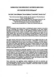
score is above the mean. If μ and σ are not known they can be estimated from the dataset. Each feature will have the mean value 0 after z-score normalization. The unit of each value will be the number of standard deviations which will be far away from the mean. Z-score normalization will give exact values to the small values of σ. In this paper, z-score normalization is applied to scale the influent parameters and thus helps tp improve the prediction of COD level. Feature Selection: Feature selection allows reducing the feature space and helps in improving the accuracy by reducing training time. A Feature Selection Algorithm (FSA) is a computational solution which can be motivated by the definition of relevance (Ladha and Deepa., 2011).The main goal of FSA is to determine the relevant features of the dataset based on relevance. Genetic Algorithms is employed in the proposed method for feature selection. Genetic Algorithms (GA) are search algorithms which are based on the concepts of natural selection and natural genetics. Genetic algorithm was enlarged to replicate some of the processes examined in natural evolution. The genetic algorithm searches along with a population of points and works with a coding of parameter set, instead of the parameter values. It utilizes objective function information without any gradient information (Van et al., 2005). Hence the transition scheme of the genetic algorithm is probabilistic. GA also provides means to search irregular space and thus used for a variety of parameter estimation, function optimization, and machine learning applications. Because of these features genetic algorithm is employed in the proposed work for feature selection to improve the quality and speed in determining COD effluent level present in the wastewater. The procedure for genetic algorithm is described as follows: Genetic Algorithm Formulate initial population Randomly initialize population Repeat Evaluate objective function Find fitness function Apply genetic operators Reproduction Crossover Mutation Until stopping criteria Fig. 1 show the basic operations involved in the GA method. The generation is subdivided into a selection phase and recombination phase. During the selection phase, strings are assigned into adjacent slots. Selection

Current Population

Crossover

After Selection

Mutation

After Crossover

Fig. 1: Basic Operation in GA

121

New Population

Aust. J. Basic & Appl. Sci., 7(10): 119-126, 2013

In the first step of GA, pseudo random generators whose individual signifies a possible solution produce a population having P individuals. This is a demonstration of solution vector in a solution space called initial solution. This guarantees the search to be robust and unbiased since it starts from wide range of points in the solution space. Individual members of the population are assessed to determine the objective function value in the next step. The exterior penalty function process is employed to transform a constrained optimization problem to an unconstrained one. Then, the objective function is mapped into a fitness function that computes a fitness value for each member of the population. Consider the maximization problem Maximize 𝑓𝑓(𝑥𝑥) = 𝑥𝑥𝑖𝑖𝑙𝑙 ≤ 𝑥𝑥𝑖𝑖 ≤ 𝑥𝑥𝑖𝑖𝑢𝑢 , 𝑖𝑖 = 1,2, … . 𝑛𝑛

(2)

Where 𝑥𝑥𝑖𝑖𝑙𝑙 and 𝑥𝑥𝑖𝑖𝑢𝑢 are the lower and upper bound of the variable. According to the following linear mapping rule, the string can be found to represent a point in the search space. 𝑥𝑥𝑖𝑖 = 𝑥𝑥𝑖𝑖𝑙𝑙 +

𝑥𝑥 𝑖𝑖𝑢𝑢 − 𝑥𝑥 𝑖𝑖𝑙𝑙 2𝛽𝛽 −1

∑𝛽𝛽𝑗𝑗=0 𝛾𝛾𝑗𝑗 2𝑗𝑗

(3)

The variable 𝑥𝑥𝑖𝑖 is coded with sub-string 𝑠𝑠𝑖𝑖 of length. The decoded value of a binary sub-string 𝑠𝑠𝑖𝑖 is 𝛽𝛽 computed as ∑𝑗𝑗 =0 𝛾𝛾𝑗𝑗 2𝑗𝑗 where 𝑠𝑠𝑖𝑖 ∈ (0,1) and the string s is represented as𝑠𝑠𝛽𝛽 −1 , 𝑠𝑠𝛽𝛽 −2 … … 𝑠𝑠2 , 𝑠𝑠1 , 𝑠𝑠0 . The length of a sub-string representing a variable depends on the desired accuracy in that variable. It varies with the desired precision of the results, such that longer the string length, the more will be the accuracy. The relationship between string length 𝛽𝛽and precision 𝛼𝛼 is given by (𝑥𝑥𝑖𝑖𝑢𝑢 − 𝑥𝑥𝑖𝑖𝑙𝑙 ) 10𝛼𝛼 ≤ �2𝛽𝛽 − 1�

(4)

The corresponding point x = (x1 , x2 , … . xN )T can be found if the coding of the variables is complete. The function value at the point x can also be calculated by substituting x in the given objective function f(x). A fitness function F (i) is obtained from the objective function and used in consecutive genetic operations. Fitness is a measure of the reproductive efficiency of chromosomes. Fitness function is used to allocate reproductive attributes to the individuals in the population and an individual which has higher fitness value will have higher probability of being selected as candidates for further assessment (Michalewicz., 1999). Fitness function can be considered to be the same as the objective function for maximization problems i.e. F(i) = O(i). In case of minimization problems, it is necessary to map the essential natural objective function to fitness function form inorder to create non-negative values in all the cases and to reproduce the comparative fitness of individual string. 𝐹𝐹(𝑥𝑥) =

1

(5)

1+𝑓𝑓(𝑥𝑥)

This transformation does not change the position of the minimum, but it converts a minimization problem to an equivalent maximization problem. It can be also done using the following equation, 𝑂𝑂(𝑖𝑖)𝑃𝑃

𝐹𝐹(𝑖𝑖) = 𝑉𝑉 − ∑𝑝𝑝

𝑖𝑖=1

(6)

𝑂𝑂(𝑖𝑖)

Where O(i) is the objective function value of ith individual of the population size and V is a large value to ensure non-negative fitness values. Reproduction, crossover, and mutation are the three operators to create a new population of points. The function of these operators is to generate new solution vectors by selection, alteration or combination of the current solution vectors which has shown to be good temporary solutions. The new population is estimated and tested till termination. Reproduction (or selection) operator creates several reproductions of improved strings in a new population. A crossover operator is used to recombine two strings to get a better string. Recombination process produces dissimilar individuals in the successive generations by joining substance from two individuals of the previous generation. Mutation inserts new information in a random way to the genetic search process and eventually assists to evade getting trapped at local optima. Application of these operators on the current population creates a new population which is used to generate subsequent populations. Genetic algorithm with these three operators finds the best solution to the problem. A fitness or objective function is determined by decoding the strings and is calculated in every generation.. It completes one cycle of genetic algorithm called a generation. In every generation, the improved solution is stored as the best solution which is repeated till convergence.

122

Aust. J. Basic & Appl. Sci., 7(10): 119-126, 2013

Prediction of COD: COD test is a common water quality test used to indirectly measure the total amount of organic compounds in a water sample using a strong oxidizing agent such as potassium dichromate. A high COD value indicates a high concentration of organic matter in the water sample. Back Propagation Neural Network (BPN) is the training technique used in this research work for the prediction of COD level in wastewater. Evaluating the error function using the validation subset data, independently and then compares the performance of the networks. The testing subset data are then used to measure the generalization of the network. The processing Steps are as follows: 1. Set up the network based on the problem domain. 2. Weights Wij are randomly generated . 3. Feed a training set, [X1,X2,….Xn], into BPN. 4. The weighted sum is computed and the transfer function is applied on each node in each layer. Feeding the transferred data to the next layer until the output layer is reached. 5. The predicted output is compared with the desired output and an error is computed for each unit. 6. The error is back propagated. 7. Each unit in hidden layer receives only a portion of total errors and these errors then feedback to the input layer. 8. Step 4 is repeated until the error is very small. 9. Step 3 is repeated again for another training set. A Modified LM algorithm is used for training the neural network. Considering performance index is 𝐹𝐹(𝑤𝑤) = 𝑒𝑒 𝑇𝑇 𝑒𝑒 using the Newton method the equation obtained is as follows:

𝑊𝑊𝐾𝐾+1 = 𝑊𝑊𝐾𝐾 − 𝐴𝐴−1 𝐾𝐾 . 𝑔𝑔𝐾𝐾

(7)

𝐴𝐴𝑘𝑘 = ∇2 𝐹𝐹(𝑤𝑤)|𝑤𝑤=𝑤𝑤 𝑘𝑘 𝑔𝑔𝑘𝑘 = ∇𝐹𝐹(𝑤𝑤)|𝑤𝑤=𝑤𝑤 𝑘𝑘 [∇𝐹𝐹(𝑤𝑤)]𝑗𝑗 =

𝜕𝜕𝜕𝜕 (𝑤𝑤) 𝜕𝜕𝑤𝑤 𝑗𝑗

(8) (9)

= 2 ∑𝑁𝑁 𝑖𝑖=1 𝑒𝑒𝑖𝑖 (𝑤𝑤).

𝜕𝜕𝑒𝑒 𝑖𝑖 (𝑤𝑤 )

The gradient can be written as:

(10)

𝜕𝜕𝑤𝑤 𝑗𝑗

∇𝐹𝐹(𝑥𝑥) = 2𝐽𝐽𝑇𝑇 𝑒𝑒(𝑤𝑤) Where

𝜕𝜕𝑒𝑒11 𝜕𝜕𝑒𝑒11

(11) 𝜕𝜕𝑒𝑒11

⎡ 𝜕𝜕𝑤𝑤 1 𝜕𝜕𝑤𝑤 2 … 𝜕𝜕𝑤𝑤 𝑁𝑁 ⎤ ⎢ 𝜕𝜕𝑒𝑒21 𝜕𝜕𝑒𝑒21 𝜕𝜕𝑒𝑒21 ⎥ ⎢ 𝜕𝜕𝑤𝑤 1 𝜕𝜕𝑤𝑤 2 … 𝜕𝜕𝑤𝑤 𝑁𝑁 ⎥ . ⎥ 𝐽𝐽(𝑤𝑤) = ⎢ ⎢ ⎥ . ⎢ ⎥ . ⎢𝜕𝜕𝑒𝑒𝐾𝐾𝐾𝐾 𝜕𝜕𝑒𝑒𝐾𝐾𝐾𝐾 𝜕𝜕𝑒𝑒𝐾𝐾𝐾𝐾 ⎥ … ⎣ ⎦ 𝜕𝜕𝑤𝑤 1 𝜕𝜕𝑤𝑤 2

(12)

𝜕𝜕𝑤𝑤 𝑁𝑁

𝐽𝐽(𝑤𝑤)is called the Jacobian matrix. Then, the Hessian matrix is to be found. The k, j elements of the Hessian matrix yields as: 𝑁𝑁 𝜕𝜕𝑒𝑒𝑖𝑖 (𝑤𝑤) 𝜕𝜕𝑒𝑒𝑖𝑖 (𝑤𝑤) 𝜕𝜕 2 𝑒𝑒𝑖𝑖 (𝑤𝑤) [∇2 𝐹𝐹(𝑤𝑤)]𝑘𝑘,𝑗𝑗 = 2 � � + 𝑒𝑒𝑖𝑖 (𝑤𝑤). � 𝜕𝜕𝑤𝑤𝑘𝑘 𝜕𝜕𝑤𝑤𝑗𝑗 𝜕𝜕𝑤𝑤𝑘𝑘 𝜕𝜕𝑤𝑤𝑗𝑗 𝑖𝑖=1 The Hessian matrix can then be signified as follows: ∇2 𝐹𝐹(𝑤𝑤) = 2𝐽𝐽𝑇𝑇 (𝑊𝑊). 𝐽𝐽(𝑊𝑊) + 𝑆𝑆(𝑊𝑊)

(13)

2 𝑆𝑆(𝑤𝑤) = ∑𝑁𝑁 𝑖𝑖=1 𝑒𝑒𝑖𝑖 (𝑤𝑤). ∇ 𝑒𝑒𝑖𝑖 (𝑤𝑤)

(14)

123

Aust. J. Basic & Appl. Sci., 7(10): 119-126, 2013

If S(w) is small assumed, the Hessian matrix can be approximated as:

∇2 𝐹𝐹(𝑤𝑤) ≅ 2𝐽𝐽𝑇𝑇 (𝑤𝑤)𝐽𝐽(𝑤𝑤)

(17)

Using equations (11) and (17), the Gauss-Newton method is obtained as follows:

𝑊𝑊𝑘𝑘+1 = 𝑊𝑊𝑘𝑘 − [2𝐽𝐽𝑇𝑇 (𝑤𝑤𝑘𝑘 ) ∙ 𝐽𝐽(𝑤𝑤𝑘𝑘 )]−1 2𝐽𝐽𝑇𝑇 (𝑤𝑤𝑘𝑘 )𝑒𝑒(𝑤𝑤𝑘𝑘 ) ≅ 𝑊𝑊𝑘𝑘 − [𝐽𝐽𝑇𝑇 (𝑤𝑤𝑘𝑘 ) ∙ 𝐽𝐽(𝑤𝑤𝑘𝑘 )]−1 𝐽𝐽𝑇𝑇 (𝑤𝑤𝑘𝑘 )𝑒𝑒(𝑤𝑤𝑘𝑘 )

(18)

The advantage of Gauss-Newton is that it does not need computation of second derivatives. The problem in the Gauss-Newton method is the matrix 𝐻𝐻 = 𝐽𝐽𝑇𝑇 𝐽𝐽 may not be invertible which can be overcome by using the following modification. Hessian matrix can be written as: 𝐺𝐺 = 𝐻𝐻 + 𝜇𝜇𝜇𝜇

(19)

Suppose that the eigen values and eigenvectors of H are {𝜆𝜆1 , 𝜆𝜆2 , … … . , 𝜆𝜆𝑛𝑛 } and {𝑧𝑧1 , 𝑧𝑧2 , … … . , 𝑧𝑧𝑛𝑛 }.Then:

𝐺𝐺𝑧𝑧𝑖𝑖 = [𝐻𝐻 + 𝜇𝜇𝜇𝜇]𝑧𝑧𝑖𝑖 = 𝐻𝐻𝑧𝑧𝑖𝑖 + 𝜇𝜇𝑧𝑧𝑖𝑖 = 𝜆𝜆𝑖𝑖 𝑧𝑧𝑖𝑖 + 𝜇𝜇𝑧𝑧𝑖𝑖 = (𝜆𝜆𝑖𝑖 + 𝜇𝜇)𝑧𝑧𝑖𝑖

(20)

As a result, the eigenvectors of G are the identical as the eigenvectors of H, and the eigen values of 𝐺𝐺 are (𝜆𝜆𝑖𝑖 + 𝜇𝜇). The matrix G is positive definite by enhancing μ until (𝜆𝜆𝑖𝑖 + 𝜇𝜇) > 0 for all i therefore the matrix will be invertible. This leads to LM algorithm: 𝑤𝑤𝑘𝑘+1 = 𝑤𝑤𝑘𝑘 − [𝐽𝐽𝑇𝑇 (𝑤𝑤𝑘𝑘 )𝐽𝐽(𝑤𝑤𝑘𝑘 ) + 𝜇𝜇𝜇𝜇]−1 𝐽𝐽𝑇𝑇 (𝑤𝑤𝑘𝑘 )𝑒𝑒(𝑤𝑤𝑘𝑘 )

(21)

∆𝑤𝑤𝑘𝑘 = [𝐽𝐽𝑇𝑇 (𝑤𝑤𝑘𝑘 )𝐽𝐽(𝑤𝑤𝑘𝑘 ) + 𝜇𝜇𝜇𝜇]−1 𝐽𝐽𝑇𝑇 (𝑤𝑤𝑘𝑘 )𝑒𝑒(𝑤𝑤𝑘𝑘 )

(22)

𝜇𝜇 = 0.01𝑒𝑒 𝑇𝑇 𝑒𝑒

(23)

As known, learning parameter, μ is illustrator of steps of real output movement to preferred output. In the standard LM method, μ is a steady number. This work modifies LM method using μ as:

Where e is a 𝑘𝑘 × 1 matrix therefore 𝑒𝑒 𝑇𝑇 𝑒𝑒 is a 1 × 1 therefore [𝐽𝐽𝑇𝑇 𝐽𝐽 + 𝜇𝜇𝜇𝜇]is invertible. Therefore if actual output is far than desired output or correspondingly, errors are large so it converges to desired output with large steps. Similarly when measurement of error is small subsequently actual output approaches to desired output with soft steps therefore error oscillation reduces greatly. The influent COD levels which are the controlling parameters of anaerobic reactor were considered as the input parameters. The model was trained with BPN using modified LM algorithm to recognize these input parameters in order to predict the corresponding effluent level of COD as output parameters. The tansig and purelin were the activation functions used in the hidden layer and output layer respectively. The model was developed by using Matlab software. The parameter for learning rate is 0.04, the epoch is 150, and the error goal is about 1e-5. Thus, the model was trained using BPN training algorithm and it was found that the network model learnt to adjust the weights to predict the target outputs. Experimental Results: Daily records from the operation of an anaerobic filter treating agro-food wastewater during a period of 6 months were obtained. The raw data relate to the anaerobic digester and each sample comprises three variables. The importance of the wastewater treatment system is continuously growing, as sustainable development of the modern society is concerned on the health of the environment. In the anaerobic data, the total discernible samples based on the effluent COD when using COD, volatile suspended solid, total suspended solid, flow rate , OLR, HRT, pH, alkanity, etc., as inputs in the crude supply stream from the dataset of an anaerobic treatment system is found to be treated up to 80%. Two statistical indices are used in order to evaluate the performance of the proposed model: Mean Square Error (MSE), Mean Absolute Error (MAE) and Regression (R) values that are derived in statistical calculation of observation in model output predictions can be defined as:

124

Aust. J. Basic & Appl. Sci., 7(10): 119-126, 2013

MSE = ∑𝑁𝑁 𝑖𝑖=1 R=

(𝑥𝑥−𝑦𝑦)2

(25)

𝑁𝑁

∑(𝑥𝑥−𝑥𝑥)(𝑦𝑦−𝑦𝑦) ∑(𝑥𝑥−𝑥𝑥)

(26)

2

Table 1 and table 2 shows that the results obtained from the prediction system to predict the effluent COD level in wastewater using BPN with Z-score and Genetic Algorithm. Table 1: The performance of the predicting system based on regression, Mean square error and Mean absolute error values using GA-BPN Method Regression MSE MAE With z-score normalization & without 0.511 60.12 12.120 Feature Selection With z-score normalization & with GA 0.923 49.28 5.48 Feature Selection Table 2: Performance of the Prediction system based on training time and testing time using GA-BPN Method Training time (secs) Testing time (secs) With z-score normalization & without Feature Selection 26.218 9.431 With z-score normalization & with GA Feature Selection 11.141 0.803

It is observed from the above table 1, the experimental results shows that the regression, MSE and MAE are 0.923, 49.28 and 5.48 respectively. The performance of prediction system using BPN with z-sore normalization and GA is better than without normalization and feature selection. It is observed from the above table 2, that the z-sore normalization, GA with BPN has taken minimum training time and testing time. Genetic Algorithm is used to select only required influent parameters to predict the COD level. From the normalized 10 influent parameters, 7 influent features were selected by GA. Hence BPN with GA and Z-score is found to be an attractive option in predicting the effluent levels with more accuracy. Conclusion: The Application of Intelligent Computing Systems like Back Propagation Neural Network (BPN) to an anaerobic filter containing cheese dairy wastewaters led to develop a model that analyzed the various input variables and also predict the effluent COD. The Z-score normalization technique helps to improve the training of influent parameters by BPN model. The BPN model developed using Modified Levenberg – Marquardt (MLM) algorithm with genetic algorithm as a feature selection process provided good prediction of effluent COD level covering a range of data for training and testing purposes on comparing the results. The performance of the network was found satisfactory based on regression, MSE and MAE when developed using GA and BPN with MLM algorithm as it showed accurate prediction of COD level. REFERENCES Esposito, G., L. Frunzo, A. Giordano, F. Liotta, A. Panico, F. Pirozzi, 2012. Anaerobic co-digestion of organic wastes. Rev. Environ. Sci. Biotechnol., 11: 325-341. Hamed, M.M., M.G. Khalafallah, E.A. Hassanien, 2004. Prediction of wastewater treatment plant performance using artificial neural networks. Environmental Modeling Soft., 19: 919-928. Huang, M., Ma. Yongwen, J. Wana, H. Zhang, Y. Wang, Y. Chen, C. Yoo, W. Guo, 2011. A hybrid genetic – Neural algorithm for modeling the biodegradation process of DnBP in AAO system. Bioresource Technology, 102: 8907-8913. Jayalakshmi, T., A. Santhakumaran, 2011. Statistical Normalization and Back Propagation for Classification. International Journal of Computer Theory and Engineering, 3(1): 1793-820. Ladha, L., T. Deepa, 2011. Feature Selection Methods and Algorithms. International Journal on Computer Science and Engineering, 3(5): 0975-3397. Leita, R.C., A.C. Haandel, G. Zeeman, G. Lettinga, 2006. The effects of operational and environmental variations on anaerobic wastewater treatment system. A review. Bio-resource Technology, 9: 1105-1118. Lippmann, R.P., 1987. An Introduction to Computing with Neural Nets, IEEE ASSP Magazine. Michalewicz, Z., 1999. Genetic Algorithms + Data Structures = Evolution Programs, Springer-Verlag, 3rd edition. Parthiban, R., L. Parthiban, 2012. Back propagation Neural network modeling approach in the anaerobic digestion of wastewater treatment. International Journal of Environmental Sciences, 2(4). Rajagopal, R., N.M.C. Saady, M. Torrijos, J.V. Thanikal, Y-T. Hung, 2013. Sustainable Agro-Food Industrial Wastewater Treatment Using High Rate Anaerobic Process. Water, 5: 292-311.

125

Aust. J. Basic & Appl. Sci., 7(10): 119-126, 2013

Rajinikanth, R., R. Ganesh, Pradeep Kumar, J.V. Thanikald, 2013. High rate anaerobic filter with floating supports for the treatment of effluents from small-scale agro-food industries. Desalination and Water Treatment., 4: 183-190. Scheel, I., M. Aldrin, I.K. Glad, R. Sorum, H. Lyng, A. Frigessi, 2005. The influence of missing value imputation on detection of differentially expressed genes from microarray data. Bioinformatics, 21: 4272-4279. Van Dijck, G., M.M. Van Hulle, M. Wevers, 2005. Genetic Algorithm for Feature Subset Selection with Exploitation of Feature Correlations from Continuous Wavelet Transform: a real-case Application. World Academy of Science, Engineering and Technology, 1. Wastewater Treatment Manuals Primary, Secondary and Tertiary Treatment, 1997. Published by the Environmental Protection Agency. ISBN: 1899965467.

126