Improving the Performance of a Genetic Algorithm Using a Variable

Improving the Performance of a Genetic Algorithm Using a Variable-Reordering Algorithm Eduardo Rodriguez-Tello1 and Jose Torres-Jimenez2 1

LERIA, Université d’Angers 2 Boulevard Lavoisier, 49045 Angers, France [email protected] 2 ITESM Campus Cuernavaca, Computer Science Department. Av. Paseo de la Reforma 182-A. 62589 Temixco Morelos, Mexico [email protected]

Abstract. Genetic algorithms have been successfully applied to many difficult problems but there have been some disappointing results as well. In these cases the choice of the internal representation and genetic operators greatly conditions the result. In this paper a GA and a reordering algorithm were used for solve SAT instances. The reordering algorithm produces a more suitable encoding for a GA that enables a GA performance improvement. The attained improvement relies on the building-block hypothesis, which states that a GA works well when short, low-order, highly-fit schemata (building blocks) recombine to form even more highly fit higher-order schemata. The reordering algorithm delivers a representation which has the most related bits (i.e. Boolean variables) in closer positions inside the chromosome. The results of experimentation demonstrated that the proposed approach improves the performance of a simple GA in all the tests accomplished. These experiments also allow us to observe the relation among the internal representation, the genetic operators and the performance of a GA.

1

Introduction

A genetic algorithm (GA) is based on three elemental parts: an internal representation, an external evaluation function and an evolutionary mechanism. The GA is considered to be successful if a population of highly fit individuals evolves as a result of iterating this procedure. The GAs, unlike other optimization algorithms, use in the search process of a solution not only the fitness values, but also the similarities that exist between certain patterns with high aptitude, that is to say, they change the emphasis of searching complete strings by discovering partially adapted strings. Given this fact it is useful to study the similarities of these patterns along with its corresponding fitness values, and specially to investigate the structural correlations of

strings with exceptional fitness values. Formally, the similarities between strings are defined by means of a schema. A schema (on the binary alphabet, this does not mean lost of generality) is a string of the following type: (a1 , a2 , ..., ai , ..., al ), ai ∈ {0, 1, ∗}. The character “∗” is used for representing a wildcard which can take the values 0 or 1. A schema describes a subspace of strings [12]. For example S1 = (11∗00∗) is a schema in a population of strings with length k = 6 which represents the strings: 111001, 111000, 110001, 110000. The schema’s order o(S), can be defined as the length of the string minus the total number of wildcard characters, in the previous example o(S1 ) = 4; and the schema’s length δ(S) is the distance between the two, non wildcard, most separated characters of the schema (δ(S1 ) = 4). Given that a string is an instance of 3l possible schemata, where l is the length of the string, when its fitness value is verified, it is also derived an important amount of implicit information related with its schemata. Holland called this fact implicit parallelism[19], because the searching process is directed simultaneously in many hyperplanes of the search space. The schemata theorem, which is believed to be a primary source of the GA’s search power, states that a GA works well when short, low-order, highly-fit schemata (building blocks) recombine to form even more highly fit higher-order schemata. In this sense when examining GA hardness it is important to realize that the hardness is essentially due to the internal representation of the search space, and the way genetic operators act upon it [28]. For this reason the representation of a problem must be designed in such a way that the gene interaction (epistasis) is kept as low as possible and the building blocks may form to guide the convergence process towards the global optimum. In an internal representation each locus (bit within the chromosome) discriminates between certain subsets of the search space. Only in one extreme case (zero epistasis, [6]), all loci are of equal importance. Most often, though, certain loci are more important than others in that they discriminate between larger chromosome chunks. Or, correlations between different loci are explicitly or implicitly present. Ideally we would like to order the loci by their discriminating power, and we would like correlated loci to be grouped together. In this paper an algorithm which tries to achieve this is presented. This algorithm is implemented by a simulated annealing algorithm (SA), which transforms the representation of the problem by reordering its variables in such a way that the most related ones can be placed in closer positions inside the chromosome. The rest of this paper is organized as follows: Section 2, presents a historical resume of the GAs performance on the satisfiability problem. In section 3, a detailed description of the GA representation issue for the satisfiability problem is presented. Section 4 focuses on the proposed reordering algorithm and its implementation details. In section 5, the experimental results and comparisons are presented. Finally, in last section, the conclusions of this work are discussed.

2

GAs and the Satisfiability Problem

We are specially interested in applying GAs to the satisfiability (SAT) problem given its great importance in computer science both in theory and in practice. In theory, SAT was the first problem which has been shown to be NP-complete [4]. In practice, it has many applications in different research fields such as planning, formal verification, and knowledge representation; to mention only some. The SAT problem involves finding an assignment to a set of Boolean variables x1 , x2 , ..., xN that satisfies a set of constraints represented by a well-formed Boolean formula in CNF format F : BN → B, B = {0, 1}, i.e., a conjunction of clauses, each of which is a disjunction of variables. If such assignment exists the instance is called satisfiable and unsatisfiable otherwise. Due to its theoretical and practical relevance the SAT problem has been extensively studied and many exact and heuristic algorithms have been introduced. Theoretically, exact methods are able to find the solution, or to prove that no solution exists provided that no time constraint is present. However, given the combinatorial nature of the problem, they have an exponential wortcase complexity. In contrast heuristic algorithms can find solutions to satisfiable instances quickly, but they do not guarantee to give a definitive answer to all problem instances. Existing heuristic algorithms for SAT are essentially based on local search methods [1, 27] and evolutionary strategies [20, 8]. Even though the GAs have been successfully applied to many NP-complete problems, some disappointing results question the ability of GAs to solve SAT. De Jong and Spears proposed a classical GA for SAT and concluded that their GA could not outperform highly tuned, problem-specific algorithms [20]. This result was confirmed experimentally in [9], they reported scarce performance of classical GAs when compared with local search methods. In addition, Rana and Whitley showed pure GAs being unsuitable for the MAXSAT fitness function, which counts the number of satisfied clauses, because the corresponding domain contains misleading low-order schema information, and the search space tends to result in similar schema fitness averages [26]. Recent results showed that GAs can nevertheless yield good results for SAT if equipped with additional techniques. These techniques include adaptive fitness functions, problem-specific genetic operators, and local optimization [8, 9, 24, 13]. We have strong reasons to think that the negative results in the use of classical GA for SAT is caused by the effect of an inappropriate representation. In the next section, the representation issue will be described in greater detail.

3

The Representation Issue

SAT has a natural representation in GAs: binary strings of length N in which the i − th bit represents the truth value of the i − th Boolean variable present in the SAT formula, surprisingly, no efficient classical genetic algorithm has been found yet using this representation alone [14]. We have strong reasons to think that this poor performance is caused by the effect of an inappropriate representation.

(a)

(b)

(c)

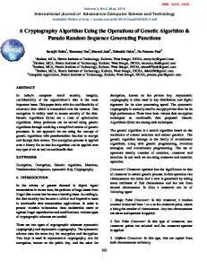
Fig. 1. (a) Closeness’ graph for Dubois50.cnf original variable-ordering. (b) Closeness’ graph for the Dubois50.cnf with a bad variable-ordering. (c) Closeness’ graph for the Dubois50.cnf with a good variable-ordering.

An easy extension of the building block hypothesis [12] is that a chromosome representation must satisfy the fact that related variables are coded in closer positions in the chromosome representation. As a consequence, it is very desirable that two variables that participate in the same clause appear close in the chromosome representation, and through a variable reordering algorithm it is possible to control the “closeness” of SAT instance related variables. A graphical view of variables’ “closeness” can be constructed using the graph of a binary matrix R s.t. Ri,j = 1 if the i − th variable appears related with the j − th variable at least one time in a clause and (i < j), and otherwise Ri,j = 0. The graph of the binary matrix R contains a dot in position (i, j) just in case Ri,j = 1, The SAT instance Dubois50.cnf 3 will be used for presenting graphs that correspond to: a) the original variable-ordering, b) a bad variable-reordering, and c) a good variable-reordering (a good reordering means that related variables appear in closer positions within the chromosome representation saw by a GA). In Figure 1(a) the graph that corresponds to the original ordering of the SAT instance Dubois50.cnf is presented, in this ordering two related variables are separated at most 101 positions (i.e. if the two related variables are i and j, then max(abs(i − j)) = 101). In Figure 1(b) the graph corresponding to a bad reordering for the SAT instance Dubois50.cnf is presented, in this case two related variables are separated at most 149 positions (this corresponds to a worst reordering given that two related variables appear in the most far positions within the chromosome, i.e. first chromosome position and last chromosome position). In Figure 1(c) the graph corresponding to a good reordering is presented, in this case two related variables are separated at most 10 positions (i.e. max(abs(i − j)) = 10, where i and j are two related variables). As a general 3

It consists of 150 variables and http://www.satlib.org/benchm.html

400

clauses

and

can

be

found

at

guideline if the dots appear near the main diagonal of the closeness’ graph that indicates a variable-ordering, it implies that the representation is good.

4

The Reordering Algorithm

The proposed algorithm has as input a CNF instance, this CNF formula is then converted into a weighted graph, where each variable is represented by a node, and each weighted edge denotes how many times the variable i is related with the variable j. (see Figure 2(a)). A bandwidth minimization algorithm [30] is applied to the resulting weighted graph to produce a more suitable ordering of the weighted graph nodes. This ordering is translated back into an ordering of variables in the original CNF instance. After that, the preprocessed CNF formula can be used as input to a classical GA (see Figure 2(b)). Note that this preprocessing algorithm does not change the original problem only rename its variables.

(a)

(b)

Fig. 2. (a) Weighted graph corresponding to the SAT instance: (∼ A ∨ B∨ ∼ C) ∧ (A ∨ B ∨ E) ∧ (A ∨ E∨ ∼ F ) ∧ (∼ B ∨ D∨ ∼ G) (b) Reordering variable heuristic based on a Bandwidth Minimization Algorithm.

4.1

Some Important Definitions

There are essentially two ways in which the bandwidth minimization problem (BMP) can be approached, whether as a graph or as a matrix. The equivalence of a graph and a matrix is made clear by replacing the nonzero entries of the matrix by 10 s and interpreting the result as the adjacency matrix of a graph. The Matrix Bandwidth Minimization Problem seems to have been originated in the 1950’s when structural engineers first analyzed steel frameworks by computer manipulation of their structural matrices [22, 23]. In order that operations like inversion and finding determinants take the least time as possible, many

efforts were made to discover an equivalent matrix in which all the nonzero entries would lay within a narrow band near the main diagonal (hence the term “bandwidth”) [3]. The BMP for graphs (BMPG) was proposed independently by Harper [18] and Harary [17]. This can be defined as finding a labeling for the vertices of a graph, where the maximum absolute difference between labels of each pair of connected vertices is minimum. Formally, Let G = (V, E) be a finite undirected graph, where V defines the set of vertices (labeled from 1 to N ) and E is the set of edges. And a linear layout τ = {τ1 , τ2 , ..., τN } of G is a permutation over {1, 2, ...N }, where τi denotes the label of the vertex that originally was identified with the label i. The bandwidth β of G for a layout τ is: βτ (G) = M ax{u,v}∈E |τ (u) − τ (v)|.

(1)

Then the BMPG can be defined as finding a layout τ for which βτ (G) is minimum. The first work that helped to understand the computer complexity of the BMPG, was developed by Papadimitriou, who demonstrated that the decision problem associated to the BMPG is a NP-complete problem [25]. Later, it was demonstrated that the BMPG is NP-complete even for trees with a maximum degree of three [10]. There are several algorithms reported to solve the BMPG, they can be divided into two classes: exact and approximate algorithms. Exact algorithms, guaranteed always to discover the optimal bandwidth, example of exact algorithm is the one published by Gurari and Sudborough [15], it solves the BMPG in O(N k ) steps, where k is the bandwidth searched for that graph. Approximate algorithms are best known as approximate in the sense that they do not guarantee to find the actual bandwidth of the graph, examples of this sort of algorithms are [5, 11, 16]. All algorithms mentioned in last paragraph use as a measure of the quality for a solution β. The only reported exceptions are: Dueck’s work in which not only β is used, but he also takes into account differences among adjacent vertices close to β [7], and [30] where a new measure, namely γ, is proposed. The advantage of this new measure is the ability to distinguish even the smallest improvements that not necessarily lower the value of β. Based in this previously reported work, we have implemented an algorithm for improving the representation of a problem used for a GA. The new representation produced by our algorithm satisfies the condition that the most related variables of the problem are placed in closer positions inside the chromosome. Next the implementation details of this algorithm are presented. 4.2

Implementation Details

The reordering algorithm approximates the bandwidth of a graph G by examining randomly generated layouts τ of G. These new layouts are generated by

interchanging a pair of distinct labels of the set of vertices V . This interchanging operation is called a move. The reordering algorithm begins initializing some parameters as the temperature, the maximum number of accepted moves at each temperature, and the cooling rate. The algorithm continues by randomly generating a move and then calculating the change in the cost function for the new labelling of the graph. If the cost decreases then the move is accepted. Otherwise, it is accepted with probability P (∆C) = e−∆C/T where T is the temperature and ∆C is the increase in cost that would result from a particular move. The next temperature is obtained by using the relation Tn = Tn−1 ∗ 0.85. The minimum bandwidth of the labellings generated by the algorithm up that point is stored. The number of accepted moves is counted and if it falls below a given limit then the system is frozen. The parameters of the SA algorithm were chosen experimentally, and taking into account some related work reported in [21, 30, 29]. It is important to remark that the maximum number of accepted moves at each temperature, depends directly on the number of edges of the graph, because more moves are required for denser graphs. Next the reordering algorithm is presented: Procedure SA(G) Set initial temperature (T) and all the parameters Generate an initial random labelling for G Calculate its bandwidth (old) Repeat Repeat Generate a random move Calculate its bandwidth (new) If ((new-old) < 0) Or (Random[0,1) < Exp(-(new-old)/T)) Accept the move If (new < old) old = new EndIf EndIf Until pre-defined number of iterations for this temperature Reduce the temperature (Tn = Tn−1 ∗ 0.85) Until temperature > minimum temperature EndSA

5

Experimental Results

To evaluate the effectiveness the proposed reordering algorithm, a classic GA was implemented. Its internal representation is based on binary strings of length N in which the i − th bit represents the truth value of the i − th Boolean variable of the problem. This chromosome definition has the following advantages: It is of fixed length, binary, context independent in the sense that the meaning of one bit is unaffected by changing the value of other bits, and permits the use of

classic genetic operators defined by Holland [19], which have strong mathematical foundations. Recombination is done in the standard way using the two-point crossover operator, and the bit flipping operator. The former has been applied at a 70% rate, and the latter at a 0.01% rate (these parameter values were adjusted through experimentation). Selection operator is similar to the tournament selection reported in [2]; randomly three elements of the population are selected and the one with the better fitness is chosen. The choice of the fitness function is an important aspect of any genetic optimization procedure. Firstly, in order to efficiently test each individual and determine if it is able to survive, the fitness function must be as simple as possible. Secondly, it must be sensitive enough to locate promising search regions on the space of solutions. Finally, the fitness function must be consistent: a solution that is better than others must have a better fitness value. For the SAT problem the fitness function used is the simplest and most intuitive one, the fraction of the clauses that are satisfied by the assignment. More formally:

M

f (chromosome) =

1 X f (Ci ) M i=1

(2)

Where M is the number of clauses in the problem and the contribution of each clause f (Ci ) is 1 if the clause is satisfied and 0 otherwise. All the experiments were done using a population size fixed at: b1.6 ∗ N c, where N is the number of variables in the SAT problem. The termination condition used for this algorithm is either when a solution that satisfies all the clauses is found, or when the maximum number of 500 generations is reached. The proposed reordering algorithm was tested on several classes of satisfiable and unsatisfiable benchmark instances as those of the second DIMACS challenge and flat graph coloring instances. They are easily available from the SATLIB web site4 . For each of the selected instances 40 independent runs were executed, 20 using the reordering algorithm plus the classic GA (R+GA), and 20 solving the problem with the use of the same basic GA. The results reported here, are data averaged over the 20 corresponding runs. Both the reordering algorithm and the GA have been implemented in C programming language and ran into a Pentium 4 1.7 Ghz. with 256 MB of RAM. Table 1 presents the comparison between R+GA and the GA. Data included in this comparison are: name of the formula; number of variables N ; number of clauses M ; βi and βf represent the initial and final bandwidth obtained with the reordering algorithm; the CPU time in seconds used by the reordering algorithm is Tβ . Additionally, for each approach it is presented: the number of satisfied 4

http://www.satlib.org/benchm.html

clauses SC, and the CPU time in seconds T . It is important to remark that the times presented for the combined approach in the column TT otal take into account the CPU time used for the preprocessing algorithm.

Table 1. Comparative results between R+GA and GA.

Formulae aim100-1_6y aim100-2_0y dubois28 dubois29 dubois30 dubois50 flat30-1 flat30-2 pret60-75 pret150-40 pret150-60 pret150-75

N 100 100 84 87 90 150 90 90 60 150 150 150

M 160 200 224 232 240 400 300 300 160 400 400 400

βi 94 96 77 81 87 144 85 81 56 143 140 142

R βf 37 42 9 9 9 10 26 24 10 24 27 23

Tβ 3.1 5.2 1.0 1.0 1.0 2.1 2.2 2.2 1.0 2.1 3.1 3.0

SC 160 200 223 231 239 397 300 300 159 399 399 397

R+GA T TTotal 4.95 8.05 4.36 9.56 2.08 3.08 1.09 2.09 13.35 14.35 1.93 4.03 16.61 18.81 11.44 13.64 1.75 2.75 33.63 35.73 12.75 15.85 35.82 38.82

GA SC T 159 16.81 198 10.11 221 7.25 231 19.89 237 27.81 395 39.94 299 27.41 300 17.82 159 14.67 396 23.84 397 21.31 397 65.76

The results of experimentation presented showed that the combined approach R+GA outperforms the simple GA in all the tests accomplished, not only in solution quality but also in computing time. The set of four satisfiable instances5 used in the experiments were solved by R+GA while only one of them could be solved by GA. Better quality solutions for the R+GA is possible thanks to the representation used by the GA ran after the reordering algorithm. This new representation has two very important characteristics: it keeps the gene interaction as low as possible and promotes the creation of building blocks. Smaller computing time for the R+GA approach is possible because the reordering algorithm is able to find good solutions in reasonable time and also because the GA using the new representation takes less CPU time. This can be clearly appreciated in the Figure 3. It shows the convergence process of the two compared algorithms. The X axis represents CPU time in seconds used by the algorithms, while the Y axis indicates the number of satisfied clauses. It is important to point out that the R+GA curve initiates at the time Tβ , which is the CPU time in seconds consumed in the reordering stage. The behavior of a classic GA ran on the same problem with different bandwidths of the associated graph (Beta) has been explored. In Figure 4 it can be seen that the performance of the GA is better when the bandwidth is low, i.e. the most related variables are placed in closer positions inside the chromosome. Next section presents the conclusions of this work. 5

In Table 1 a

indicates a satisfiable formula.

240

305

235 300

Satisfied Clauses

Satisfied Clauses

230

225

295

290

220

285 215 R + GA GA Solution

R + GA GA 210

280 0

5

10

15

20

25

0

5

10

Seconds

15

20

25

Seconds

(a)

(b)

400

400

395

395

390

390

Satisfied Clauses

Satisfied Clauses

Fig. 3. Average best-so-far curves for R+GA and GA on the problems dubois29 (a) and flat30-2 (b).

385

380

385

380

375 375 370 370 Beta=10 Beta=94 Beta=149

365

0

50

100

150

200

250 300 Generations

(a)

350

400

450

Beta=23 Beta=95 Beta=149

365 500

0

50

100

150

200

250 300 Generations

350

400

450

(b)

Fig. 4. Average best-so-far curves for a classic GA ran with different bandwidths on the problems dubois50 (a) and Pret150-75 (b).

500

6

Conclusions

In this paper a reordering algorithm was used to improve the performance of a classic GA when used to solve SAT problems. This combined approach has been compared versus a simple GA using a set of SAT instances and it outperformed the GA in all the tests accomplished. Additionally it has been observed during the experimentation, that as the size of the problem increases, the advantage to use the proposed reordering algorithm also increases. It allows us to conclude that it pays to make a preprocessing of the problems in order to obtain a more suitable representation. The R+GA method reported in this paper is a preliminary version. Studies are in the way to have a better understanding of its behavior with respect of different classes of SAT instances. Another pending issued is to improve its performance; specially, a better stop criteria. We think that the R+GA method is very promising and worthy to more research. In particular it will be interesting and important to identify the classes of SAT instances where is appropriate to apply our method and if this reordering technique could be used in other kind of problems which will be solved by using GAs.

References 1. Y. Kambayashi B. Cha, K. Iwama and S. Miyasaki, Local search algorithms for partial maxsat, Proceedings of the AAAI 97, July 27-31 1997, pp. 263—268. 2. T. Blickle and L. Thiele, A mathematical analysis of tournament selection, Proceedings of the Sixth ICGA, Morgan Kaufmann Publishers, San Francisco, Ca., 1995, pp. 9—16. 3. P.Z. Chinn, J. Chvatalova, A.K. Dewdney, and N.E. Gibbs, The bandwidth problem for graphs and matrices - a survey, Journal of Graph Theory 6 (1982), no. 3, 223— 254. 4. S. A. Cook, The complexity of theorem proving procedures, 3rd Annual ACM Symposium on the Theory of Computing, 1971, pp. 151—158. 5. E. Cutchill and J. McKee, Reducing the bandwidth of sparse symmetric matrices, Proceedings 24th National of the ACM (1969), 157—172. 6. Y. Davidor, Epistasis Variance: A Viewpont of GA-Hardness, Proceedings of the Second Foundations of Genetic Algorithms Workshop, Morgan Kaufmann, 1991, pp. 23—35. 7. G. Dueck and J. Jeffs, A heuristic bandwidth reduction algorithm, Journal of combinatorial mathematics and computers (1995), no. 18, 97—108. 8. Agoston E. Eiben, Jan K. Van Der Hauw, and Jan Van Hemert, Graph coloring with adaptative evolutionary algorithms, Journal of Heuristics 4 (1998), no. 1, 25— 46. 9. C. Fleurent and J. Ferland, Object-oriented implementation of heuristic search methods for graph coloring, maximum clique, and satisfiability, Second DIMACS Challenge, Special Issue, AMS, Providence, Rhode Island, 1996, pp. 619—652. 10. M.R. Garey, R.L. Graham, D.S. Johnson, and D.E. Knuth, Complexity results for bandwidth minimization, SIAM Journal of Applied Mathematics 34 (1978), 477— 495.

11. N.E. Gibbs, W.G. Poole, and P.K. Stockmeyer, An algorithm for reducing the bandwidth and profile of a sparse matrix, SIAM Journal on Numerical Analysis 13 (1976), 235—251. 12. David E. Goldberg, Genetic Algorithms in Search, Optimization and Machine Learning, Addison-Wesley Publishing Company, Inc., 1989. 13. J. Gottlieb and N. Voss, Improving the performance of evolutionary algorithms for the satisfiability problem by refining functions, Proceedings of the Sixth International Conference on Parallel Problem Solving from Nature (Berlin, Germany), Lecture Notes in Computer Science, vol. Volumen 1917, Springer, 2000, pp. 621— 630. 14. Jens Gottlieb, Elena Marchiori, and Claudio Rossi, Evolutionary algorithms for the satisfiability problem, Evolutionary Computation 10 (2002), no. 1, 35—50. 15. E.M. Gurari and I.H. Sudborough, Improved dynamic programming algorithms for bandwidth minimization and the min-cut linear arrangement problem, Journal of Algorithms 5 (1984), 531—546. 16. J. Haralambides, F. Makedon, and B. Monien, An aproximation algorithm for caterpillars, Journal of Mathematical Systems Theory 24 (1991), 169—177. 17. F. Harary, Theory of graphs and its aplications, Czechoslovak Academy of Science, Prague, 1967, M. Fiedler. 18. L.H. Harper, Optimal assignment of numbers to vertices, Journal of SIAM 12 (1964), 131—135. 19. J. Holland, Adaptation in natural and artificial systems, Ann Arbor: The University of Michigan Press, 1975. 20. Kenneth A. De Jong and William M. Spears, Using genetic algorithms to solve NP-complete problems, Proceedings of the Third ICGA (Fairfax, Virginia), 1989, pp. 124—132. 21. S. Kirkpatrick, C. D. Gelatt, and M. P. Vecchi, Optimization by simulated annealing, Science 220 (1983), 671—680. 22. E. Kosko, Matrix inversion by partitioning - Part 2, The Aeronautical Quarterly (1956), no. 8, 157. 23. R.R. Livesley, The analysis of large structural systems, Computer Journal 3 (1960), no. 1, 34—39. 24. E. Marchiori and C. Rossi, A flipping genetic algorithm for hard 3-SAT problems, Proceedings of Genetic and Evolutionary Computation Conference (San Francisco, California), Morgan Kaufmann, 1999, pp. 393—400. 25. C.H. Papadimitriou, The NP-Completeness of the bandwidth minimization problem, Journal on Computing 16 (1976), 263—270. 26. S. Rana and D. Whitley, Genetic algorithm behavior in the MAXSAT domain, Proceedings of the Fifth International Conference on Parallel Problem Solving from Nature (Berlin, Germany), Lecture Notes in Computer Science, vol. Volume 1498, Springer, Berlin, Germany, 1998, pp. 785—794. 27. B. Mazure; L. Sais and E. Gregoire, Tabu search for SAT, Proc. National Conference on Artificial Intelligence (AAAI-97), 1997, pp. 281—285. 28. Jim Smith, On Appropriate Adaptation Levels for the Learning of Gene Linkage, Journal of Genetic Programming and Evolvable Machines 3 (2002), 129—155. 29. William M. Spears, Simulated Annealing for Hard Satisfiability Problems, Tech. Report AIC-93-015, AI Center, Naval Research Laboratory, Washington, DC 20375, 1993. 30. Jose Torres-Jimenez and Eduardo Rodriguez-Tello, A new measure for the bandwidth minimization problem, Proceedings of the IBERAMIA-SBIA 2000, Number 1952 in LNAI (Antibaia SP, Brazil), Springer-Verlag, November 2000, pp. 477—486.