Improving the Performance of Wireless Ad Hoc Networks Through ...

240

IEEE TRANSACTIONS ON WIRELESS COMMUNICATIONS, VOL. 10, NO. 1, JANUARY 2011

Improving the Performance of Wireless Ad Hoc Networks Through MAC Layer Design Mariam Kaynia, Student Member, IEEE, Nihar Jindal, Member, IEEE, and Geir E. Øien, Senior Member, IEEE

Abstract—In this paper, the performance of the ALOHA and CSMA MAC protocols are analyzed in spatially distributed wireless networks. The main system objective is correct reception of packets, and thus the analysis is performed in terms of outage probability. In our network model, packets belonging to specific transmitters arrive randomly in space and time according to a 3-D Poisson point process, and are then transmitted to their intended destinations using a fully-distributed MAC protocol. A packet transmission is considered successful if the received SINR is above a predefined threshold for the duration of the packet. Accurate bounds on the outage probabilities are derived as a function of the transmitter density, the number of backoffs and retransmissions, and in the case of CSMA, also the sensing threshold. The analytical expressions are validated with simulation results. For continuous-time transmissions, CSMA with receiver sensing (which involves adding a feedback channel to the conventional CSMA protocol) is shown to yield the best performance. Moreover, the sensing threshold of CSMA is optimized. It is shown that introducing sensing for lower densities (i.e., in sparse networks) is not beneficial, while for higher densities (i.e., in dense networks), using an optimized sensing threshold provides significant gain. Index Terms—Ad hoc networks, Poisson point process, MAC protocols, outage probability.

I

I. I NTRODUCTION

N the design of wireless ad hoc networks, various techniques are applied to efficiently allocate the scarce resources available for the communication links. Using an appropriate medium access control (MAC) protocol is one such technique. Taking into account the system’s quality of service (QoS) requirements, a MAC protocol for ad hoc networks shares the medium and the available resources in a distributed manner, and allows for efficient interference management. In this paper, we consider a spatial network model in which nodes are randomly distributed in space, and we address the problem of interference through MAC layer design. The ALOHA and CSMA MAC protocols are employed for communication, and the success rate of packet transmissions is investigated. In particular, we ask the following questions: (a) Given a fixed signal-to-interference-plus-noise ratio (SINR) threshold for each transmitter (TX) receiver (RX) link in the Manuscript received March 3, 2010; revised June 29, 2010 and October 7, 2010; accepted October 8, 2010. The associate editor coordinating the review of this paper and approving it for publication was O. Dabeer. M. Kaynia and G. E. Øien are with the Dept. of Electronics and Telecommunications, Norwegian University of Science and Technology, Trondheim, Norway (e-mail: {kaynia, oien}@iet.ntnu.no). N. Jindal is with the Dept. of Electrical and Computer Engineering, University of Minnesota, MN, USA (e-mail: [email protected]). Digital Object Identifier 10.1109/TWC.2010.110310.100316

network, what is the probability of successful transmission for ALOHA and CSMA, (b) can the performance of CSMA be improved by introducing feedback between the TX and RX and allowing the RX to make the backoff decision, and (c) does CSMA have an optimal sensing threshold which minimizes the outage probability (OP) for received packets? We consider a network in which packets are located randomly in space and time according to a 3-D Poisson point process (PPP), consisting of a 2-D PPP of TX locations in space and a 1-D PPP of packet arrivals in time. The packets, which are assumed to be of constant length, are forwarded by each TX over a nonfading channel to a RX a fixed distance away. In order to derive precise results, we focus exclusively on single-hop communication, as in [1], [2], [3]. All multiuser interference is treated as noise, and our model uses the SINR to evaluate the performance (in terms of OP) of the communication system. The only source of randomness in the model is in the location of nodes and concurrent transmissions, which allows us to focus on the relationships between transmission density, OP, sensing threshold, and the choice of MAC protocol. A. Related Work There has been a notable amount of research done on the performance of ALOHA in ad hoc networks. A number of researchers have analyzed slotted ALOHA using a Poisson model for TX locations, considering transmission capacity and success probability of the network [2], [4], [5]. Ferrari and Tonguz [6] have analyzed the transport capacity of slotted ALOHA and CSMA, showing that for low transmission densities the performance of slotted ALOHA is almost twice that of CSMA. Also, it is established that CSMA is advantageous only at high transmission densities. Other related works have considered the performance of ALOHA and CSMA in terms of throughput and bit error rate [6], [7], [8]. Some of these also assert CSMA’s superiority over ALOHA, which is naturally followed by tradeoffs in other domains such as transmission rate and delay [8] [9]. The seminal work of Gupta and Kumar [7] considers the transport capacity of a Poisson distributed ad hoc network, which resembles a slotted version of our model. However, their analysis focuses on a deterministic SINR model, and employs a deterministic channel access scheme, thereby precluding the occurrence of outages. Weber et al. [5] revise this model by considering a stochastic SINRbased model, within which they find tight lower and upper bounds to the OP of slotted ALOHA as a function of the

c 2011 IEEE 1536-1276/11$25.00 ⃝

KAYNIA et al.: IMPROVING THE PERFORMANCE OF WIRELESS AD HOC NETWORKS THROUGH MAC LAYER DESIGN

node density. We consider the model used in [5], and extend it to also cover unslotted systems. Despite all the research done on MAC protocols thus far, only a limited number of works have considered an interference channel that is both stochastic and continuous in time [2], [4], [5], [10]. Perhaps the closest work is that of Hasan and Andrews [4], where the success probability of slotted ALOHA is analyzed within such a stochastic ad hoc wireless network model. Success probability is defined as the probability that a transmission is received successfully at the RX. This is equal to 1 − OP. In [4], a scheduling mechanism is assumed that creates an interferer-free guard zone, which is in effect a theoretical circle around the RX, within which no interfering TXs are allowed. By means of geometrical analysis, the density of successful transmissions is maximized under an outage constraint. We adopt the concept of guard zones in our analysis, with the difference that instead of incorporating into the protocol a guard zone within which no TX are permitted, we consider actual MAC protocols that employ virtual guard zones in order to make the backoff decision and evaluate the OP. Other analytical models may also be used for performance evaluation [11], [12]. In [11], the throughput and fairness of CSMA/CA is evaluated based on a Markovian analysis. In [12], an analytical framework is introduced to evaluate the per-flow throughput of CSMA in a multi-hop environment. However, in both of these works, a single communication link is considered. Thus, the complexity of various links’ performance and decisions being inter-dependent, as in interference channels, is ignored. This is considered in our model. A good choice of the sensing threshold of CSMA, 𝛽𝑠𝑒𝑛𝑠 , is of great importance for its performance. In [13], the throughput of the CSMA protocol is evaluated in a multi-hop ad hoc network. It is shown that the optimal algorithm is to decrease the sensing range as long as the network remains sufficiently connected. In [14], it is claimed that in order to maximize )𝛼 reuse of the network, one must set ( the spatial 1/𝛼 𝛽𝑠𝑒𝑛𝑠 ≈ 𝜌 1 + 𝛽𝑟𝑒𝑞 , where 𝜌 represents the transmitted signal strength, 𝛼 is the path loss exponent, and 𝛽𝑟𝑒𝑞 is the minimum required SINR threshold for correct packet reception. In [15], it is shown that the optimum sensing threshold of CSMA depends on the system design parameters, such as the distance between a TX and its RX. The authors conclude that to minimize the OP, senders must keep the product of their transmit power and carrier sensing threshold equal to a fixed constant. However, this algorithm is not distributed, and is dependent on estimation of signal powers. Loosening these limitations, a new sensing threshold adaptation algorithm is proposed in [16], where each node chooses the 𝛽𝑠𝑒𝑛𝑠 that maximizes the number of successful transmissions in its neighborhood. The drawback of this scheme is that it relies on the collection of information from the environment over a period of time, which entails high complexity and is not able to handle fast variations of the interference. The rest of this paper is organized as follows. In Section II, we provide a detailed description of the system model. In Sections III and IV, the OP of ALOHA and CSMA are derived. In Section V, we allow the sensing threshold of CSMA to vary, and find the optimal sensing threshold that

241

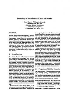
minimizes the OP. Section VI presents the numerical results, while Section VII concludes the paper. II. S YSTEM M ODEL As a starting point, consider a mobile wireless network in which TXs are randomly placed on an infinite 2-D plane according to a homogeneous PPP with spatial density 𝜆𝑠 [nodes/m2 ] and moving independently of each other. At each TX, a series of packets, each with a fixed duration 𝑇 , arrives according to an independent homogeneous 1-D PPP in time with intensity 𝜆𝑡 [packets/sec/node]. These packets are then sent with a constant power 𝜌 to the intended RX, which is assumed to lie a fixed distance 𝑅 away. Futhermore, each packet is given 𝑀 backoffs and 𝑁 retransmission attempts. In this network model, the spatial PPP is first fixed and each TX generates its own traffic of packets. This means that at each time instant, the average number of new packets that are active per unit area is 𝜆 = 𝜆𝑠 𝜆𝑡 𝑇 [packets/m2 ]. Due to the ability to backoff from transmissions (in CSMA) and retransmit in the case of erroneous packet reception, we have an increase of 𝜆Δ(𝑀, 𝑁 ) to the spatial density. Hence, the density of packets attempting to access the channel at each time instant is 𝜆(1 + Δ(𝑀, 𝑁 )). If no backoffs or retransmissions are allowed, i.e., (𝑀, 𝑁 ) = (1, 0), we have that Δ(𝑀, 𝑁 ) = 0 for all the protocols. Note that the number of backoffs 𝑀 is always strictly greater than 0. Since this network model entails two independent Poisson distributions, in order to derive the OP, we would have to average over both the spatial and temporal statistics. Due to the complicated analysis this would entail, instead we consider our wireless network from an alternative point of view; Consider a single queue of packet arrivals with density 𝜆𝑠 𝜆𝑡 𝐴, where 𝐴 is the area of the communication region. Upon the arrival of each packet, it is assigned to a TX node, which is then randomly placed on a 2-D plane (uniformly distributed in area 𝐴), as illustrated in Fig. 1. The transmission to the intended RX is then initiated according to the specified MAC protocol. When the packet has been served (successfully or not), the corresponding TX-RX pair disappears from the plane. When the maximum number of backoffs and retransmissions is not reached, the packet is placed back in the packet arrival queue, with a new transmission time. The retransmitted packet will be located in a new position, which is justified by our assumption on high mobility. Considering the increase in the density of packets attempting to access the channel, we have that 𝜆 = 𝜆𝑠 𝜆𝑡 𝑇 (1 + Δ(𝑀, 𝑁 )). Note that the temporal PPP of packet arrivals at each node is independent of the PPP of TX locations in space. Due to the high mobilility presumed in our network, different sets of packets are active between times 𝑡0 and 𝑡0 + 𝑇 . Since the waiting time from one transmission attempt to the next is set to be greater than 𝑇 , we have that there are no spatial and temporal correlations between retransmission attempts. This is in accordance with the results of [17]. As a result of this independence, and the basic properties of PPPs, we have that the number of nodes in any random selection of an area at any random point in time still follows a PPP [18]. Hence, we have that our space-time model entails a 3-D PPP with density 𝜆𝑠 𝜆𝑡 (1+Δ(𝑀, 𝑁 )) [packets/m2 /sec]. Considering the

242


Fig. 1. Each new packet arrival is assigned to a TX-RX pair, which is then located randomly on a 2-D plane.

entire plane at a fixed point in time, we observe the behaviour of the space-time model’s spatial 2-D PPP with density 𝜆 = 𝜆𝑠 𝜆𝑡 𝑇 (1+Δ(𝑀, 𝑁 )). Equivalently, the total expected number of packets in area 𝐴 during a time interval 𝑇 is 𝜆𝑠 𝜆𝑡 𝐴 𝑇 (1 + Δ(𝑀, 𝑁 )). Thus, we see that our alternative 3-D space-time model is a good representation of the ad hoc network initially described, as it entails a Poisson distribution of nodes in space and of packet arrivals in time, with the same density of packets accessing the channel as the initial model. Hence, we adopt this model for our analysis, as it allows us to only consider a single random process describing both the temporal and spatial variations of the system. Note the following main attributes of our traffic model that are of significance in our derivations: ∙

∙

∙

Our network is highly mobile, meaning that different and independent sets of nodes are observed on the plane from one slot (of length 𝑇 ) to the next. Upon retransmission of a packet, it is treated as a new packet arrival and placed in a new location, resulting in no spatial correlation between transmission attempts. The waiting time between retransmission attempts is set to be 𝑡𝑤𝑎𝑖𝑡 > 𝑇 , which because of the high mobility assumption, results in no temporal correlation between retransmission attempts.

For the channel model, we consider only path loss attenuation effects (with path loss exponent 𝛼 > 2), ignoring both short term and long term fading. The channel is assumed to be constant for the duration of a transmission. Each RX sees interference from all active TXs on the plane, and these interference powers are added to the channel noise, 𝜂, to result in a certain SINR at each RX. If this received SINR falls below the required SINR threshold, 𝛽𝑟𝑒𝑞 , at any time during the packet transmission, the packet is received erroneously and must be retransmitted, with probability ( ) 𝜌𝑅−𝛼 (1) ∑ 𝑃𝑟𝑡 = Pr min −𝛼 ≤ 𝛽𝑟𝑒𝑞 , 0≤𝑡≤𝑇 𝜂 + 𝑖(𝑡) 𝜌𝑟𝑖 where 𝑟𝑖 is the distance between the node under observation and the 𝑖-th interfering TX, and the summation is over all active interferers on the plane at time 𝑡. The MAC protocols ALOHA and CSMA are applied

for communication between nodes. In the case of unslotted ALOHA, each transmission starts as soon as the packet arrives, regardless of the channel condition. Slotted ALOHA improves the performance by removing partial outages, but this requires synchronization. If the packet is received erroneously, it is retransmitted. Each packet has a maximum of 𝑁 retransmission attempts in order to be received correctly. In the CSMA protocol, the channel is sensed at the beginning of each packet. If the measured SINR is above 𝛽𝑠𝑒𝑛𝑠 , the packet transmission is initiated; otherwise, it is backed off. Each packet is given a maximum of 𝑀 backoffs, before it is dropped. Since evaluating the backoff scheme is outside the scope of this work, we simply assume that the backoff times are random, uncorrelated, and exponentially distributed (this also maintains the Poisson distribution of packets). Once the transmission is initiated, but the packet is received erroneously after 𝑁 retransmissions, it is counted to be in outage. Finally, all communication between the TX and its RX is assumed to occur over an orthogonal control channel, and the delay introduced by the feedback is assumed to be insignificant compared to the packet length. In the general sense, the OP of ALOHA and CSMA is defined mathematically as 𝑃𝑜𝑢𝑡 (ALOHA) = ] [ Pr SINR < 𝛽𝑟𝑒𝑞 at some 𝑡 ∈ [0, 𝑇 ) 𝑁 + 1 times , (2) [ 𝑃𝑜𝑢𝑡 (CSMA) = Pr SINR < 𝛽𝑠𝑒𝑛𝑠 at 𝑡 = 0 𝑀 times ∪ ] SINR < 𝛽𝑟𝑒𝑞 at some 𝑡 ∈ (0, 𝑇 ) 𝑁 + 1 times . (3) The throughput 𝑆 of this network is given as: 𝑆 = 𝜆(1 + Δ(𝑀, 𝑁 )) 𝑏 (1 − 𝑃𝑜𝑢𝑡 ) [bits/s/Hz/m2 ], where 𝑏 is the average rate that a successful packet achieves, with units [bits/s/Hz per packet]. Since the OP is the only unknown term in the throughput expression, we will solely focus on this metric in the remainder of this paper.

A. Justification of Assumptions For ad hoc networks with single-hop communication links and substantial mobility or indiscriminate node placement, such as a dense sensor network, an assumption of Poisson distributed nodes in space is reasonable and commonly used [2], [3], [4]. However, in many networks, such as clustered or multi-hop networks, this assumption might not be valid anymore, as transmissions are often correlated with each other in both time and space. Assuming no fading is not always reasonable. This assumption is made because we wish to find the OP of MAC protocols under optimal conditions, as in [4], [5]. In [19], we add fading to our model, and derive the OP of the various protocols. Fading is shown to deteriorate the average performance of the network. The assumption of fixed packet length 𝑇 is reasonable, because in most applications, data to be transmitted is packetized before transmission, and each packet is then of the same constant length. The fixed distance, 𝑅, between all TXRX pairs (which is also assumed in [2], [5], [7]) is often not a natural assumption. However, we know that for low


243

on high mobility, and by selecting the time interval from one retransmission attempt to the next (due to a backoff or retransmission) to be 𝑡𝑤𝑎𝑖𝑡 > 𝑇 , there is no spatial and temporal correlation between the retransmission attempts. Given the probability of a packet being retransmitted in ALOHA is 𝑃𝑟𝑡 , the density of packets on the plane at each time instant is 𝑁 +1 1 − 𝑃𝑟𝑡 . 1 − 𝑃𝑟𝑡 (5) Applying the concept of guard zones in our ad hoc network with spatial node density of 𝜆𝑎𝑙𝑜ℎ𝑎 (𝑃𝑟𝑡 ), we shall now derive the OP of slotted and unslotted ALOHA in the following. 2 𝑁 + ... + 𝑃𝑟𝑡 )=𝜆 𝜆𝑎𝑙𝑜ℎ𝑎 (𝑃𝑟𝑡 ) = 𝜆 (1 + 𝑃𝑟𝑡 + 𝑃𝑟𝑡

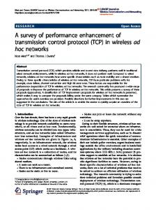
Fig. 2. When at least one interferer TX1 falls within a distance 𝑠 away from RX0 , i.e., inside 𝐵(RX0 , 𝑠), it causes outage for RX0 .

A. Slotted ALOHA densities, the OP is a convex1 function of 𝑅, making our OP analysis yield a lower bound to the case when 𝑅 is variable. Furthermore, it has been rigorously shown in [20] that variable transmit distances do not result in fundamentally different performances. Finally, note that the whole network with a fixed 𝑅 could be viewed as a snapshot of a multi-hop wireless network, where 𝑅 is the bounded average inter-relay distance resulting from the specific routing protocol used. III. O UTAGE P ROBABILITY OF ALOHA The ALOHA protocol is one of the simplest MAC algorithms for a communication network. Here, packets are transmitted to their intended RXs immediately upon their arrival, regardless of the channel conditions. In order to analyze the OP of ALOHA, we apply the concept of guard zones [4]. First, define 𝑠 to be the distance between a randomly selected RX on the plane, RX0 , and its closest interfering TX that causes the SINR to fall just below the threshold 𝛽. By manipulation of the SINR expression, 𝑠 is derived to be: ( −𝛼 )− 𝛼1 𝑅 𝜂 − 𝑠 = . (4) 𝛽 𝜌 Through Eq. (4), 𝛽𝑠𝑒𝑛𝑠 corresponds to 𝑠𝑠𝑒𝑛𝑠 , 𝛽𝑟𝑒𝑞 to 𝑠𝑟𝑒𝑞 , etc. The guard zone 𝐵(RX0 , 𝑠) is a circle of radius 𝑠 around RX0 , as illustrated in Fig. 2. One situation that would cause RX0 to go into outage is if the accumulation of powers from all the interfering nodes outside 𝐵(RX0 , 𝑠) results in the SINR at RX0 falling below the threshold 𝛽. Another situation is if at least one active TX, other than RX0 ’s own TX, TX0 , falls inside 𝐵(RX0 , 𝑠) at any time during the packet transmission. Considering only the latter event yields a lower bound to the OP. It has previously been shown that this lower bound is in fact fairly tight around the actual OP [5], and hence, we only focus on this bound in our analysis. Allowing for retransmissions is equivalent to increasing the average number of packets that attempt to access the channel, when the network is in a steady state. With the assumption 1 Convexity

may be proven by considering the second derivative of 𝑃𝑜𝑢𝑡 . 𝑃𝑜𝑢𝑡 consists of a combination of error probability expressions of the form 2 2 𝑃𝑟𝑡 𝑃𝑟𝑡 = 1 − 𝑒−𝑘𝑅 , where 𝑘 is a function of 𝜆 and 𝛽. Moreover, 𝑑𝑑𝑅 2 = 2

2𝑘𝑒−𝑘𝑅 (1 − 2𝑘𝑅2 ). This is > 0, and thus 𝑃𝑟𝑡 is convex, for 2𝑘𝑅2 < 1, which is the case for low enough densities.

In slotted ALOHA, the time line is divided into slots of fixed duration 𝑇 , and TXs can only start their transmissions at the beginning of the next time slot after each packet has been formed. Thus there is no partial overlap of packets, something that is intuitively expected to decrease the OP compared to unslotted algorithms. This performance improvement comes, however, at the expense of a need for synchronization. Since the system is slotted, we are only concerned with the locations of packet arrivals in each slot, which follow a homogeneous 2-D PPP with intensity 𝜆𝑎𝑙𝑜ℎ𝑎 (𝑃𝑟𝑡,𝑠 ), where 𝑃𝑟𝑡,𝑠 is the probability that a transmission attempt is unsuccessful. By properties of the PPP, the interferers of the node under observation also follow a homogeneous 2-D PPP with the same intensity. This yields the following theorem. Theorem 1: The OP of slotted ALOHA can be lower 𝑁 +1 𝑙𝑏 (Slotted ALOHA) = 𝑃˜𝑟𝑡,𝑠 , where 𝑃˜𝑟𝑡,𝑠 bounded by 𝑃𝑜𝑢𝑡 is the solution to ˜ 𝑁 +1 1−𝑃 𝑟𝑡,𝑠

−𝜆 𝑃˜𝑟𝑡,𝑠 = 1 − 𝑒 1−𝑃˜𝑟𝑡,𝑠

𝜋𝑠2𝑟𝑒𝑞

.

(6)

Proof: Consider the active communication link TX0 -RX0 . Due to the slotting of time, only packets arriving during the last 𝑇 seconds start simultaneously with the one generated by TX0 , and have thus the potential to result in an erroneous packet reception at RX0 . Based on the concept of guard zones, we have that 𝔼 [# of interf. inside 𝐵(RX0 , 𝑠𝑟𝑒𝑞 ) at some 𝑡 ∈ [−𝑇, 0)] ≈ 𝜆𝑎𝑙𝑜ℎ𝑎 (𝑃˜𝑟𝑡,𝑠 ) 𝜋 𝑠2𝑟𝑒𝑞 , (7) where 𝜆𝑎𝑙𝑜ℎ𝑎 (𝑃˜𝑟𝑡,𝑠 ) is given by Eq. (5). The probability of having an erroneous packet transmission in a Poisson distributed network is 𝑃𝑟𝑡,𝑠 = 1−𝑒−𝔼[# of interferers] . Furthermore, a packet is retransmitted the 𝑘-th time if it is erroneously received all 𝑘−1 previous attempts. Hence, a packet is counted to be in outage if it is received erroneously on the 𝑁 -th 𝑙𝑏 (Slotted ALOHA) = retransmission attempt, resulting in 𝑃𝑜𝑢𝑡 𝑁 +1 ˜ 𝑃𝑟𝑡,𝑠 . B. Unslotted ALOHA In unslotted ALOHA, communication is continuous in time, i.e., packets are transmitted as soon as they are formed. Unslotted protocols are particularly of interest in systems that have no synchronization abilities. Intuitively, we expect the OP

244


of unslotted ALOHA to exceed that of the slotted case, due to the partial overlap of transmissions. With the same reasoning as for slotted ALOHA, we obtain the following theorem. Theorem 2: The OP of unslotted ALOHA can be lower 𝑁 +1 𝑙𝑏 (Unslotted ALOHA) = 𝑃˜𝑟𝑡,𝑢 , where 𝑃˜𝑟𝑡,𝑢 bounded by 𝑃𝑜𝑢𝑡 is the solution to ˜ 𝑁 +1 1−𝑃 𝑟𝑡,𝑢

−2𝜆 1−𝑃˜ 𝑟𝑡,𝑢 𝑃˜𝑟𝑡,𝑢 = 1 − 𝑒

𝜋𝑠2𝑟𝑒𝑞

.

(8)

Proof: Due to the unslottedness of the system, any transmission that started less than time 𝑇 before the start of TX0 ’s transmission and up to time 𝑇 later, will be interfering with the packet of RX0 and thus contribute to its OP. Since the number of packet arrivals at times 𝑡0 and 𝑡0 + 𝑇 are independent, we have that ( ) 𝑃˜𝑟𝑡,𝑢 = 1 − Pr No TXs in 𝐵(RX0 , 𝑠𝑟𝑒𝑞 ) during [−𝑇, 𝑇 ) ˜

2

= 1 − 𝑒−2𝜆𝑎𝑙𝑜ℎ𝑎 (𝑃𝑟𝑡,𝑢 ) 𝜋𝑠𝑟𝑒𝑞 , where 𝑃˜𝑟𝑡,𝑢 is the approximate probability of an erroneous packet reception in unslotted ALOHA, with 𝜆𝑎𝑙𝑜ℎ𝑎 (𝑃˜𝑟𝑡,𝑢 ) as given by Eq. (5). Given 𝑁 retransmissions for each packet, the OP becomes 𝑃˜ 𝑁 +1 . 𝑟𝑡,𝑢

For low densities, 𝑃𝑟𝑡,𝑠 ≈ 𝑃𝑟𝑡,𝑢 , allowing us to compare slotted and unslotted ALOHA. Applying the Taylor expansion, we obtain that slotted ALOHA outperforms its unslotted version by a factor of 2. This is expected and consistent with the results obtained from the conventional model [21]. This result is related to the fact that the space-time volume in slotted ALOHA, 𝑉𝑠 = 𝐴𝑇 , is half of that of unslotted ALOHA, 𝑉𝑢 = 2𝐴𝑇 , as only one slot needs to be considered in the slotted system as opposed to two in the unslotted case. IV. O UTAGE P ROBABILITY OF CSMA Due to the poor performance of unslotted ALOHA, a new MAC protocol, termed Carrier-Sensing Multiple Access (CSMA), was proposed by Kleinrock and Tobagi in [9] more than 30 years ago. By introducing channel sensing and the ability to back off from transmissions, the performance of wireless networks was greatly improved. Moreover, several modifications were proposed in order to overcome the inherent hidden and exposed node problems [9] of CSMA. By allowing some kind of communication between the TX and its RX, throughput improvement was achieved. In the following subsections, we extend the work of [9] to consider point-to-point wireless ad hoc networks, and we evaluate the OP performance of CSMA. As explained in Section II, a packet is backed off if the measured or estimated (depending on whether the RX or TX are sensing) SINR is below the sensing threshold, 𝛽𝑠𝑒𝑛𝑠 , at the beginning of its transmission. Up to a maximum of 𝑀 times, the packet then waits a random time before the channel is sensed again and a new decision is made. Once initiated, but received in error at its RX, the packet is retransmitted. This is repeated 𝑁 times before the packet is dropped. These properties yield the following theorem. Theorem 3: The total OP of CSMA may be expressed as 𝑁 ; 𝑃𝑜𝑢𝑡 (CSMA) = 𝑃𝑏𝑀 + (1 − 𝑃𝑏𝑀 ) 𝑃𝑟𝑡1 𝑃𝑟𝑡

(9)

and the density of packets attempting to access the channel is

[

] 𝑁 1 − 𝑃𝑏𝑀 1 − 𝑃𝑟𝑡 𝑀 + (1−𝑃𝑏 )𝑃𝑟𝑡1 , 𝜆𝑐𝑠𝑚𝑎 (𝑃𝑏 , 𝑃𝑟𝑡1 , 𝑃𝑟𝑡 ) = 𝜆 1 − 𝑃𝑏 1 − 𝑃𝑟𝑡 (10) where 𝑃𝑟𝑡1 is the probability that an activated packet is received erroneously at its first transmission attempt and must be retransmitted, and 𝑃𝑟𝑡 is the probability of error in the retransmission attempts. Expressions for 𝑃𝑏 , 𝑃𝑟𝑡1 , and 𝑃𝑟𝑡 are derived in the following subsections. Proof: The proof of Theorem 3 is given in Appendix A. Due to the backoff property of CSMA, and since packets tagged for retransmission do not perform new channel sensing, we multiply the first term of Eq. (10) by (1 − 𝑃𝑏 ) to find the density of active packets; 𝜆𝑎𝑐𝑡𝑖𝑣𝑒 (𝑃𝑏 , 𝑃𝑟𝑡1 , 𝑃𝑟𝑡 ) ( = 𝜆 1 − 𝑃𝑏𝑀 + (1 − 𝑃𝑏𝑀 )𝑃𝑟𝑡1

𝑁

1 − 𝑃𝑟𝑡 1 − 𝑃𝑟𝑡

)

(11) .

In this section, we assume that the sensing threshold, 𝛽𝑠𝑒𝑛𝑠 , based on which the backoff decision is made, is constant and equal to the required SINR for correct reception of packets, 𝛽𝑟𝑒𝑞 . That is, 𝛽𝑠𝑒𝑛𝑠 = 𝛽𝑟𝑒𝑞 = 𝛽 = 0 dB, which is equivalent to 𝑠𝑠𝑒𝑛𝑠 = 𝑠𝑟𝑒𝑞 = 𝑠 ≈ 𝑅. The value 0 dB is chosen in order for the OP to have little dependence on the path loss exponent 𝛼. A. CSMA with Transmitter Sensing In the conventional CSMA protocol, which is employed in many of today’s network standards, such as IEEE 802.11 and 802.16, the TX is the backoff decision maker. That is, when a new packet arrives, the TX immediately measures aggre) ( the 𝜌𝑅−𝛼 − 𝜂 , gate interference power. If this is greater than 𝛽 it backs off; Otherwise, it starts transmitting. Denoting this protocol by CSMATX , its OP is established by Theorem 4. Theorem 4: The total OP of CSMATX is given by Eq. (9), where: ˜𝑏 is the backoff probability, and is found as the ∙ 𝑃𝑏 ≈ 𝑃 solution to 𝑃˜𝑏 = 1 − 𝑒 ∙

( ) ˜𝑁 1−𝑃 −𝜆 1−𝑃˜𝑏𝑀 +(1−𝑃˜𝑏𝑀 )𝑃˜𝑟𝑡1 1−𝑃˜𝑟𝑡 𝜋𝑠2

,

(12)

𝑇𝑋 𝑃˜𝑏 + (1 − 𝑃˜𝑏)𝑃˜𝑑𝑢𝑟𝑖𝑛𝑔

𝑃𝑟𝑡 ≈ is the probability that an activated packet is received erroneously in a retransmission attempt, with 𝑃˜𝑑𝑢𝑟𝑖𝑛𝑔 being the probability that the error occurs at some 𝑡 ∈ (0, 𝑇 ); − 𝑇𝑋 𝑃˜𝑑𝑢𝑟𝑖𝑛𝑔 = 1−𝑒

∙

𝑟𝑡

∫𝑠

[ ( 2 )] 2 −𝑠2 𝜆𝑐𝑠𝑚𝑎 2𝜋−2 cos−1 𝑟 +𝑅 𝑟 𝑑𝑟 2𝑅𝑟

, (13) with 𝜆𝑐𝑠𝑚𝑎 = 𝜆𝑐𝑠𝑚𝑎 (𝑃𝑏 , 𝑃𝑟𝑡1 , 𝑃𝑟𝑡 ) as given by Eq. (10). 𝑇𝑋 𝑃𝑟𝑡1 ≈ 𝑃˜𝑟𝑥∣𝑡𝑟𝑎𝑛𝑠𝑚𝑖𝑡 + (1 − 𝑃˜𝑟𝑥∣𝑡𝑟𝑎𝑛𝑠𝑚𝑖𝑡 )𝑃˜𝑑𝑢𝑟𝑖𝑛𝑔 is the probability that an activated packet is received erroneously at the first transmission attempt, with 𝑃˜𝑟𝑥∣𝑡𝑟𝑎𝑛𝑠𝑚𝑖𝑡 being the probability that the RX is in outage upon the packet arrival, given its TX decides to 𝑠−𝑅


transmit; 𝑃˜𝑟𝑥∣𝑡𝑟𝑎𝑛𝑠𝑚𝑖𝑡 [ ( √ (𝑅) 1 − 𝑅𝑠 1 − = 𝑃˜𝑏 1 − 2 2𝑠2 cos−1 2𝑠 𝜋𝑠

𝑅2 4𝑠2

(14) )] .

Proof: The proof of Theorem 4 is given in Appendix B. Due to the inter-dependence between 𝑃𝑏 , 𝑃𝑑𝑢𝑟𝑖𝑛𝑔 , and 𝜆𝑐𝑠𝑚𝑎 , their values are found through numerical iterations. Also, the reason Eqs. (12)-(14) are approximations is that the concept of guard zones is used to derive a lower bound, while the assumption that all new interferers ignore each other and make their backoff decision based on TX0 only, increases the OP above the lower bound. This is discussed further in Appendix B. The OP of CSMATX is due to the hidden and exposed node problems. The hidden node problem occurs when a new interferer TX𝑖 is located inside 𝐵(RX0 , 𝑠) ∩ 𝐵(TX0 , 𝑠), where TX0 is hidden to TX𝑖 , during all the 𝑁 retransmission attempts of the packet of TX0 -RX0 . However, compared to unslotted ALOHA, CSMATX improves the OP by avoiding transmissions inside 𝐵(TX0 , 𝑠) ∩ 𝐵(RX √ 0 ,(𝑠). )The area of this ( ) 𝑅 2 2 −1 𝑅 region is 𝐴 = 2𝑠 cos 2𝑠 − 𝑅𝑠 1 − 2𝑠 . The exposed node problem occurs when TX𝑖 backs off in cases when its transmission would not have contributed to any outage, i.e., when TX𝑖 is located inside 𝐵(TX0 , 𝑠) ∩ 𝐵(RX0 , 𝑠) during all the 𝑀 backoffs. This adds to the OP of unslotted ALOHA. Hence, we have that (15) 𝑃𝑜𝑢𝑡 (CSMATX ) ≈ 𝑃𝑜𝑢𝑡 (Unslotted ALOHA) )𝑀 ( ( ) 2 𝑁 − 1 − 𝑒−𝜆𝑎𝑐𝑡𝑖𝑣𝑒 𝐴 + 1 − 𝑒−𝜆𝑎𝑐𝑡𝑖𝑣𝑒 (𝜋𝑠 −𝐴) , where 𝜆𝑎𝑐𝑡𝑖𝑣𝑒 is given by Eq. (11). This approximation works best for low densities, i.e., when 𝜆𝑎𝑐𝑡𝑖𝑣𝑒 ≈ 𝜆𝑎𝑙𝑜ℎ𝑎 . To better understand the behavior of the backoff probability, let w.l.o.g. (𝑀, 𝑁 ) = (1, 0). 𝑃𝑏 can then be expressed in terms of the Lambert function, 𝑊0 (⋅) [1]. Let 𝑥 = 𝜆𝜋𝑠2 in Eq. (12), and apply l’Hopital’s rule: lim

𝑥→0

1

− 𝑥1 𝑊0 (𝑥) 1 − 𝑒−𝑥

= lim

𝑥→0

𝑥 − 𝑊0 (𝑥) 𝑥(1 − 𝑒−𝑥 )

0 (𝑥) 1 − 𝑑𝑊𝑑𝑥 𝑥→0 1 − 𝑒−𝑥 + 𝑥𝑒−𝑥 𝑒𝑊0 (𝑥) + 𝑥 − 1 = lim 𝑊 (𝑥) 𝑥→0 (𝑒 0 + 𝑥) [𝑒−𝑥 (𝑥 − 1) + 1] 1 = lim 𝑒𝑊0 (𝑥) +𝑥 𝑥→0 [𝑒−𝑥 (𝑥−1)+1] + 𝑊0 (𝑥) 𝑑𝑊0 (𝑥)

= lim

= 1.

𝑒

𝑑𝑥

+1

[−𝑒−𝑥 (𝑥−1)+𝑒−𝑥 ]

This proves that as 𝜆 → 0, 𝑃𝑏 → 𝑃𝑜𝑢𝑡 (Slotted ALOHA). Equivalently, for a fixed backoff probability 𝑃 𝑏 , we have that the density of active packets in CSMA is 𝜆𝑎𝑐𝑡𝑖𝑣𝑒 = 𝜆𝑎𝑙𝑜ℎ𝑎 (𝑃˜𝑟𝑡,𝑠 ) . For low 𝑃𝑏 , 𝜆𝑎𝑐𝑡𝑖𝑣𝑒 ≈ 𝜆𝑎𝑙𝑜ℎ𝑎 , while as 𝑃𝑏 1−𝑃 𝑏 increases, the density of active transmissions in CSMA may no longer be approximated by that of ALOHA. Due to the reduced number of interferers, 𝑃𝑏 is less than the case when all prior arrivals are activated. Hence, while Eq. (12) is an

245

approximate measure of 𝑃𝑏 , Eq. (6) operates as an upper bound. B. CSMA with Receiver Sensing With the objective of improving the performance of CSMA, we introduce a novel protocol, termed CSMARX . In this protocol, the RX senses the channel and subsequently determines whether or not the packet transmission should be initiated. The communication between the TX and RX is assumed to occur over a separate 1 bit control channel, and the delay introduced by the feedback is assumed to be small and insignificant compared to the packet length. The OP of CSMARX is given by the following theorem. Theorem 5: The total OP of CSMARX is given by Eq. (9), where: ˜𝑏 is the backoff probability, found as the solution ∙ 𝑃𝑏 ≈ 𝑃 𝑅𝑋 to Eq. (12); 𝑃𝑟𝑡1 ≈ 𝑃˜𝑑𝑢𝑟𝑖𝑛𝑔 , given below; 𝑅𝑋 ˜ ˜ ˜ ∙ 𝑃𝑟𝑡 ≈ 𝑃𝑏 + (1 − 𝑃𝑏 )𝑃𝑑𝑢𝑟𝑖𝑛𝑔 is the probability that an activated packet is received erroneously some time during its transmission and must thus be retransmitted; ( ) 𝑅𝑋 𝑃˜𝑑𝑢𝑟𝑖𝑛𝑔 = 1−𝑒

−

∫𝑠

𝑠−𝑅

∫ 2𝜋−𝜈(𝑟) 𝜈(𝑟)

𝜆𝑐𝑠𝑚𝑎 𝑃 (active∣𝑟,𝜙)𝑟 𝑑𝜙 𝑑𝑟

, (16) where 𝜆𝑐𝑠𝑚𝑎 = 𝜆𝑐𝑠𝑚𝑎 (𝑃𝑏 , 𝑃𝑟𝑡1 , 𝑃𝑟𝑡 ) is given by Eq. (10), and 𝑃 (active∣𝑟, 𝜙) and 𝜈(𝑟) are: ( ) 2 2 2 1 √ 2 −𝑠2 −2𝑅𝑟 cos 𝜙 , 𝑃 (active∣𝑟, 𝜙) = 1 − cos−1 𝑟 +2𝑅 2𝑅 𝑟 +𝑅 −2𝑅𝑟 cos 𝜙 𝜋 ( 2 ) 2 𝑟 + 2𝑅𝑠 − 𝑠 𝜈(𝑟) = cos−1 . (17) 2𝑅𝑟 Proof: The proof of Theorem 5 is given in Appendix C. The OP of CSMARX is due to the hidden node problem, which occurs when an interferer is located inside 𝐵(RX0 , 𝑠), while its RX is located in 𝐵(TX0 , 𝑠). This is discussed further in Sections V-B and VI. V. O PTIMIZING THE S ENSING T HRESHOLD Our objective in this section is to optimize the sensing threshold, 𝛽𝑠𝑒𝑛𝑠 , of CSMA in its various incarnations, in order to minimize the OP. In the analysis thus far, we have used a constant sensing threshold, namely 𝛽𝑠𝑒𝑛𝑠 = 𝛽𝑟𝑒𝑞 = 𝛽 = 0 dB. In this section, we take into account variations in 𝛽𝑠𝑒𝑛𝑠 (translating to 𝑠𝑠𝑒𝑛𝑠 by Eq. (4)). For the sake of readability of the formulas, we denote 𝑠𝑠𝑒𝑛𝑠 by 𝑠. Initially, we assume that 𝛽𝑟𝑒𝑞 stays constant (w.l.o.g., we assume that 𝛽𝑟𝑒𝑞 = 0 dB, which corresponds to 𝑠𝑟𝑒𝑞 ≈ 𝑅), while 𝛽𝑠𝑒𝑛𝑠 varies. Next, in Section V-C, we set 𝛽𝑠𝑒𝑛𝑠 = 𝛽𝑟𝑒𝑞 , and allow both the thresholds to vary. We consider both CSMATX and CSMARX , and derive their OPs based on the following subsections. A. CSMA with Transmitter Sensing When 𝑠 varies, it results in changes in the area of 𝐵(TX0 , 𝑠). This impacts 𝑃𝑏 , 𝑃𝑟𝑡1 , and 𝑃𝑟𝑡 , as seen below. Theorem 6: The total OP of CSMATX for varying sensing thresholds is given by Eq. (9), where:

246


𝑇𝑋 𝑃˜𝑑𝑢𝑟𝑖𝑛𝑔

𝑃˜𝑟𝑥∣𝑡𝑟𝑎𝑛𝑠𝑚𝑖𝑡

] [∫ ⎧ ∫ 𝑠𝑟𝑒𝑞 [ 𝑅−𝑠 ( 2 2 2 )]   −𝑠  2𝜋 − 2 cos−1 𝑟 +𝑅 𝑟 𝑑𝑟 −𝜆𝑐𝑠𝑚𝑎 2𝜋 𝑟 𝑑𝑟 +  2𝑅𝑟   0 𝑅−𝑠  ⎨1 − 𝑒 ∫ 𝑠𝑟𝑒𝑞 [ ( 2 2 2 )] = −𝑠  2𝜋 − 2 cos−1 𝑟 +𝑅 𝑟 𝑑𝑟 −𝜆𝑐𝑠𝑚𝑎  2𝑅𝑟   𝑠−𝑅  1 − 𝑒   ⎩ 0

;𝑠 < 𝑅 ; 𝑅 ≤ 𝑠 < 𝑅 + 𝑠𝑟𝑒𝑞 ; otherwise

⎧ ( 2 2 2 ) ( 2 2 2) 𝑠2 1  −1 𝑅 +𝑠 −𝑠𝑟𝑒𝑞 −1 𝑅 +𝑠𝑟𝑒𝑞 −𝑠  𝑃 cos − 𝑃 cos − 𝑃 𝑟𝑥 𝑟𝑥 𝑟𝑥  2𝑅𝑠 2𝑅𝑠𝑟𝑒𝑞  𝜋𝑠2𝑟𝑒𝑞 𝜋 ⎨ √ 𝑃 𝑟𝑥 = + (𝑠 + 𝑠𝑟𝑒𝑞 − 𝑅)(𝑠 − 𝑠𝑟𝑒𝑞 + 𝑅)(−𝑠 + 𝑠𝑟𝑒𝑞 + 𝑅)(𝑠 + 𝑠𝑟𝑒𝑞 + 𝑅) ; 𝑠 < 𝑅 + 𝑠𝑟𝑒𝑞  2  2𝜋𝑠  𝑟𝑒𝑞  ⎩ 0 ; otherwise

𝑅𝑋 𝑃˜𝑑𝑢𝑟𝑖𝑛𝑔 = ] [∫ ∫ ⎧ ∫ 𝜁(𝑟) ∫ ∫ −𝜆𝑐𝑠𝑚𝑎 0𝑠 02𝜋 𝑃 (active∣𝑟,𝜙)𝑟𝑑𝜙𝑑𝑟+2 𝑠𝑠𝑟𝑒𝑞 𝜈(𝑟) 𝑃 (active∣𝑟,𝜙)𝑟 𝑑𝜙𝑑𝑟+ 𝑠𝑠𝑟𝑒𝑞 [2𝜋−2(𝜁(𝑟)−𝜈(𝑟))]𝑟 𝑑𝑟   1−𝑒  ] [∫  ∫ ∫ 𝑠𝑟𝑒𝑞 ∫ 2𝜋−𝜈(𝑟)  2𝑅−𝑠 2𝜋 ⎨ −𝜆 𝑃 (active∣𝑟,𝜙)𝑟 𝑑𝜙 𝑑𝑟+ 2𝑅−𝑠 𝑃 (active∣𝑟,𝜙)𝑟 𝑑𝜙 𝑑𝑟 0 𝜈(𝑟) 1 − 𝑒 𝑐𝑠𝑚𝑎 0 ∫ 𝑠𝑟𝑒𝑞 ∫ 2𝜋−𝜈(𝑟)  𝑃 (active∣𝑟,𝜙)𝑟 𝑑𝜙 𝑑𝑟 1 − 𝑒−𝜆𝑐𝑠𝑚𝑎 𝑠−2𝑅 𝜈(𝑟)    ⎩ 0

∙

∙

∙

(18)

𝑃𝑏 ≈ 𝑃˜𝑏 is given by Eq. (12); and 𝑃˜𝑟𝑥 = 1 − 2 𝑒−𝜋𝜆𝑎𝑐𝑡𝑖𝑣𝑒 𝑠𝑟𝑒𝑞 is the approximate probability that the RX is in outage upon arrival in each retransmission attempt with 𝜆𝑎𝑐𝑡𝑖𝑣𝑒 given by Eq. (11). 𝑇𝑋 𝑃𝑟𝑡 ≈ 𝑃˜𝑟𝑥 + (1 − 𝑃˜𝑟𝑥 )𝑃˜𝑑𝑢𝑟𝑖𝑛𝑔 is the probability that an activated packet is received erroneously in a retransmission attempt, with 𝑃˜𝑑𝑢𝑟𝑖𝑛𝑔 being the probability that the error occurs at some 𝑡 ∈ (0, 𝑇 ). This is given by Eq. (18). 𝑇𝑋 𝑃𝑟𝑡1 ≈ 𝑃˜𝑟𝑥∣𝑡𝑟𝑎𝑛𝑠𝑚𝑖𝑡 + (1 − 𝑃˜𝑟𝑥∣𝑡𝑟𝑎𝑛𝑠𝑚𝑖𝑡 )𝑃˜𝑑𝑢𝑟𝑖𝑛𝑔 is probability that the first transmission is erroneous, with 𝑃˜𝑟𝑥∣𝑡𝑟𝑎𝑛𝑠𝑚𝑖𝑡 being the probability that the RX is in outage at the start of the packet. This is given by Eq. (19).

∙

∙

(19)

(20) ;0 < 𝑠 < 𝑅 ; 𝑅 ≤ 𝑠 < 2𝑅 ; 2𝑅 ≤ 𝑠 < 2𝑅 + 𝑠𝑟𝑒𝑞 ; otherwise

𝑇𝑋 𝑃𝑟𝑡 ≈ 𝑃˜𝑟𝑥 + (1 − 𝑃˜𝑟𝑥 )𝑃˜𝑑𝑢𝑟𝑖𝑛𝑔 is the probability that an activated packet is received erroneously in a retransmission attempt, with 𝑃˜𝑑𝑢𝑟𝑖𝑛𝑔 being the probability that the error occurs at some 𝑡 ∈ (0, 𝑇 ). This is given by Eq. (20), where 𝑃 (active∣𝑟, ( 2 𝜙) and2 𝜈(𝑟) ) are given by Eq. (17), and . 𝜁(𝑟) = cos−1 𝑟 −2𝑅𝑠−𝑠 2𝑅𝑟 𝑅𝑋 𝑃𝑟𝑡1 ≈ 𝑃˜𝑟𝑥∣𝑡𝑟𝑎𝑛𝑠𝑚𝑖𝑡 + (1 − 𝑃˜𝑟𝑥∣𝑡𝑟𝑎𝑛𝑠𝑚𝑖𝑡 )𝑃˜𝑑𝑢𝑟𝑖𝑛𝑔 is the probability that the first transmission attempt is erroneous, with 𝑃˜𝑟𝑥∣𝑡𝑟𝑎𝑛𝑠𝑚𝑖𝑡 being the probability that the RX is in outage at the start of the packet; [ ] { 2 ; 𝑠 < 𝑠𝑟𝑒𝑞 𝑃𝑟𝑥 1 − 𝑠𝑠2 ˜ 𝑟𝑒𝑞 (21) 𝑃𝑟𝑥∣𝑡𝑟𝑎𝑛𝑠𝑚𝑖𝑡 = 0 ; otherwise

Proof: The proof of Theorem 6 is given in Appendix D.

Proof: The proof of Theorem 7 is given in Appendix E.

Optimizing the sensing threshold in CSMATX yields an optimal tradeoff between the hidden and exposed node problems, as also mentioned in Section IV-A. An increase in one problem (by changing 𝑠) leads to a decrease in the other, and vice versa. This is discussed further in Section VI.

Our simulation results indicate that the optimal sensing threshold in CSMARX is 𝛽𝑠𝑒𝑛𝑠 = 𝛽𝑟𝑒𝑞 (equivalent to 𝑠𝑠𝑒𝑛𝑠 = 𝑠𝑟𝑒𝑞 ). To understand this, consider w.l.o.g. the case of (𝑀, 𝑁 ) = (1, 0), simplifying Eq. (9) to 𝑃˜𝑡𝑜𝑡𝑎𝑙

=

B. CSMA with Receiver Sensing In this section, we wish to improve the performance of CSMARX by optimizing the sensing threshold. Following a similar analysis as in Section IV-B, we establish the following theorem. Theorem 7: The total OP of CSMARX for varying sensing thresholds is given by Eq. (9), where: ˜𝑏 is given by Eq. (12); 𝑃˜𝑟𝑥 is given in Theorem ∙ 𝑃𝑏 ≈ 𝑃 6; and

=

𝑃˜𝑜𝑢𝑡 (CSMARX ) { 𝑅𝑋 𝑃˜𝑟𝑥 + (1 − 𝑃˜𝑟𝑥 ) 𝑃˜𝑑𝑢𝑟𝑖𝑛𝑔 𝑃˜𝑏 + (1 − 𝑃˜𝑏 ) 𝑃˜ 𝑅𝑋 𝑑𝑢𝑟𝑖𝑛𝑔

(22) ; 𝑠 < 𝑠𝑟𝑒𝑞 ; otherwise

Based on this, we now evaluate the rate of change of the 𝑅𝑋 different sources of outage, namely 𝑃˜𝑏 and 𝑃˜𝑑𝑢𝑟𝑖𝑛𝑔 . ∙

When 𝑠 < 𝑠𝑟𝑒𝑞 : 𝑅𝑋 𝑑𝑃˜𝑑𝑢𝑟𝑖𝑛𝑔 𝑑𝑃˜𝑡𝑜𝑡𝑎𝑙 = [1 − 𝑃˜𝑟𝑥 ] . 𝑑𝑠 𝑑𝑠

(23)

Since 𝑃˜𝑟𝑥 is only a function of 𝑠𝑟𝑒𝑞 , its derivative


247

𝑠 ≥ 𝑠𝑟𝑒𝑞 . Thus, we conclude that the OP of CSMARX is minimized 𝑜𝑝𝑡 for 𝛽𝑠𝑒𝑛𝑠 = 𝛽𝑟𝑒𝑞 (i.e., 𝑠𝑜𝑝𝑡 𝑠𝑒𝑛𝑠 = 𝑠𝑟𝑒𝑞 ). Note that the reduction 𝑜𝑝𝑡 is more evident at higher densities, in the OP by using 𝛽𝑠𝑒𝑛𝑠 as will be discussed in Section VI. C. Dependence of OP on the Required SINR Threshold

Fig. 3. The setup used in Section V-B to illustrate the rate of increase in 𝑃𝑏 and decrease in 𝑃𝑑𝑢𝑟𝑖𝑛𝑔 as 𝛽 increases.

∙

𝑅𝑋 with respect to 𝑠 is 0. 𝑃˜𝑑𝑢𝑟𝑖𝑛𝑔 on the other hand is a monotonically decreasing function of 𝑠, which can be observed by considering Fig. 3. As 𝑠 increases with 𝑑𝑠, the areas A and C shrink. As the decrease in these 𝑅𝑋 than the increase areas has a greater impact on 𝑃˜𝑑𝑢𝑟𝑖𝑛𝑔 in area B (because in A and C, 𝑃 (active∣𝑟, 𝜙) = 1), 𝑅𝑋 we get a decrease in 𝑃˜𝑑𝑢𝑟𝑖𝑛𝑔 . Intuitively, this means that an increase in 𝑠 results in more protection for an arriving TX-RX pair, resulting in a higher rate of backoff. Consequently, due to the reduced number of interferers, there is a smaller probability that a packet transmission goes into outage once it has been activated. Hence, 𝑑𝑃˜𝑡𝑜𝑡𝑎𝑙 < 0 for 𝑠 < 𝑠𝑟𝑒𝑞 . 𝑑𝑠 When 𝑠 ≥ 𝑠𝑟𝑒𝑞 :

] 𝑑𝑃˜ ] 𝑑𝑃˜ 𝑅𝑋 [ [ 𝑑𝑃˜𝑡𝑜𝑡𝑎𝑙 𝑏 𝑑𝑢𝑟𝑖𝑛𝑔 𝑅𝑋 = 1 − 𝑃˜𝑑𝑢𝑟𝑖𝑛𝑔 + 1 − 𝑃˜𝑏 . 𝑑𝑠 𝑑𝑠 𝑑𝑠 (24) When 𝑠 increases by 𝑑𝑠, 𝐵(RX0 , 𝑠) grows and so does 𝑃˜𝑏 . The rate of this increase is: 𝑑𝑃˜𝑏 𝜋(𝑠 + 𝑑𝑠)2 − 𝜋𝑠2 𝑑𝑠2 + 2𝑠 𝑑𝑠 ≈ = . (25) 2 𝑑𝑠 𝜋𝑠 𝑠2 𝑅𝑋 𝑃˜𝑑𝑢𝑟𝑖𝑛𝑔 , on the other hand, decreases with 𝑠. This change may be approximated by the decrease in the area around RX0 within which the occurrence of an interferer would cause outage, given by: ( ( 2 2) 2) 𝑅𝑋 𝑑𝑃˜𝑑𝑢𝑟𝑖𝑛𝑔 − 𝜋𝑠2𝑟𝑒𝑞 − 𝜋(𝑠−𝑅) 𝜋𝑠𝑟𝑒𝑞 − 𝜋(𝑠+𝑑𝑠−𝑅) 3 3 ≈ 𝑑𝑠 𝜋𝑠2𝑟𝑒𝑞 2(𝑠 − 𝑅)𝑑𝑠 + 𝑑𝑠2 = − . (26) 3𝑠2𝑟𝑒𝑞 ˜

𝑡𝑜𝑡𝑎𝑙 , we make some approxiTo obtain the sign of 𝑑𝑃𝑑𝑠 mations. Since 𝑑𝑠 ≪ 1, we set (𝑑𝑠)2 ≈ 0. Also, since 𝛽𝑟𝑒𝑞 = 1, and the noise is small, we have 𝑠𝑟𝑒𝑞 ≈ 𝑅. The largest rate of decrease of Eq. (26) is when 𝑠 = 𝑠𝑟𝑒𝑞 + 𝑅.

This yields ∣

𝑅𝑋 𝑑𝑃˜𝑑𝑢𝑟𝑖𝑛𝑔 ∣ 𝑑𝑠

≈

1 3𝑠𝑟𝑒𝑞

0 for

In this section, we assume that both the sensing threshold and the required SINR threshold are varying, while at the same time remaining equal, i.e., 𝛽𝑠𝑒𝑛𝑠 = 𝛽𝑟𝑒𝑞 = 𝛽 (equivalently 𝑠𝑠𝑒𝑛𝑠 = 𝑠𝑟𝑒𝑞 = 𝑠). The total OP of CSMATX is then found by replacing 𝑠𝑟𝑒𝑞 by 𝑠 in Theorem 6, with the following differences: ∙ The approximate probability that the RX is in outage at the start of its first transmission attempt, is: 𝑃˜𝑟𝑥∣𝑡𝑟𝑎𝑛𝑠𝑚𝑖𝑡 = ⎧ ⎨𝑃𝑟𝑥 [ ⎩𝑃𝑟𝑥 1 −

2 𝜋

(𝑅) + cos−1 2𝑠

(27) 𝑅 2

] ;𝑠 < √ ) ( 2 𝑅 𝑅 1 − 2𝑠 ; otherwise 𝜋𝑠

The approximate probability that a packet goes into outage at some 𝑡 ∈ (0, 𝑇 ) is now given by Eq. (28). The OP of CSMARX is found by setting 𝑠𝑟𝑒𝑞 = 𝑠𝑠𝑒𝑛𝑠 = 𝑠 in Theorem 7, with the difference that the third line in Eq. (20) is now valid for all 𝑠 ≥ 2𝑅. ∙

VI. N UMERICAL R ESULTS For the simulations, we generate, as described in Section II, the 3-D PPP of packets over an area of 𝐴 = 1000 m2 , and set w.l.o.g. 𝑅 and 𝜌 to be 1, and the path loss exponent 𝛼 = 4. The derived formulas for slotted and unslotted ALOHA are plotted in Fig. 4 for (𝑀, 𝑁 ) = (1, 0),2 and seen to follow the simulation results tightly for all densities. The curves confirm Theorems 1 and 2, and that the slotted system outperforms the unslotted one by approximately a factor of 2. Moreover, we observe that the OP of ALOHA increases linearly with the number of active interferers on the plane (which is equal to the number of packet arrivals), until it reaches a saturation point where OP ≈ 1. For the sake of the discussions in Section IV-A, the backoff probability of CSMA, 𝑃𝑏 , is also plotted in Fig. 4. For low densities, 𝑃𝑏 is approximately equal to the OP of slotted ALOHA. For higher densities, due to fewer active interferers in CSMA, 𝑃𝑏 < 𝑃𝑜𝑢𝑡 (Slotted ALOHA). Fig. 5 shows the OP performance of CSMATX and CSMARX for (𝑀, 𝑁 ) = (1, 0) and (𝑀, 𝑁 ) = (2, 1). The analytical expressions are confirmed as they are seen to follow the simulations tightly for (𝑀, 𝑁 ) = (1, 0). However, for (𝑀, 𝑁 ) = (2, 1), we observe a greater discrepancy. This is due to the fact that the guard zone approximation is used multiple times when 𝑀 > 1 and 𝑁 > 0. Clearly, the OP performance of CSMA is considerably reduced by increasing 𝑀 and 𝑁 . In order to compare the different protocols, in Fig. 6, the ratio of the OP of CSMATX and CSMARX over that 2 In [22], the exact OP of slotted ALOHA for 𝛼 = 4 is derived √ to be: 𝑃𝑜𝑢𝑡 (Slotted ALOHA) = 1 − erfc( 𝜋𝛽𝜆𝜋𝑅2 /2). Extending this √ to unslotted ALOHA yields: 𝑃𝑜𝑢𝑡 (Unslotted ALOHA) = 1 − erfc( 𝜋𝛽𝜆𝜋𝑅2 /2)2 . These expressions are also plotted in Fig. 4.

248


𝑇𝑋 𝑃˜𝑑𝑢𝑟𝑖𝑛𝑔

⎧ 2  1 − 𝑒−𝜆𝑐𝑠𝑚𝑎 𝜋 𝑠    ] [  ∫ 𝑠 [ ∫ 𝑅−𝑠  ( 2 2 2 )]   −𝑠 ⎨ 2𝜋 − 2 cos−1 𝑟 +𝑅 𝑟 𝑑𝑟 −𝜆𝑐𝑠𝑚𝑎 2𝜋 𝑟 𝑑𝑟 + 2𝑅𝑟 = 0 𝑅−𝑠 1 − 𝑒    ∫ 𝑠 [ ( 2 2 2 )]    −𝑠  2𝜋 − 2 cos−1 𝑟 +𝑅 𝑟 𝑑𝑟 − 𝜆  𝑐𝑠𝑚𝑎 2𝑅𝑟 ⎩ 𝑠−𝑅 1−𝑒

0

;

𝑅 2

𝑅 8 dB), both CSMA protocols actually perform better than slotted ALOHA. This is because for large 𝑠, 𝐵(TX0 , 𝑠) and 𝐵(RX0 , 𝑠) overlap almost completely, such that the only source of outage in CSMA is if an interferer is placed inside 𝐵(RX0 , 𝑠) during (0, 𝑇 ), as is the case in slotted ALOHA. Moreover, due to the backoff property of CSMA, the density of interferers is lower than that of ALOHA, making CSMA yield a lower OP. Similar behavior is observed for lower densities and other (𝑀, 𝑁 )-values. VII. C ONCLUSION AND F UTURE R ESEARCH In this paper, we have considered the performance of the ALOHA and CSMA MAC protocols in terms of outage probability (OP). Our ad hoc network model represents a communication system in which TX-RX pairs are randomly placed on a 2-D plane, and packets arrive continuously in time based on a 1-D PPP. Within our SINR-based model, we derive expressions for the OP of slotted and unslotted ALOHA, CSMA with TX sensing (CSMATX ) and CSMA with RX sensing (CSMARX ). Our derived analytical expressions are consistent with the simulations, and an intuitive understanding is established on the benefits of CSMA over ALOHA. An interesting result is that when no backoffs or retransmissions are allowed, CSMATX actually performs worse than unslotted ALOHA for low densities due to the exposed node problem. By allowing the RX to sense the channel in CSMARX and inform its TX over a control channel whether or not to initiate its transmission, the performance of the conventional CSMA is significantly improved. Moreover, we optimize CSMA’s sensing threshold, 𝛽𝑠𝑒𝑛𝑠 . We observe that in particular at higher densities, significant performance gain can be obtained by optimizing the sensing 𝑜𝑝𝑡 = 𝛽𝑟𝑒𝑞 . The OP of threshold, which is derived to be 𝛽𝑠𝑒𝑛𝑠 CSMATX and CSMARX can then be reduced by up to 40% and 42% (for (𝑀, 𝑁 ) = (2, 1)), respectively. This optimized sensing threshold is slightly greater than 𝛽𝑟𝑒𝑞 at high densities,

250


due to the extra protection it provides against the aggregate interference from the TXs outside 𝐵(RX0 , 𝑠𝑟𝑒𝑞 ). In other related works, we have investigated the impact of fading on the OP [19], and moreover optimized the OP of ALOHA and CSMA by allowing for bandwidth partitioning [23]. Other possible extensions are to apply adaptive rate and power control to improve the performance of CSMA in wireless ad hoc networks. A PPENDIX A. Proof of Theorem 3 Denote the received SINR of the RX under observation, RX0 , by SINR0 . The packet transmission of TX0 -RX0 is counted to be in outage if one or both of the following events occur: 𝑎) The packet is backed off (i.e., SINR0 < 𝛽 upon packet arrival) 𝑀 times and thus dropped. 𝑏) Once the packet transmission is initiated, one or both of the following subevents occur 𝑁 + 1 times: 𝑏1 ) SINR0 < 𝛽 at the start of the packet, i.e., 𝑡 = 0. 𝑏2 ) SINR0 < 𝛽 at some 𝑡 ∈ (0, 𝑇 ). where events (𝑎) and (𝑏) are independent except at the first transmission attempt. This yields: 𝑃𝑜𝑢𝑡 (CSMA) = Pr(𝑎) + (1 − Pr(𝑎)) Pr(𝑏1 ∪ 𝑏2 ∣𝑎)𝑁 +1 (29) = Pr(𝑎) − (1 − Pr(𝑎)) Pr(𝑏1 ∪ 𝑏2 )𝑁 Pr(𝑏1 ∪ 𝑏2 ∣𝑎), where the probability of events (𝑎) and (𝑏) are derived in the following appendices. Eq. (10) is derived as 𝜆𝑐𝑠𝑚𝑎 (𝑃𝑏 , 𝑃𝑟𝑡1 , 𝑃𝑟𝑡 ) = { ∑𝑀−1 𝑚 𝜆 [ 𝑚=0 𝑃𝑏 ; for 𝑁 = 0 ∑𝑀−1 𝑚 ∑𝑁 −1 𝑛 ] 𝑀 𝜆 ; for 𝑁 ≥ 1 𝑚=0 𝑃𝑏 + (1 − 𝑃𝑏 )𝑃𝑟𝑡1 𝑛=0 𝑃𝑟𝑡 B. Proof of Theorem 4 Based on Eq. (29), the probability that event (𝑎) occurs is Pr(𝑎) ≈ 𝑃𝑏𝑀 , where 𝑃𝑏 can be lower bounded by considering packet arrivals inside 𝐵(TX0 , 𝑠) during [−𝑇, 0). We assume that the number of active interferers on the plane follows a PPP (which is proven by simulation results to be reasonable) with density 𝜆𝑎𝑐𝑡𝑖𝑣𝑒 , as given by Eq. (11). Applying the OP expression for PPPs, 1 − 𝑒−𝔼[# of active interferers] , we reach Eq. (12). Event 𝑏1 is concerned with packet arrivals during [−𝑇, 0), resulting in Pr(𝑏1 ) ≈ 𝑃𝑏 . For the first transmission attempt, Pr(𝑏1 ∣𝑎) is found geometrically as the ratio of the area of 𝐵2 = 𝐵(RX0 , 𝑠) ∩ 𝐵(TX0 , 𝑠) over the area of 𝐵(RX0 , 𝑠), derived to be Eq. (14). For all retransmissions, Pr(𝑏1 ∣𝑎) = 𝑇𝑋 Pr(𝑏1 ) = 𝑃𝑑𝑢𝑟𝑖𝑛𝑔 . Pr(𝑏2 ) is lower bounded by the probability that one or more interfering TXs are located and activated inside 𝐵(RX0 , 𝑠) at some 𝑡 ∈ (0, 𝑇 ). We assume that all interferers (following a PPP with density 𝜆𝑐𝑠𝑚𝑎 ) base their backoff decision on the interference they see only from TX0 . Since 𝜌𝑑−𝛼 𝜌𝑑−𝛼 𝜂 + interf. from TX0 ≥ 𝜂 + interf. from TX0 and all other TXs : Pr [≥ 1 interferer in 𝐵(RX0 , 𝑠) at some 𝑡 ∈ (0, 𝑇 )∣active] [ ≤ Pr ≥ 1 interferer in 𝐵(RX0 , 𝑠) at some 𝑡 ∈ (0, 𝑇 ) if ] backoﬀ decision only considers TX0 ∣active .

𝑇𝑋 𝑅𝑋 Fig. 10. The setup used to analyze 𝑃𝑑𝑢𝑟𝑖𝑛𝑔 and 𝑃𝑑𝑢𝑟𝑖𝑛𝑔 in Appendix B and C, respectively. The transmission between TX0 and RX0 is assumed to be active when the new packet arrival of TX1 -RX1 occurs.

This means that we no longer have a lower bound, but rather an approximate measure to Pr(𝑏2 ). For an interferer to be activated, it must be placed at least a distance 𝑠 away from 𝑇𝑋 is derived by considering the TX0 . Hence, Pr(𝑏2 ) = 𝑃𝑑𝑢𝑟𝑖𝑛𝑔 area 𝐵2 = 𝐵(RX0 , 𝑠) ∩ 𝐵(TX0 , 𝑠) (the shaded region in Fig. 10): ∫ 𝑠 ∫ 2𝜋−𝛾(𝑟) 𝔼[# of interferers in 𝐵2 ] = 𝜆𝑐𝑠𝑚𝑎 𝑟 𝑑𝜙 𝑑𝑟, 𝑠−𝑅

𝛾(𝑟)

(30) where 𝛾(𝑟) in the integration limit is found by using the 2 2 2 cosine-rule: ( 2 2𝑠 2 = ) 𝑟 + 𝑅 − 2𝑅𝑟 cos(𝛾) ⇒ 𝛾(𝑟) = −𝑠 . Solving the integral of Eq. (30) with cos−1 𝑟 +𝑅 2𝑅𝑟

respect to 𝜙, and inserting it into 1−𝑒−𝔼[# of interferers in 𝐵2 ] , yields Eq. (13). Inserting these expressions back into Eq. (29) yields Theorem 4. C. Proof of Theorem 5

As in CSMATX , we have that Pr(𝑎) ≈ 𝑃𝑏𝑀 . In order 𝑅𝑋 , we apply the fact that the to derive Pr(𝑏2 ) = 𝑃𝑑𝑢𝑟𝑖𝑛𝑔 process that a packet starts in 𝐵(RX0 , 𝑠) in (0, 𝑇 ) is a nonhomogeneous PPP with intensity 𝜇(𝑥, 𝑦). 𝜇(𝑥, 𝑦) = Pr[pkt arrives at (x, y)] ⋅ Pr[pkt activated∣(x, y)] = 𝜆𝑅𝑋 𝑐𝑠𝑚𝑎 ⋅ Pr[active∣(x, y)]. Again, we assume that all interferers base their backoff decision only on the interference from TX0 , i.e., outage occurs if an interferer falls inside 𝐵3 = 𝐵(RX0 , 𝑠)∩𝐵(TX0 , 𝑠 − 𝑅). Integrating 𝜇(𝑥, 𝑦) over 𝐵3 , yields: ∫∫ 𝜇(𝑥, 𝑦) 𝑑𝑥 𝑑𝑦 𝔼 [# of interf. in 𝐵3 during(0, 𝑇 )] = ∫ =

𝑠

𝑠−𝑅

∫

2𝜋−𝜈(𝑟)

𝜈(𝑟)

𝐵3

𝜆𝑅𝑋 𝑐𝑠𝑚𝑎 𝑃 (active∣𝑟, 𝜙) 𝑟 𝑑𝑟 𝑑𝜙. (31)


251

𝐵(TX0 , 𝑠) covers 𝐵(RX0 , 𝑠𝑟𝑒𝑞 ) with a margin 𝑅. This means that if TX𝑖 falls anywhere inside 𝐵(RX0 , 𝑠𝑟𝑒𝑞 ), RX𝑖 will be inside 𝐵(TX0 , 𝑠), and TX𝑖 -RX𝑖 would thus back off. For the other ranges of 𝑠, the integration limits are adjusted as to cover the area 𝐵4 (𝑠) = 𝐵(RX0 , 𝑠) ∩ 𝐵(TX0 , 𝑠 − 𝑅), in the same manner as described in Appendix C. Furthermore, 𝑃˜𝑟𝑥∣𝑡𝑟𝑎𝑛𝑠𝑚𝑖𝑡 is derived as the probability that at least one interferer is placed inside 𝐵5 = 𝐵(RX0 , 𝑠𝑟𝑒𝑞 ) ∩ 𝐵(RX0 , 𝑠), and is hence zero when 𝑠𝑟𝑒𝑞 < 𝑠. When 𝑠𝑟𝑒𝑞 ≥ 𝑠, it is equal to 𝑃˜𝑟𝑥 𝐵(RX𝐵05,𝑠𝑟𝑒𝑞 ) With these additional considerations to the proof in Appendix C, we obtain Theorem 7. R EFERENCES

Fig. 11. The setup used in the derivation of the OP expressions for CSMATX and CSMARX in Appendix B and C, respectively.

𝜈(𝑟) is found by using the cosine rule as described in Appendix B. 𝑃 (active∣𝑟, 𝜙) is the probability that TX𝑖 initiates its transmission, and is in effect a thinning process of the rate of packet arrivals. Consider Fig. 11, and the triangle √ TX1 -RX0 -TX0 . Using the cosine rule, we have: 𝑥 = 𝑑2 + 𝑅2 − 2𝑅𝑑 cos 𝜙. Next, consider the triangle PTX1 -TX0 . Again the cosine rule, we derive 𝜃 to ( 2by 2applying ) −𝑠2 . Furthermore, RX𝑖 must be placed be: 𝜃 = cos−1 𝑥 +𝑅 2𝑅𝑥 outside of 𝐵(TX0 , 𝑠). Thus, the probability that an interfering packet is activated is 𝑃 (active∣𝑟, 𝜙) = 2𝜋−2𝜃 2𝜋 , as given in Eq. (17). Inserting these expressions back into Eq. (31), and using the OP expression 1 − 𝑒−𝔼[# of interferers in 𝐵3 ] , we arrive at Theorem 5. D. Proof of Theorem 6 Similar to Section IV-A, once a packet transmission has been activated, we have that: [ 𝑇𝑋 𝑃˜𝑑𝑢𝑟𝑖𝑛𝑔 ≈ Pr ≥ 1 interferer active inside 𝐵(RX0 , 𝑠𝑟𝑒𝑞 ) ∩ ] 𝐵(TX0 , 𝑠) at some 𝑡 ∈ (0, 𝑇 ) . This probability varies with 𝑠, as is reflected in the integration limits. For 𝑅 ≤ 𝑠 < 𝑅 + 𝑠𝑟𝑒𝑞 , the derivation is as explained in Appendix B. For 𝑠 > 𝑅+𝑠𝑟𝑒𝑞 , 𝐵(TX0 , 𝑠) covers 𝐵(RX0 , 𝑠𝑟𝑒𝑞 ), meaning that it is impossible for an interferer, TX𝑖 , to fall inside 𝐵(RX0 , 𝑠𝑟𝑒𝑞 ) and be activated. Finally, for 𝑠 < 𝑅, TX𝑖 can in addition to the area that is covered by the expression for 𝑅 ≤ 𝑠 < 𝑅+𝑠𝑟𝑒𝑞 , also fall inside a circle of radius (𝑠−𝑅) around RX0 . 𝑃𝑟𝑥∣𝑡𝑟𝑎𝑛𝑠𝑚𝑖𝑡 is the probability that at least one interferer is placed inside 𝐵(RX0 , 𝑠𝑟𝑒𝑞 )∩𝐵(TX0 , 𝑠), given by 𝑃𝑟𝑥 × (1 − area of overlap). With these additional considerations to Appendix B, we arrive at Theorem 6. E. Proof of Theorem 7 𝑅𝑋 To derive 𝑃˜𝑑𝑢𝑟𝑖𝑛𝑔 , we consider the occurrence of an interferer, TX𝑖 , inside 𝐵(RX0 , 𝑠𝑟𝑒𝑞 ) at some 𝑡 ∈ (0, 𝑇 ), while RX𝑖 is placed outside of 𝐵(TX0 , 𝑠). When 𝑠 > 2𝑅 + 𝑠𝑟𝑒𝑞 ,

[1] M. Kaynia and N. Jindal, “Performance of ALOHA and CSMA in spatially distributed wireless networks,” in Proc. IEEE International Conf. on Communications (ICC), pp. 1108–1112, Beijing, China, May 2008. [2] M. Haenggi, “Outage, local throughput, and capacity of random wireless networks,” IEEE Trans. Wireless Commun., vol. 8, pp. 4350–4359, Aug. 2009. [3] N. Jindal, J. Andrews, and S. Weber, “Optimizing the SINR operating point of spatial networks,” in Proc. Workshop on Info. Theory and its Applications, San Diego, CA, Jan. 2007. [4] A. Hasan and J. G. Andrews, “The guard zone in wireless ad hoc networks,” IEEE Trans. Wireless Commun., vol. 6, no. 3, pp. 897–906, Dec. 2005. [5] S. P. Weber, X. Yang, J. G. Andrews, and G. de Veciana, “Transmission capacity of wireless ad hoc networks with outage constraints,” IEEE Trans. Inf. Theory, vol. 51, no. 12, pp. 4091–4102, Dec. 2005. [6] G. Ferrari and O. Tonguz, “MAC protocols and transport capacity in ad hoc wireless networks: Aloha versus PR-CSMA,” in Proc. IEEE Military Communications Conf., Boston, USA, vol. 2, pp. 1311–1318, Oct. 2003. [7] P. Gupta and P. R. Kumar, “The capacity of wireless networks,” IEEE Trans. Inf. Theory, vol. 46, no. 2, pp. 388–404, Mar. 2000. [8] L.-L. Xie and P. R. Kumar, “On the path-loss attenuation regime for positive cost and linear scaling of transport capacity in wireless networks,” IEEE Trans. Inf. Theory, vol. 52, pp. 2313–2328, June 2006. [9] L. Kleinrock and F. A. Tobagi, “Packet switching in radio channels— part I: carrier sense multiple-access modes and their throughput-delay characteristics,” IEEE Trans. Commun., vol. 23, pp. 1400–1416, Dec. 1975. [10] R. Vaze, “Throughput-delay-reliability tradeoff with ARQ in wireless ad hoc networks,” available on http://arxiv.org/abs/1004.4432, Apr. 2010. [11] X. Wang and K. Kar, “Throughput modelling and fairness issues in CSMA/CA based ad-hoc networks,” in Proc. INFOCOM, Miami, FL, Mar. 2005. [12] M. Garetto, T. Salonidis, and E. Knightly, “Modeling per-flow throughput and capturing starvation in CSMA multi-hop wireless networks,” in Proc. INFOCOM, Barcelona, Spain, Apr. 2006. [13] P. M¨uhlethaler and A. Najid, “Throughput optimization in multihop CSMA mobile ad hoc networks,” in Proc. European Wireless Conf., Feb. 2004. [14] J. Zhu, X. Guo, L. Yang, and W. Conner, “Leveraging spatial reuse in 802.11 mesh networks with enhanced physical carrier sensing,” in Proc. IEEE International Conf. on Communications (ICC), pp. 4004– 4011, 2004. [15] J. A. Fuemmeler, N. H. Vaidya, and V. V. Veeravalli, “Selecting transmit powers and carrier sense thresholds for CSMA protocols,” University of Illinois at Urbana-Champaign Technical Report, Oct. 2004. [16] B. J. B. Fonseca, “A distributed procedure for carrier sensing threshold Adaptation in CSMA-based mobile ad hoc networks,” in Proc. Vehicular Technology Conf. (VTC), pp. 66–70, Baltimore, MD, Oct. 2007. [17] R. K. Ganti and M. Haenggi, “Spatial and temporal correlation of the interference in Aloha ad hoc networks,” IEEE Commun. Lett., vol. 13, no. 9, pp. 631–633, Sep. 2009. [18] J. F. C. Kingman, Poisson Processes. Oxford University Press, Oxford, 1993. [19] M. Kaynia, G. E. Øien, and N. Jindal, “Impact of fading on the performance of ALOHA and CSMA,” in Proc. IEEE International Workshop on Signal Processing Advances for Wireless Communications (SPAWC), pp. 394–398, June 2009. [20] D. Bertsekas and R. Gallager, Data Networks, chapter 4. Prentice-Hall Inc., 1987.

252


[21] N. Abramson, “The ALOHA system—another alternative for computer communications,” in Proc. Fall Joint Computer Conf., pp. 281–296, Montvale, NJ, Nov. 1970. [22] E. S. Sousa and J. A. Silvester, “Optimum transmission ranges in a direct-sequence spread-spectrum multihop packet radio network,” IEEE J. Sel. Areas Commun., vol. 8, no. 5, pp. 762–771, June 1990. [23] M. Kaynia, G. E. Øien, N. Jindal, and D. Gesbert, “Comparative performance evaluation of MAC protocols in ad hoc networks with bandwidth partitioning,” in Proc. IEEE Inter. Symp. on Personal, Indoor and Mob. Radio Comm. (PIMRC), pp. 1–6, Sep. 2008. Mariam Kaynia has since August 2007 been a Ph.D. student at the Norwegian University of Science and Technology (NTNU) in Trondheim, Norway. She received her M.Sc. degree in Electrical Engineering from both NTNU and University of Minnesota in June 2007. In 2009-2010, she was a visiting researcher at Stanford University, CA, USA, and at Institut Eurecom, Sophia-Antipolis, France. She has also held shorter visiting appointments at University of Bologna and Politecnico di Torino. Her research interests are related to resource allocation in wireless ad hoc and sensor networks through MAC and PHY layer design, and specifically MAC protocols in ad hoc networks and MIMO interference channels. Miss Kaynia is a Fulbright Scholar. She was awarded the “Best IT Student of the Year” title in 2007, and she received the “Best Paper Award” at the WCSP conference in 2009. She serves in the steering committee of IEEE Norway as Treasurer and is the chair of IEEE Norway Student Branch.

Nihar Jindal (S’99-M’04) received the B.S. degree in electrical engineering and computer science from the University of California at Berkeley in 1999 and the M.S. and Ph.D. degrees in electrical engineering from Stanford University, Stanford, CA, in 2001 and 2004, respectively. He is an Associate Professor at the Department of Electrical and Computer Engineering, University of Minnesota, Minneapolis. His industry experience includes internships at Intel Corporation, Santa Clara, CA, in 2000 and at Lucent Bell Labs, Holmdel, NJ, in 2002. His research spans the fields of information theory and wireless communication, with specific interests in multiple-antenna/multiuser channels, dynamic resource allocation, and sensor and ad hoc networks. Dr. Jindal currently serves as an Associate Editor for the IEEE T RANSAC TIONS ON C OMMUNICATIONS , and was a Guest Editor for a special issue of the EURASIP Journal on Wireless Communications and Networking on the topic of multiuser communication. He was the recipient of the 2005 IEEE Communications Society and Information Theory Society Joint Paper Award, the University of Minnesota McKnight Land-Grant Professorship Award in 2007, the NSF CAREER award in 2008, and the best paper award for the IEEE J OURNAL ON S ELECTED A REAS IN C OMMUNICATIONS in 2009. Geir E. Øien was born in Trondheim, Norway in 1965. He received the MScEE and the Ph.D. degrees, both from the Norwegian Institute of Technology (NTH) in Trondheim, Norway, respectively in 1989 and 1993. In 1996, he joined The Norwegian University of Science and Technology (NTNU) as Associate Professor, and in 2001 was promoted to Full Professor. During the academic year 20052006 he was visiting professor with Institut Eurecom in Sophia-Antipolis, France. From August 2009 to August 2013 he is on leave from his professorship in order to serve as Dean of NTNU’s Faculty of Information Technology, Mathematics, and Electrical Engineering. Prof. ien’s current research interests are in communication theory, information theory, and signal processing for wireless communications and sensor networks, with particular emphasis on radio resource allocation, dynamic spectrum sharing, interference management, multiple access schemes, and cross-layer design.