IMPROVING THE POSITIONING ACCURACY OF POWERFUL MANIPULATORS WITH APPLICATION IN NUCLEAR MAINTENANCE Marco Antonio Meggiolaro Pontifícia Universidade Católica do Rio de Janeiro (PUC-Rio) - Dept. Eng. Mecânica Rua Marquês de São Vicente, 225 Gávea, Rio de Janeiro, RJ 22453-900
[email protected]
Steven Dubowsky Department of Mechanical Engineering, Massachusetts Institute of Technology 77 Massachusetts Ave., Cambridge, MA 02139
[email protected] Abstract. Powerful robotic manipulators are needed in nuclear maintenance, field, undersea and medical applications to perform high accuracy tasks requiring the manipulation of heavy payloads. The nozzle dam positioning task for maintenance of a nuclear power plant steam generator is an example of a task that requires a strong manipulator with very fine absolute positioning accuracy. Absolute accuracy, rather than simple repeatability, is required for autonomous operation or for teleoperation with advanced virtual aides, such as virtual viewing. However, high accuracy is generally unattainable in manipulators capable of producing high task forces due to such factors as high joint, actuator, and transmission friction and link geometric distortions. A method called Base Sensor Control (BSC) has been developed to compensate for nonlinear joint characteristics, such as high joint friction, to improve system repeatability. A method to identify and compensate for system geometric distortion positioning errors in large manipulators has also been proposed to improve absolute accuracy in systems with good repeatability. This technique is called Geometric and Elastic Error Compensation (GEC). Here, it is shown experimentally that the two techniques can be effectively combined to enable strong manipulators to achieve high absolute positioning accuracy while performing tasks requiring high forces. Keywords: robot calibration, friction compensation, nuclear maintenance.
1. Introduction Large robot manipulators are needed in field, service and medical applications to perform high accuracy tasks. Examples are manipulators that perform decontamination tasks in nuclear sites, space manipulators such as the Special Purpose Dexterous Manipulator (SPDM) and manipulators for medical treatment. In these applications, a large robotic system is often needed to have very fine precision. Its accuracy specifications may be very small fractions of its size. Achieving such high accuracy is difficult because of the manipulator’s size and its need to carry heavy payloads. Hydraulic robot’s high load carrying capacity is attractive for such applications, but high joint friction and actuator nonlinearities make them difficult to control. A number of approaches exist for improving fine motion manipulator performance through friction compensation. Some of these require modeling of the difficult to characterize joint frictional behavior (Canudas de Wit et al., 1996; Popovic et al., 1994). Some require the use of specially designed manipulators that contain complex internal jointtorque sensors (Pfeffer et al., 1989). A simple, yet effective control method has been developed that is modeless and does not require internal joint sensors (Iagnemma et al., 1997; Morel and Dubowsky, 1996). The method, called Base Sensor Control (BSC), estimates manipulator joint torques from a self-contained external six-axis force/torque sensor placed under the manipulator’s base. The joint torque estimates allow for accurate joint torque control that has been shown to greatly improve repeatability of both hydraulic and electric manipulators. Even with improved repeatability, high absolute positioning accuracy is still difficult to achieve with a strong manipulator. In such systems, two principal error sources create significant end-effector errors. The first is kinematic errors due to the non-ideal geometry of the links and joints of manipulators, such as errors due to machining tolerances. These errors are often called geometric errors. Task constraints often make it impossible to use direct end-point sensing in a closed-loop control scheme to compensate for these errors. Therefore, there is a need for model-based error identification and compensation techniques, often called robot calibration. The second error source that can limit the absolute accuracy of a large manipulator is the elastic errors due to the distortion of a manipulator’s mechanical components under large task loads or even its own weight. Classical error compensation methods cannot correct the errors in large systems with significant elastic deformations, because they do not explicitly consider the effects of task forces and structural compliance. Considerable research has been performed in robot calibration (Roth et al. 1986; Hollerbach 1988; Holle rbach et al. 1996; Zhuang et al. 1996). In these methods robot position accuracy is improved using compensation methods that essentially identify a more accurate functional relationship between the joint transducer readings and the workspace position of the end-effector based on experimental calibration measurements. A major component of this process is the development of manipulator error models, some of which consider the effects of manipulator joint errors, while others
focus on the effects of link dimensional errors (Waldron et al. 1979; Wu 1984; Vaichav et al. 1987; Mirman et al. 1993). Some researchers have studied methods to find the optimal configurations during the calibration measurements to reduce the manipulator errors by calibration (Borm et al. 1991; Zhuang et al. 1996). Solution methods for the identification of the manipulator’s unknown parameters have been studied for these model-based calibration processes (Dubowsky et al. 1975; Zhuang et al. 1993). Most calibration methods have been applied to industrial or laboratory robots, achieving good accuracy when geometric errors are dominant. However, with only one or two exceptions, calibration methods do not explicitly compensate for elastic errors due to the wrench at the end-effector, or they require explicit structural modeling of the system (Drouet et al. 1998; Drouet 1999). While conceptually very similar to the classical geometric problem, the combined problem is far more complex. Compensating for geometric errors requires building a model that is a function of the n (usually 6) joint variables. To compensate for a general 6 variable end-point task wrench (three end-point forces and three end-point moments) requires a model that is a function of both the joint variables and the end-point wrench variables, or a function of at least 12 variables. The number of measurements required to characterize this 12 dimensional space is far larger than required for the 6 dimensional space. The time and cost of the physical calibration measurements often dominates the calibration problem. Simple calculations suggest that a brute force identification would require several million calibration measurements. Recent work has resulted in a method to correct for errors in the end-effector position and orientation caused by geometric and elastic errors in large manipulators (Meggiolaro et al., 1999). The method, called Geometric and Elastic Error Compensation (GEC), yields measurement based error compensation algorithms that predict the manipulator’s end-point position and orientation as a function of the configuration of the system and the task forces. Given the task loads from a conventional wrist force/torque sensor and the joint angles of the manipulator, the algorithm compensates for the combined elastic and geometric errors. It does not require detailed modeling of the manipulator’s structural properties. Instead it uses a relatively small set of offline end-point experimental measurements to build a “generalized error” representation of the system (Mavroidis et al., 1997). In the GEC method each generalized error parameter can be represented as a function of only a few of the system variables. As a result, the number of measurements required to characterize the system is dramatically smaller than might be expected. This method can substantially reduce the absolute errors in manipulators with good inherent repeatability. In this research, an approach is developed that substantially improves the absolute accuracy in strong powerful manipulators lacking good repeatability and having significant geometric and elastic errors. The method uses base force/torque sensor information to apply BSC in concert with GEC, which uses wrist sensor information to achieve greatly improved absolute accuracy in a strong manipulator exerting high task loads. The algorithm does not require joint velocity or acceleration measurements, a model of the actuators or friction, or the knowledge of manipulator mass parameters or link stiffnesses, yet it is able to substantially improve its absolute positioning accuracy. In addition, the error formulation introduces redundant parameters, often non-intuitive, that may compromise the robustness of the calibration. The existing numerical methods to eliminate such errors are formulated on a case-by-case basis. In this paper, the general analytical expressions of the redundant parameters are developed for any serial link manipulator, expressed through its Denavit-Hartenberg parameters. These expressions are used to eliminate the redundant parameters from the error model of any manipulator prior to the identification process, allowing for systematic robot calibration with improved accuracy. The combined methods are applied to an important application in nuclear maintenance. The nozzle dam positioning task for maintenance of a nuclear power plant steam generator is an example of a task that requires a strong manipulator with very fine absolute positioning accuracy (Zezza, 1985). Absolute accuracy, rather than simple repeatability, is required for autonomous operation or for teleoperation with advanced virtual aides, such as virtual viewing. Here, it is shown experimentally that the two techniques can be effectively combined to enable strong manipulators to achieve high absolute positioning accuracy while performing tasks requiring high forces. 2. Analytical background 2.1. Base sensor control (BSC) Here the basis for BSC is briefly reviewed. The complete development is presented in (Morel and Dubowsky, 1996). A simplified version of the algorithm sufficient and effective for fine-motion control is formulated in (Iagnemma et al., 1997). As shown in Fig. 1, the wrench, Wb, exerted by the manipulator on its base sensor can be expressed as the sum of three components Wg + Wd + We , where Wg is the robot gravity component, Wd is caused by manipulator motion, and We is the wrench exerted by the payload on the end-effector. Note that joint friction does not appear in the measured base sensor wrench. In the fine-motion case, it is assumed that the gravity wrench is essentially constant, and this wrench can be approximated by the initial value measured by the base sensor. Hence, the complexity of computing the gravitational wrench, such as identification of link weights and a static manipulator model, is eliminated. Under this assumption, the Newton Euler equations of the first i links are:
W0→1 = − Wb W 1→2 = W0→1 − Wd1 M W = W i → i + 1 i− 1→i − Wd i M − We = Wn −1→n − Wdn
(1)
where Wi→ → i+1 is the wrench exerted by link i on link i+1, and Wdi is the dynamic wrench for link i.
Wd i We
Wg 1 Wrist Force/ Torque Sensor W b = W d + W g + We
Wd1 Wg1 Base Force/ Torque Sensor
Figure 1. External and dynamic wrenches. For fine tasks it is assumed that the manipulator moves very slowly so that Wd can be neglected. Therefore, for slow, fine motions, only the measured wrench at the base is used to estimate the torque in joint i+1. The estimated torque in joint i+1 is obtained by projecting the moment vector at the origin Oi of the ith reference frame along the joint axis zi : τ i +1 = − z i T ⋅ Wb O i
(2)
The value of τi+1 depends only on the robot's kinematic parameters, joint angles and base sensor measurements. With estimates of the joint torque, high performance torque control can be achieved to greatly reduce the effects of joint friction and nonlinearities. This results in greatly improved repeatability. This method will not compensate for sources of random repeatability errors, such as limited encoder resolution. In addition, a manipulator with good repeatability may not have fine absolute position accuracy. 2.2. Robot calibration The main sources of absolute accuracy errors in a manipulator with good repeatability are mechanical system errors (resulting from machining and assembly tolerances), elastic deformations of the manipulator links, and joint errors (bearing run-out). These can be grouped into geometric and elastic errors. Although these physical errors are relatively small, their influence on the end-effector position of a large manipulator can be significant. A brief review of the error compensation method used here is presented below. The end-effector position and orientation error, ∆ X, is defined as the 6x1 vector that represents the difference between the real position and orientation of the end-effector and the ideal or desired one: ∆ X = Xreal − Xideal
(3)
where Xreal and Xideal are 6x1 vectors composed of the three positions and three orientations of the end-effector reference frame in the inertial reference system for the real and ideal cases respectively. The error compensation method assumes that physical errors slightly displace manipulator joint frames from their expected, ideal locations (Mavroidis et al., 1997). The actual position and orientation of a frame with respect to its ideal location is represented by 3 translations εx,i , εy,i and εz,i (along the X, Y and Z axes respectively, defined using the Denavit-Hartenberg representation) and 3 consecutive rotations εs,i , εr,i , εp,i around the Y, Z and X axes respectively, see Fig. 2. The subscripts s, r, and p represent spin (yaw), roll, and pitch, respectively. The 6 parameters εx,i , εy,i , εz,i , εs,i , εr,i and εp,i are called generalized error parameters, which can be a function of the system geometry and joint variables. For an n degree of freedom manipulator, there are 6(n+1) generalized errors which can be written in the form of a 6(n+1) x 1 vector ε = [εx,0,..., εx,i , εy,i , εz,i , εs,i , εr,i , εp,i ,…, εp,n ], with i ranging from 0 to n, assuming that both the manipulator and
the location of its base are being calibrated. The generalized errors that depend on the system geometry, the system task loads and the system joint variables can be calculated from the physical errors link by link. Note that actual system weight effects can be included in the model as a simple function of joint variables.
εs,i
Zireal
Yireal εp,i
Ziideal (ε x,i,εy,i,εz,i)
Yiideal εr,i Xi
ideal
Xireal
Figure 2. Definition of the translational and rotational generalized errors for ith link. Since the generalized errors are small, ∆ X can be calculated by the following linear equation in ε : ∆ X = Je ε
(4)
where J e is the 6x6(n+1) Jacobian matrix of the end-effector error ∆ X with respect to the elements of the generalized error vector ε , also known as Identification Jacobian matrix (Zhuang et al. 1999). As with the generalized errors, J e depends on the system configuration, geometry and task loads. If the generalized errors, ε , can be found from calibration measurements, then the correct end-effector position and orientation error can be calculated using Eq. (4) and be compensated. Figure 3 shows schematically an error compensation algorithm based on Eq. (4). The method to obtain ε from experimental measurements is explained below. Desired end-effector position ideal X
Inverse kinematics with no errors
Joint variables with no error correction q ideal
qi
Error Model
Joint variables with error correction + q real End-effector error ∆X J e-1
ε Offline Measurements
Identification Process
w
Joint + variable correction ∆ q
Wrench from the end-effector
Figure 3. Error compensation scheme. To calculate the generalized errors ε it is assumed that some components of vector ∆ X can be measured at a finite number of different manipulator configurations. However, since position coordinates are much easier to measure in practice than orientations, in many cases only the three position coordinates of ∆ X are measured. Assuming that all 6 components of ∆ X can be measured, for an n degree of freedom manipulator, 6(n+1) generalized errors ε can be calculated by measuring ∆ X at m different configurations, defined as q1 , q2 ,…, qm , then writing Eq. (4) m times:
∆X1 Je (q1 ) ∆X J (q ) 2 = e 2 ⋅ ε = Jt ⋅ ε ∆Xt = ... ... ∆X J (q ) m e m
(5)
where ∆ Xt is the m x 1 vector formed by all measured vectors ∆ X at m different configurations and J t is the 6m x 6(n+1) matrix formed by the m Identification Jacobian matrices J e at m configurations, called here Total Identification
Jacobian. To compensate for the effects of measurement noise, the number of measurements m is, in general, much larger than n. If the generalized errors ε are constant, then a unique least-squares estimate ε$ can be calculated by: ε$ = ( J Tt J t ) J Tt ⋅ ∆X t −1
(6)
However, if the Identification Jacobian matrix J e(qi ) contains linearly dependent columns, Eq. (6) will produce estimates with poor accuracy (Hollerbach et al. 1996). This occurs when there is redundancy in the error model, in which case it is not possible to distinguish the error contributed by each generalized error component. Conventional calibration methods also cannot be successfully applied when some of the generalized errors depend on the manipulator configuration q or the end-effector wrench w, namely ε (q,w), such as when elastic deflections that depend on the configuration and applied forces at the end-effector are significant. Below, methods are presented for finding the generalized errors (ε ε ) where there is a singular Identification Jacobian matrix and for the case where there is significant elastic deformation combined with conventional geometric errors. 3. Geometric and elastic error compensation In the GEC method (Geometric and Elastic Error Compensation), elastic deformation and classical geometric errors are considered in a unified manner. The method can identify and compensate for both types of error, without an elastic model of the system. Two steps are necessary to successfully apply the GEC method: the redundant error parameters must be eliminated from the identification model (as with any calibration method), and the error model must be extended to explicitly consider the task loading wrench and configuration dependency of the errors. These two steps are presented below. 3.1. Eliminating the redundant error parameters In robot calibration, redundant errors must be eliminated from the error model prior to the identification process. This is usually done in an ad hoc or numerical manner by reducing the columns of the Identification Jacobian matrix J e to a linearly independent set, thus obtaining a non-singular form of J e, called Ge. This is accomplished by grouping the generalized errors into a smaller independent set, called ε * , in accordance with the columns of the submatrix Ge . If J e is replaced by its submatrix Ge in Eq. (5), then application of Eq. (6) will result in estimates with improved accuracy. By definition, the dependent error parameters eliminated from ε do not affect the end-effector error, resulting in the identity ∆ X = J e ε ≡ Ge ε *
(7)
Using the above identity and the linear combinations of the columns of J e calculated in (Meggiolaro et al., 2000), it is possible to obtain all relationships between the generalized error set ε and its independent subset ε * . Defining J x,i , J y,i , J z,i , J s,i , J r,i and Jp,i as the columns of J e associated with the generalized error components εx,i , εy,i , εz,i , εs,i , εr,i and εp,i respectively (0 ≤ i ≤ n), Eq. (4) can be rewritten as ∆ X = [J x,0 ,…, J x,i , J y,i , J z,i , J s,i , J r,i , J p,i , …, J p,n ]⋅[ εx,0 ,…, εx,i , εy,i , εz,i , εs,i , εr,i , εp,i , …, εp,n ]T
(8)
To obtain the non-singular Identification Jacobian matrix Ge, columns J z,(i-1) and J r,(i-1) must be eliminated from the matrix J e for all values of i between 1 and n. If joint i is prismatic, then columns J x,(i-1) and Jy,(i-1) must also be eliminated. For an n DOF manipulator with r rotary joints and p (p equal to n-r) prismatic joints, a total of 2r+4p columns are eliminated from the Identification Jacobian J e to form its submatrix Ge. This means that 2r+4p generalized errors cannot be obtained by measuring the end-effector pose. Once the linearly dependent columns of matrix J e are eliminated, the independent generalized error set ε * can be obtained. Note that the independent errors ε * are a subset of the generalized errors ε . If joint i is revolute (1 ≤ i ≤ n), then the generalized errors εz,(i-1) and εr,(i-1) are eliminated, and their values are incorporated into the independent error parameters ε∗y,i , ε∗z,i , ε∗s,i and ε∗r,i : ε*y,i ≡ εy,i + εz ,(i−1) sin αi + ε r,(i −1) ⋅ a i cos αi * εz ,i ≡ εz ,i + εz ,(i−1) cos α i − εr,(i−1) ⋅ a i sin α i * εs,i ≡ εs ,i + ε r,(i−1) sin αi ε*r,i ≡ ε r,i + ε r,(i−1) cos α i
(9)
where the manipulator parameters are defined using the D.H. representation: link lengths ai , joint offsets d i , joint angles θi , and skew angles αi .
If joint i is prismatic, then the translational errors εx,(i-1) and εy,(i-1) are also eliminated, and their values are incorporated into ε∗ x,i , ε∗y,i and ε∗z,i . In this case, Eq. (9) becomes:
ε *x ,i ≡ ε x ,i + ε x,(i −1) ε * ≡ ε + ε y,i y,( i−1) cosαi + ε z,( i −1) sin αi + εr ,( i −1) ⋅ a i cos αi y ,i * ε z ,i ≡ εz ,i − ε y ,(i−1) sin αi + εz ,(i −1) cos αi − ε r,(i−1) ⋅ a i sin αi ε * ≡ ε + ε s ,i r ,( i −1) sin α i s*,i ε r,i ≡ ε r,i + ε r,(i −1) cosαi
(10)
Note that Eqs. (9) and (10) are obtained when both position and orientation of the end-effector are considered. In cases where only the end-effector position is measured, its orientation can take any value, resulting in additional linear combinations of the columns of J e. Since the three rotational errors εs,n , εr,n and εp,n of the end-effector frame do not influence the end-effector position (they only affect the orientation, which is not being measured), these errors cannot be identified and must be eliminated to form ε * . In this case, the three last columns of J e are also eliminated to form the submatrix Ge. Further linear combinations exist if the last joint is revolute and its link length an is zero, refer to (Meggiolaro et al., 2000) for more information on the elimination of the redundant errors. If the vector ε * containing the independent errors is constant, then the matrix Ge can be used to replace J e in Eq. (5), and Eq. (6) is applied to calculate the estimate of the independent generalized errors ε * , completing the identification process. However, if non-geometric factors are considered such as link compliance or gear eccentricity, then it is necessary to represent the parameters of ε * as a function of the system configuration and task loadings prior to the identification process. This extended modeling is presented below. 3.2. Polynomial approximation of the generalized errors For a system with significant geometric and elastic errors, the independent generalized errors ε * are a function of the manipulator configuration q and the end-effector wrench w, or ε * (q,w). To predict the endpoint position of the manipulator for a given configuration and task wrench, it is necessary to calculate the generalized errors from a set of offline measurements. The complexity of these calculations can be substantially reduced if the generalized errors are parameterized using polynomial functions. The ith element of vector ε * is approximated by a polynomial series expansion of the form: ni
ε*i = ∑ c i,j ⋅ fi,j (q, w), j=1
fi,j (q, w) ≡ (w mj )
a 0,j
⋅ (q1a1,j ⋅ q2 a 2,j ⋅ ...⋅ q n a n,j)
(11)
where n i is the number of terms used in each expansion, ci,j are the polynomial coefficients, w mj is an element of the task wrench w, and q 1 , q2 , ..., q n are the manipulator joint parameters. It has been found that good accuracy can be obtained using only a few terms n i in the above expansion (Meggiolaro et al., 1998). From the definition of the generalized errors, the errors associated with the ith link depend only on the parameters of the ith joint. If elastic deflections of link i are considered, then the generalized errors created by these deflections would depend on the weight wrench wi applied at the ith link. For a serial manipulator, this wrench is due to the wrench at the end-effector and to the configuration of the links after the ith . Hence, the wrench wi depends only on the joint parameters qi+1 ,...,q n . Thus, the number of terms in the products of Eq. (11) is substantially reduced. Each generalized error parameter is then represented as a function of only a few of the system variables, greatly reducing the number of measurements required to characterize the system using the GEC method. The constant coefficients ci,j are grouped into one vector c, becoming the unknowns of the problem. The total number of unknown coefficients, called n c, is the sum of the number of terms used in Eq. (11) to approximate each generalized error, i.e. n c = Σn i . The n c functions fi,j (q,w) are then incorporated into the non-singular Identification Jacobian matrix Ge by substituting Eq. (11) into (7). Equation (7) becomes: ∆ X = Ge (q) ⋅ ε *(q,w) ≡ He(q,w) ⋅ c
(12)
where He is the (6 x n c) Jacobian matrix of the end-effector error ∆ X with respect to the polynomial coefficients ci,j . The matrix He , called here Extended Identification Jacobian matrix, can be obtained from Eqs. (11) and (12): He (q,w) ≡ [G1 ⋅f1,1 , … ,G1 ⋅f1,n 1 , … , Gi ⋅fi,1 , Gi ⋅fi,2 , … , Gi ⋅fi,n i , …]
(13)
where Gi is the column of matrix Ge associated to the generalized error component ε∗i . An estimate of the coefficient vector c is then calculated by replacing J e with the matrix He in Eq. (5) and applying Eq. (6), completing the identification process. Once the polynomial coefficients, c, are identified, the end-effector
position and orientation error ∆ X can be calculated and compensated using Eq. (12). The method of identifying the generalized errors as a function of the manipulator configuration and the end-effector wrench is summarized in Fig. 4. J e ( q, w )
eliminate G e ( q , w ) use polynomial functions to approximate redundant ε* =ε ε*(q,w) parameters H e ( q, w)
configurations q i , w i measurements ∆X i
∆X1 ∆ Xt = ... ∆ Xm
(
cˆ = H Tt H t
)
−1
He (q1 , w1 ) H (q , w ) Ht = e 2 2 ... He ( q m , w m )
H Tt ⋅ ∆ X t
cˆ
ˆ = He cˆ ∆X
ˆ (q, w) ∆X
Figure 4. Flow-chart of the method to identify generalized errors. 4. Application to the nozzle dam task The precision control algorithms presented in this paper are being developed for a task in the nuclear power industry. In order for workers to inspect and repair a nuclear power plant’s steam generator, two very large pipes (1 meter in diameter) must be sealed with a device called a nozzle dam. The center section of the nozzle dam weighs approximately 60 kg and it must be inserted into a ring with clearances of a few millimeters. In this operation, workers receive high doses of radiation. Hence, performing this task with a robotic manipulator would be very desirable. A simulated robotic nozzle dam placement can be see in Fig. 5, where the manipulator is moving the nozzle dam side plate into its position in the nozzle ring. The center plate will then be inserted within the side plate.
Steam Generator Chamber
Manipulator
Nozzle Ring
Nozzle Dam Side Plate Nozzle Dam Center Plate
Figure 5. Simulated robotic nozzle dam task. Attempts to place the dam with a manipulator have taken too long because of the combination of poor operator visibility and lack of manipulator accuracy. It costs tens of thousands of dollars per hour to keep a nuclear power plant offline. Improving manipulator accuracy is a key to shortening this time. The typical repeatability of manipulators capable of handling the required load is in the range of 10 to 20 mm. The absolute accuracy can be several times these amounts. The automation of this task would require absolute accuracy of a few mm. In this work, the combined BSC/GEC method was experimentally evaluated for this application.
Figure 6 shows the experimental test-bed constructed for this study. The manipulator chosen for this system is a Schilling Titan II, a six DOF hydraulic robot capable of handling payloads in excess of 100 kg. Its position accuracy is approximately 34 mm (RMS), many times the specification of a few mm. A good part of its lack of accuracy is due to its underlying lack of repeatability. This can be traced to high seal friction in its joints. It has been found that this friction is very difficult to characterize (Habibi et al., 1994; Merritt, 1967). Hence, model based friction methods are difficult to apply successfully. This system is a good candidate for BSC to improve its repeatability. For this experimental system, the achievable repeatability is limited by the particular control electronics used. The joint resolver signals, standard on the Schilling, are converted to quadrature encoder waveforms using a special purpose Delta Tau Data/PMAC controller design. The joint angle resolution of this configuration is limited to ±0.087 degree, which leads to as much as ±5 mm errors in the end-effector positioning.
Figure 6. Simulated and real experimental system. A 6-axis force/torque base sensor is mounted under the manipulator to provide wrench measurements for the BSC algorithm. An 18kg replica of the nozzle dam center-plate was built along with an adjustable plate receptacle that permits the clearances to be varied from interference to several cm. An algorithm to successfully place the rectangular center plate within the receptacle would be easily extendable to perform the other high precision tasks necessary to complete the entire nozzle dam installation, either through teleoperation or as an autonomous subtask. A pair of Pentax optical theodolites was used to accurately locate the end-effector in 3D space to generate the correction matrix, evaluate weight dependent deflections, and verify the algorithm performance. The resolution of the theodolites was 30 arc seconds, leading to measurement errors of 0.29 mm. A fixed reference frame, F0 , is used to express the coordinates of all points. The origin of this reference lies at the intersection of the top of the base sensor and the joint 1 axis. Its z-axis is vertical and its x-axis is defined by a specific horizontal reference direction. A PC based graphical user interface provides the operator with workspace visualization as well as manipulator control functionality. For all experiments, the sampling rate was ten milliseconds, which was sufficiently fast for the experiments. The objective of the experiment was to see if the method outlined in Fig. 4 could be applied to the experimental system to improve its repeatability and its absolute accuracy. The object was to have the residual error approach the limit set by the position sensing resolution of the system. In this work, 400 measurements were used to evaluate the basic accuracy of the Schilling. Different payloads were used, with weights up to 45kg. Most of the measurements focused on two specific payloads: one with no weight and another with an 18kg weight (the replica nozzle dam plate). End-effector measurements of the manipulator under PI control determined the baseline uncompensated system repeatability and accuracy. The relative positioning root mean square error was used as a measure of the system repeatability. Recall that the 12-bit discretization of the resolver signal leads to random errors up to 5.0 mm, and imposes a lower limit of 2.0mm (RMS) on the system repeatability, which sets the accuracy limit of any error compensation algorithm. The results show that the BSC algorithm was able to reduce the repeatability errors by a factor of 4.8 over PI control. Data was taken by moving the manipulator an arbitrary distance from the test point and then commanding it back to its original position. The maximum errors without BSC were 21.0 mm, and the repeatability was 14.3 mm (RMS). BSC reduced the maximum errors to 5.5 mm with a repeatability of only 3.0 mm (RMS).
Although the BSC algorithm greatly reduced the repeatability errors, there are still 35 mm (RMS) errors in absolute accuracy. Since BSC reduced the system repeatability to 3.0 mm, a model based error correction method can be applied to reduce the accuracy errors. In order to implement GEC, the geometric and elastic deformation correction matrix was calculated using approximately 350 measurements of the end-effector in different configurations and with different payloads. The remaining points were used to verify the efficiency of the GEC method. From the system kinematic model with no errors, the ideal coordinates of the end-effector were calculated and subtracted from the experimentally measured values to yield the vector ∆ X(q,We) in Eq. (5). The redundant error parameters are eliminated from the error model using Eqs. (9) and (10). The generalized errors are then calculated with Eq. (6). By treating generalized errors as constant in their respective frames, the system absolute accuracy was improved to 13.4 mm (RMS). Since the GEC method allows for the use of polynomials to describe each generalized error, second order polynomials achieved an absolute accuracy of 7.3mm (RMS), an additional 100% improvement. Figure 7 shows the convergence of original positioning errors as large as 55.1 mm (34.3 mm RMS) to corrected errors of less than 10.7 mm (7.3 mm RMS) with respect to the base frame F0 . This demonstrates an overall factor of nearly 4.7 improvement in absolute accuracy by using the GEC algorithm. With this improvement in performance, it should make feasible such tasks as the nozzle dam insertion. dz (mm) corrected errors
uncorrected errors dy (mm)
dx (mm) dy (mm) x dx (mm)
dz (mm) x dx (mm)
dz (mm) x dy (mm)
Figure 7. Measured and residual errors after compensation. 5. Conclusions In this paper, the simplified, model-free form of Base Sensor Control (BSC) is applied to a hydraulic manipulator. The BSC uses a base force/torque sensor to accurately control joint torques, thereby compensating for joint friction. This in turn, substantially improves the manipulator’s poor position repeatability. The BSC controller is then combined with a method, called GEC, that compensates for geometric and elastic errors that degrade the absolute positioning accuracy in large manipulators with inherently good repeatability. To improve the accuracy of GEC, a general analytical method to eliminate redundant error parameters in robot calibration is presented. These errors, often nonintuitive, must be eliminated from the error model prior to the identification process, otherwise the robustness of the calibration can be compromised. The results showed that applying the combined error compensation algorithm improved the absolute accuracy of the manipulator by a factor of 4.7 over pure BSC. 6. Acknowledgments The assistance and encouragement of Dr. Byung-Hak Cho of the Korean Electric Power Research Institute (KEPRI) and Mr. Jacque Pot of the Electricité de France (EDF) in this research is most appreciated, as the financial support of KEPRI and EDF.
7. References Borm, J.H., Menq, C.H., 1991, "Determination of Optimal Measurement Configurations for Robot Calibration Based on Observability Measure, Int. Journal of Robotics Research," Vol.10, No. 1, pp. 51-63. Canudas de Wit, C., Olsson, H., Astrom, K.J., Lischinsky, P., 1996, “A New Model for Control of Systems with Friction,” IEEE Transactions on Automatic Control, Vol.40, No. 3, pp. 419-425. Drouet, P., Dubowsky, S., Mavroidis, C., 1998, "Compensation of Geometric and Elastic Deflection Errors in Large Manipulators Based on Experimental Measurements: Application to a High Accuracy Medical Manipulator," Proceedings of the 6th International Symposium on Advances in Robot Kinematics, Austria, pp. 513-522. Drouet, P., 1999, "Modeling, Identification and Compensation of Positioning Errors in High Accuracy Manipulators under Variable Loading: Application to a Medical Patient Positioning System," Ph.D. Thesis, Un. Poitiers, France. Dubowsky, S., Maatuk, J., Perreira, N.D., 1975, "A Parametric Identification Study of Kinematic Errors in Planar Mechanisms," Trans. of ASME, Journal of Engineering for Industry, pp. 635-642. Habibi, S.R., Richards, R.J., Goldenberg, A.A., 1994, “Hydraulic Actuator Analysis for Industrial Robot Multivariable Control,” Proceedings of the American Control Conference, Vol.1, pp. 1003-1007. Hollerbach, J., 1988, "A Survey of Kinematic Calibration," Robotics Review, Khatib ed., MIT Press, Cambridge, MA. Hollerbach, J.M., Wampler, C.W., 1996, "The Calibration Index and Taxonomy for Robot Kinematic Calibration Methods," International Journal of Robotics Research, Vol. 15, No. 6, pp. 573-591. Iagnemma, K., Morel, G., Dubowsky, S., 1997, “A Model-Free Fine Position Control System Using the Base-Sensor: With Application to a Hydraulic Manipulator,” Symposium on Robot Control, SYROCO ‘97, Vol.2, pp. 359-365. Mavroidis, C., Dubowsky, S., Drouet, P., Hintersteiner, J., Flanz, J., 1997, "A Systematic Error Analysis of Robotic Manipulators: Application to a High Performance Medical Robot," Proceedings of the 1997 IEEE Int. Conference of Robotics and Automation, Albuquerque, New Mexico, pp. 980-985. Meggiolaro, M., Mavroidis, C., Dubowsky, S., 1998, "Identification and Compensation of Geometric and Elastic Errors in Large Manipulators: Application to a High Accuracy Medical Robot," Proceedings of the 25th Biennial Mechanisms Conference, ASME, Atlanta. Meggiolaro, M., Jaffe, P.C.L., Dubowsky, S., 1999, "Achieving Fine Absolute Positioning Accuracy in Large Powerful Manipulators", Proceedings of the International Conference on Robotics and Automation (ICRA '99), IEEE, Detroit, Michigan, pp.2819-2824. Meggiolaro, M., Dubowsky, S., 2000, "An Analytical Method to Eliminate the Redundant Parameters in Robot Calibration," Proceedings of the International Conference on Robotics and Automation (ICRA '2000), IEEE, San Francisco, pp. 3609-3615. Merritt, H., 1967, "Hydraulic Control Systems," John Wiley and Sons, New York, USA. Mirman, C. and Gupta, K., 1993, "Identification of Position Independent Robot Parameter Errors Using Special Jacobian Matrices," International Journal of Robotics Research, Vol.12, No. 3, pp. 288-298. Morel, G., Dubowsky, S., 1996, “The Precise Control of Manipulators with Joint Friction: A Base Force/Torque Sensor Method,” Proceedings of the IEEE International Conference on Robotics and Automation, Vol.1, pp. 360-365. Pfeffer, L.E., Khatib, O., Hake, J., 1989, “Joint Torque Sensory Feedback of a PUMA Manipulator,” IEEE Transactions on Robotics and Automation, Vol.5, No. 4, pp. 418-425. Popovic, M.R., Shimoga, K.B., Goldenberg, A.A., 1994, “Model-Based Compensation of Friction in Direct Drive Robotic Arms,” Journal of Studies in Information and Control, Vol.3, No. 1, pp. 75-88. Roth, Z.S., Mooring, B.W., Ravani, B., 1986, "An Overview of Robot Calibration," IEEE Southcon Conference, Orlando, Florida, pp. 377-384. Vaichav, R., Magrab, E., 1987, "A General Procedure to Evaluate Robot Positioning Errors," International Journal of Robotics Research, Vol.6, No.1, pp. 59-74. Waldron, K., Kumar, V., 1979, "Development of a Theory of Errors for Manipulators," Proceedings of the Fifth World Congress on the Theory of Machines and Mechanisms, pp. 821-826. Wu, C., 1984, "A Kinematic CAD Tool for the Design and Control of a Robot Manipulator," International Journal of Robotics Research, Vol.3, No. 1, pp. 58-67. Zezza, L.J., 1985, “Steam Generator Nozzle Dam System,” Trans. American Nuclear Society, Vol.50, pp. 412-413. Zhuang, H., Roth, Z.S., 1993, "A Linear Solution to the Kinematic Parameter Identification of Robot Manipulators," IEEE Transactions in Robotics and Automation, Vol.9, No. 2, pp. 174-185. Zhuang, H., Wu, J., Huang, W., 1996, "Optimal Planning of Robot Calibration Experiments by Genetic Algorithms," Proc. IEEE Int. Conf. Robotics and Automation, Minneapolis, pp. 981-986. Zhuang, H., Motaghedi, S.H., Roth, Z.S., 1999, "Robot Calibration with Planar Constraints," Proc. IEEE International Conference of Robotics and Automation, Detroit, Michigan, pp. 805-810.