Nov 30, 2015 - tion to the Dallas Rangemaster Treble Booster guitar pedal, which provides an initial perspective of the performance on systems with multiple ...
Proc. of the 18th Int. Conference on Digital Audio Effects (DAFx-15), Trondheim, Norway, Nov 30 - Dec 3, 2015
IMPROVING THE ROBUSTNESS OF THE ITERATIVE SOLVER IN STATE-SPACE MODELLING OF GUITAR DISTORTION CIRCUITRY Ben Holmes and Maarten van Walstijn Sonic Arts Research Center School of Electronics, Electrical Engineering and Computer Science, Queen’s University Belfast Belfast, Northern Ireland, U.K. {bholmes02,m.vanwalstijn}@qub.ac.uk ABSTRACT Iterative solvers are required for the discrete-time simulation of nonlinear behaviour in analogue distortion circuits. Unfortunately, these methods are often computationally too expensive for realtime simulation. Two methods are presented which attempt to reduce the expense of iterative solvers. This is achieved by applying information that is derived from the specific form of the nonlinearity. The approach is first explained through the modelling of an asymmetrical diode clipper, and further exemplified by application to the Dallas Rangemaster Treble Booster guitar pedal, which provides an initial perspective of the performance on systems with multiple nonlinearities. 1. INTRODUCTION In physical modelling of analogue distortion circuitry, the greatest challenges are typically posed by the modelling of nonlinear components, such as diodes, triodes, and bipolar junction transistors (BJTs). In recent literature, this topic has attracted specific attention in relation to real-time implementation, which necessitates a sharp trade off between accuracy and efficiency, with a further possible requirement of parametric control, i.e. allowing on-line updates of the system parameters. Various modelling paradigms have emerged to meet these demands, including Wave Digital Filters (WDF) [1, 2], state-space models (including the Kmethod and variants thereof) [3, 4, 5, 6], and Port-Hamiltonian Systems [7]. Each of these appoaches can make use of a precomputed lookup table (LUT) that stores the nonlinear behaviour, thus avoiding the need to solve a multidimensional system of implicit nonlinear equations on-line (see, e.g. [8]). The downside of the use of LUTs is that it complicates parametric control, in particular when dealing with multivariate nonlinearities. One way to address this is by decomposing the nonlinearity, which significantly reduces the computational complexity, although accurate simulation of complex circuits will require very large table sizes [9]. For univariate cases (i.e. circuits with a single nonlinearity or with multiple, separable nonlinearities), WDFs are exceptionally suited to real-time implementation, offering both efficiency and modularity [10]. However, these properties do not readily extend to modelling systems with multiple, non-separable nonlinearities, in which case device-specific simplifying assumptions have to be made to avoid multivariate root-finding [11, 12]. A more general approach is offered by state-space methods, but initial formulations were not particularly suited to parametric control due to the need for computationally expensive matrix inversions. An elegant solution was offered in [13], proposing
a Nodal DK formulation that employs strategic matrix decomposition to reduce the inversion costs associated with parameter updates, without sacrificing the beneficial feature of automated derivation of the state-space equations. Nevertheless, the approach still requires numerically solving a system of nonlinear equations, which is commonly achieved with Newton’s method or variants thereof. Such iterative methods entail the risk of not converging to a suitably accurate solution within a limited number of iterations, a problem that is most prevalent when driving the circuit with signals of high amplitude and/or frequency, and that is further exacerbated when increasing the number of non-separable system nonlinearities. In this paper we present two new adaptations of Newton’s method which exploit the form of the nonlinear function of the selected system to help limit the computational cost of finding the root. A key feature is their amenability to parameter updates through the use of analytic expressions. The performance of these methods with the Nodal DK-method is evaluated through comparison with existing root-finding methods in terms of robustness and computational efficiency. 2. NODAL DK-METHOD The Nodal DK-method was first developed in [3] to algorithmically generate state-space models of nonlinear audio circuits. The method applies Modified Nodal Analysis (MNA) to build a computable system from nodal equations, and uses the trapezoidal rule to discretise reactive components. The specific method used in this paper to model circuits is described in [13]. The state space model is represented by x[n] = Ax[n − 1] + Bu[n] + Cf (vn [n]) y[n] = Dx[n − 1] + Eu[n] + F f (vn [n]) vn [n] = Gx[n − 1] + Hu[n] + Kf (vn [n])
(1) (2) (3)
where x is the state variable, u is the model input, y is the model output, and f (vn ) represents the terminal currents of the nonlinear elements relative to the nonlinear voltage vn . Coefficient matrices A − H and K control the linear combinations of each variable used to update the state and output. The model is updated by first finding the nonlinear voltage state, which is then used to update the state variable. To find the nonlinear voltage state, vn , (3) must be solved numerically. This amounts to finding the root of the function g(vn [n]) = p[n] + Kf (vn [n]) − vn [n] where p[n] = Gx[n − 1] + Hu[n] .
DAFX-1
(4)
Proc. of the 18th Int. Conference on Digital Audio Effects (DAFx-15), Trondheim, Norway, Nov 30 - Dec 3, 2015
3. NUMERICAL ROOT FINDING METHODS
3.1.4. Secant Method
Initially, a wide selection of root-finding methods were trialled to assess which met conditions that suggest real-time capability. The methods must both: be extendible to multivariate cases, and converge within a specified number of iterations. In the domain of audio circuit modelling, nonlinear elements are based upon physical properties. Functions based upon these properties typically have unique roots, and sufficiently wellconditioned gradients that many root finding methods utilise. We therefore define the term non-convergent as a measure of robustness, where for cases on specific computational systems either: the current value exceeds values representable by normal floating point arithmetic; or the number of iterations exceeds a limit that can be completed in an allocated amount of time. 3.1. First Order Methods Newton’s method uses a linear approximation to the nonlinear function to successively find better approximations to the root of the function. Several methods use this technique as a basis, of which four are discussed. A more comprehensive understanding of these methods can be obtained from the literature [14]. 3.1.1. Newton’s Method The iterative method employed by Newton’s method is typically expressed as vi+1 = vi − J −1 (vi )g(vi ) (5) where vi and vi+1 are the current and next iterate, g(vi ) is function at the current iterate known as the residual, and J (vi ) is the Jacobian matrix. To detect when a root has been found, the inequality | vi+1 − vi |< TOL must be satisfied, which specifies the error is less than a certain tolerance, represented by TOL. The tolerance is selected by the user, and often informed by the required accuracy of the result, and the system’s numerical precision. 3.1.2. Damped Newton’s Method By applying damping to Newton’s method, iterations that increase the residual can be corrected. This is accomplished by reducing the step size until the residual at the new iterate is less than the residual at the previous iterate. This is applied to (5) as a scalar multiplier of the step, so that vi+1 = vi − 2−m J −1 (vi )g(vi )
(6)
where the value of m is the smallest integer that satisfies the inequality [14] � ||g vi − 2−m J −1 (vi )g(vi ) || ≤ ||g(vi )||. (7) The value of m is found by iteratively incrementing the value until the condition is satisfied. Damped Newton’s method has been shown to be successful for nonlinearities that are more likely to demonstrate non-convergence, for example BJTs [15, 16]. 3.1.3. Chord Method The most expensive operation in Newton’s method is the calculation of the inverse Jacobian. To lessen the computational cost of the method, it is possible to only calculate the Jacobian at the initial iterate, and use this at each successive iterate. A disadvantage of this method is that if the Jacobian at the initial iterate causes a step that overshoots the root, the overshoot is more likely to happen successively, causing divergence from the root.
The secant method uses a difference method to calculate the Jacobian. In univariate cases, it has been successfully applied in the simulation of a triode [12]. For multivariate models the method extends to Broyden’s method. To numerically approximate the Jacobian, Broyden’s method requires an initial Jacobian which it then updates using a difference method. Upon initial testing, Broyden’s method was less robust than the Chord method. For this reason it was not included in the final comparison. 3.2. Quadratic Methods Halley’s method extends Newton’s method using both Jacobian and Hessian matrices to form a quadratic approximation to the nonlinear function. Supporting literature demonstrates that Halley’s method has faster convergence than Newton’s method [17]. It was found that Halley’s method was less robust than Newton’s method, and it was for this reason Halley’s method was not included in the final comparison. Brent’s method implements a difference approach to form a quadratic function [18]. Additional bracketing and conditions are applied to improve robustness. For univariate cases, this method proved to be the most robust method, and exhibited good convergence. However, the method has not been extended to multiple dimensions so was not included within the final comparison. 3.3. A Semi-Analytic Form The Lambert W function provides analytical solutions for equations of the form W(z)eW(z) = z. (8) This has been applied successfully to diodes with series resistance both in a general case [19] and using Wave Digital Filters [20]. The Lambert W function is also applicable to state-space models. It does not extend to multivariate cases and therefore was not included in the final comparison, but is functional for univariate cases. This can be shown using a generic circuit featuring a single diode modelled using the Shockley equation from (12). The nonlinear function from (4) must then be re-arranged into the form of (8) to find W(z) and z. For the diode case this gives W(z) = −
K(f (vn )) − IS ) , N VT
z=−
s KIS p+KI e N VT . N VT
(9)
Where K is the coefficient from (4) in scalar form. Solving for f (vn ) then yields f (vn ) = −
N VT W(z) − IS . K
(10)
An accurate model of anti-parallel diodes can be formed by adapting (10), taking the absolute value of p and multiplying f (vn ) by sgn(p) [20] to incorporate the polarity. This relies on the assumption in (18), where for this case a ≈ b. For asymmetrical diodes, a conditional statement must be applied, incorporating both the polarity of f (vn ) and the different coefficients in the Shockley equation. 4. EXPLOITING THE FORM OF THE NONLINEAR FUNCTION With respect to the variable vn , the function of g(vn ) in (4) can be decomposed into a constant term, a linear term, and a nonlinear
DAFX-2
Proc. of the 18th Int. Conference on Digital Audio Effects (DAFx-15), Trondheim, Norway, Nov 30 - Dec 3, 2015
term: g(vn [n]) = p[n] + Kf (vn [n]) − vn [n] | {z } | {z }
where gn (vn [n]), and gl (vn [n]) indicate nonlinear and linear function components. In this section we propose two new Newtonbased methods that employ system knowledge derived from this decomposition: the Capped Step and New Iterate methods. These methods are explained using two case studies, covering both univariate and multivariate nonlinearities. Sound examples and models can be found at: http://bholmesqub.github.io/DAFx15/.
2 1
−2 −3 −4 −1.5
A univariate nonlinearity is exemplified here by a diode clipper, which has been covered extensively in the literature [21, 6]. The circuit uses the exponential nature of the voltage-current relation of the diode to limit the voltage output. The specific diode clipper used here can be seen in Figure 1, and features anti-parallel diodes in a 2:1 ratio.
Vin
−1
−0.5
0
0.5
vn (V)
Figure 3: Decomposed regions of the diode clipper nonlinearity where p[n] = 0, fs = 176.4 kHz. V+tr = 0.5052 V, V−tr = −1.0731 V.
Vout
C1
4.1.1. Capping the Newton Step
Figure 1: Schematic of the modelled asymmetrical diode clipper.
0.5
Vout (V)
g(vn ) Kf (vn ) −vn V tr
For this specific model, the following component values were used: R1 = 2200 Ω, C1 = 0.01 µF, IS = 2.52 nA, N = 1.752, VT = 25.8 mV. The diode values are taken from LTspice IV [22], and refer to a 1N4148 signal diode. The state-space model has been validated using SPICE, which is illustrated in Figure 2.
R1
0 SPICE State−space
−0.5 −1 1
0 −1
4.1. Univariate Case: Asymmetrical Diode Clipper
0
‘‘Linear’’ Region
3
gl (vn [n])
Volts
gn (vn [n])
4
(11)
2
3
4
5
A problematic case for Newton-based methods arises when the gradient at the initial iterate causes a Newton step that overshoots the root of the function. The exponential nature of the examined nonlinear terms prevents this for large values of p[n]. When p[n] is small, the nonlinear term becomes significantly smaller than the linear term, which can cause an overshoot if the root is not in close proximity. In extreme cases, the residual exceeds values representable by normal floating point arithmetic. As seen in Section 3.1.2, applying damping to Newton’s method aids this with the trade-off of sub-iterations. An alternative approach is to set a maximum step size, for example with a simple comparative function:
Time (ms)
( ∆vn =
Figure 2: A 2 V, 1 kHz sine wave processed by both SPICE and state-space diode clippers. fs = 176.4 kHz The Shockley model is used as the component model for the diodes, representing the current through a diode as � V � D N VT ID = IS e −1 (12) where IS is the reverse saturation current, VD is the voltage across the diode, VT is the thermal voltage, and N is the ideality factor. Noting in this case vn = VD , the asymmetric combination forms the nonlinear term � � � � vn −vn (13) f (vn ) = IS e N VT − 1 − IS e 2N VT − 1 where the factor of 1/2 in the second exponent represents the two diodes, as each diode carries half of the voltage drop across the terminals. This relies on the assumption that the diodes are identical.
sgn(∆vn )V lim , |∆vn | > V lim ∆vn , |∆vn | ≤ V lim
(14)
where ∆vn and ∆vn represent the capped and unaltered step size, V lim is the limit placed upon it, and the signum function adjusts the polarity. For this to be successful, a limit must be specified that is large enough to prevent drastically increasing the number of iterations required. A suitable value is defined by finding the transitional voltages beyond which the nonlinear term is dominant, as illustrated in Figure 3 (which also compares the decomposition of the nonlinear function from (11)). The distance of this voltage from the origin is applied as the limit, such that V lim = |V tr |, where V tr is the transitional voltage. 4.1.2. Defining System-Specific Transitional Voltages To find the transitional voltages of the nonlinear function, the gradient information of the nonlinear and linear terms are compared. For the univariate case, this amounts to finding the two values of vn for which dgl /dvn = dgn /dvn . Applying this using (18) to
DAFX-3
Proc. of the 18th Int. Conference on Digital Audio Effects (DAFx-15), Trondheim, Norway, Nov 30 - Dec 3, 2015 Table 1: Component values of the Rangemaster circuit.
separate terms yields −1=
KIS NvVn e T, N VT
−1 =
−vn KIS 2N e VT . 2N VT
R1 R2 R3
(15)
Solving these equations for vn finds the transitional voltages, expressed as: � � � � 2N VT N VT , V−tr = −2N VT log − . V+tr = N VT log − KIS KIS (16) 4.1.3. Setting a Strategic Initial Iterate Typically, the solution from the previous sample is used as an initial iterate to find the solution at the current sample. Fast convergence then relies on the assumption of small inter-sample differences, but this breaks down with inputs of high-frequency and/or amplitude, depending also on the sampling frequency. An alternative to this is to use an approximation to the nonlinear function, which will place the initial iterate at a position which prevents overshoot of the root (as discussed in Section 4.1.1) and is independent of the past sample. This forms the basis of the New Iterate method, which attempts to reduce the dependency of convergence on the input and sampling frequency. The proposed approximation to the univariate version of (11) is formed by removing the linear term, which is accurate when vn is large. If the nonlinear term f (vn [n]) is an invertible function, this allows for an analytical solution for vn [n], where the general univariate form is � � p[n] vnNI [n] = f −1 − . (17) K
470 kΩ 68 kΩ 3.9 kΩ
R4 V R1 C1
1 MΩ 10 kΩ 47 µF
C2 C3 C4
4.7 pF 47 µF 10 pF
required as the third can be found using superposition [21]. The current-voltage relationships can thus be represented by � V � V −V � � EB EB EC IS IS e VT − 1 + e VT IB = −1 (20) βF βR � � V −V � � V EB EC EB βR + 1 VT VT − 1 − IS e −1 (21) IC = IS e βR where βF and βR are the forward and reverse common-emitter current gain. The original Rangemaster used a germanium BJT, but for the model generic parameters were used: IS = 10 fA, βF = 200, βR = 2 and VT remains the same as for the diode clipper case. The full nonlinear function is expressed by � � � � I V g(vn ) = p + K B − EB . (22) IC VEC The component values are shown in Table 1. The state-space model was validated with SPICE, which is illustrated in Figure 5. To produce this result, both simulations were initialised with steady-state solutions. C4 V R1 R1
To apply this to the asymmetrical diode clipper, the nonlinear function can be separated into positive and negative terms, using the assumption a|vn | − 1 � e−b|vn | − 1 (18) e where a and b are positive constants. The two separate functions can then be inverted to solve for the new initial iterate � � p[n] N VT log 1 − KI , p[n] ≥ 0 S � � vnNI [n] = (19) −2N VT log 1 + p[n] , p[n] < 0 KIS
C2 Vcc
C1
R4
Vin
Vout
R2 R3
Figure 4: Schematic of the modelled Dallas Rangemaster Treble Booster.
where p[n] is used to determine the polarity.
To exemplify systems with more than one nonlinearity, the Dallas Rangemaster is modelled. The Rangemaster is an early “treble booster” pedal which increases the amplitude of the guitar signal to drive the amplifier into further saturation, particularly at higher frequencies. Figure 4 illustrates the complete schematic of the model, with R4 modelling the load of the circuit. The pedal features one parameter which changes the gain, but for the purpose of comparison it was set to maximum. The nonlinear behaviour is caused by the PNP BJT, which is modelled using the Ebers-Moll injection model. The Ebers-Moll model represents the current through each terminal (Base, Collector, and Emitter) as a combination of the voltages across its terminals. For a complete model, only two of these equations are
Vout (V)
4.2. Multivariate Case: Dallas Rangemaster
6 4 2 0 −2
SPICE State−space 0
1
2
3
4
Time (ms)
Figure 5: A 200 mV, 1 kHz sine wave processed by both SPICE and state-space Rangemasters. Vcc = 9 V, fs = 176.4 kHz. 4.2.1. Setting a Multivariate Initial Iterate Finding an approximation of a multivariate function follows the same process as applied to the univariate case. To find the inverted
DAFX-4
Proc. of the 18th Int. Conference on Digital Audio Effects (DAFx-15), Trondheim, Norway, Nov 30 - Dec 3, 2015 Table 2: Cost of individual operations.
form of the Ebers-Moll functions, they must be decomposed. To accomplish this, the Ebers-Moll functions can be expressed as the product of a square matrix and a vector: # " VEB � � 1 1 VT IB e −1 βF βR = L VEB −VEC . , L = IS IC 1 − βRβR+1 e VT −1 (23) The simplified nonlinear equation of the nodal DK-method can then be solved for the vector containing the exponents: VEB VT e − 1 −1 − Q p = VEB −VEC (24) e VT −1 where Q = KL. Values for VEB and VEC are then solved for by separately inspecting the terms in (24), where VEC is found from the lower term after first determining VEB from the upper term: � � NI NI NI VEB = VT log 1 − pˆ1 , VEC = VEB − VT log 1 − pˆ2 (25) where p ˆ = Q−1 p. 4.2.2. Defining System-Specific Transitional Voltages Each term of the Ebers-Moll functions depends upon VEB , which complicates the process of finding independent transitional volt� �T ages. By creating a new voltage vector v ˆ = VEB VCB using the substitution VCB = VEB − VEC , two voltages are provided of which to find the transitions. The equation ∂gn /∂ v ˆ = ∂gl /∂ v ˆ is then used to find each transition. Two transitions are found for VEB , � � � � VT VT tr tr VEB = VT log − and VEB = VT log − , (26) Q11 Q21 and one transition is found for VCB , � � VT tr VCB = VT log . Q22
Cost
+, −, × logical, relational, branch abs() sgn() ÷ exp() ||x||2 Solve using LU
1 2 4 5 8 40 2M + 7 M 3 + 12 M 2 +
29 M 2
−8
5.1. Method Costs Using the values and expressions from Table 2, the cost of each method was determined. Each cost is determined based upon the number of dimensions it is solving for, M , and the number of iterations it performs, i. Additionally, the Damped Newton method requires sub-iterations, denoted by is . The costs of calls to the function and Jacobian are represented by CF and CJ respectively. Clim and Citer represent the initial cost of calculating the transitional voltages and the approximate initial iterate. These values are found at each time step, assuming each method is applicable to audio rate parametric control. The cost of each method is denoted using subscript: CN for Newton’s method; CD for Damped Newton’s method; CC for the Chord method; CCS for Newton’s method with the capped step applied; and CNI for Newton’s method with the new initial iterate.
(27)
tr is found using the partial derivative w.r.t. As the solution for VCB VCB , VEB is ignored allowing the limit relative to VEC to be detr tr lim |. | = | − VCB = |VEC fined as VEC
4.2.3. Capping the Multivariate Newton Step To apply capping to a multivariate step, the same function from (14) can be applied individually to each term. The lower of the two values from (26) is applied as the limit for VEB . In the case of the modelled BJT, these values are in close proximity so that the difference in performance is negligible. 5. COMPUTATIONAL COST To assess the efficiency of the root-finding methods, they were compared in terms of the number of operations required to converge. The Lightspeed Matlab toolbox [23] was used to provide costs of floating point operations (FLOPs). Integer operation costs were set equal to the floating point equivalent. Branch operations were given the same cost as logical and relational operators. Control dependencies were ignored for simplicity as they are difficult to represent using an operation cost. These choices inform two specifications about the theoretical hardware used for the simulation: the integer and floating point hardware performs equally, and there is no instruction level parallelism (i.e. operation pipelining). The cost of each operation used within the algorithms is stated in Table 2.
Operation
1 29 CN = M 3 + M 2 + M + CJ + CF − 8 2 2 � � 1 35 + i M3 + M2 + M + CJ + CF + 8 2 2
(28)
1 29 CD = M 3 + M 2 + M + CJ + CF − 8 2 2 � � 43 1 M + CJ + CF + 12 + i M3 + M2 + 2 2 � � + is 6M + CF + 6
(29)
1 29 CC = M 3 + M 2 + M + CJ + CF − 8 2 2 � � 1 35 + i M3 + M2 + M + CF + 8 2 2
(30)
CCS = CN + 21M + 21iM + Clim
(31)
CNI = CN + Citer
(32)
Table 3 contains the cost of constant values for both the diode clipper and the Rangemaster models. Using this information, numerical values were obtained for the cost of an iteration and the initial computation for each algorithm. These are displayed in Table 4. 6. RESULTS Test simulations were designed to compare the performance of each method against two properties: the amount of oversampling
DAFX-5
Proc. of the 18th Int. Conference on Digital Audio Effects (DAFx-15), Trondheim, Norway, Nov 30 - Dec 3, 2015 Table 3: Cost in operations of constant values for both diode clipper and Rangemaster models.
8 Output Input
Diode Clipper
Rangemaster
Clim Citer CF CJ
32 37 105 121
124 130 234 359
Vout (V)
6
Variable
2 0 −2 0
Table 4: Model-specific cost in operations for the computation required for one iteration and the initial computation of each method. Rangemaster
Method
Init.
Iter.
Init.
Iter.
Newton Damped
234 234
624 624
Chord New It. Capped
234 271 287
253 261 + 117is 132 253 274
646 658 + 252is 287 646 688
10
15
20
25
Unfiltered Moving Av.
20 10 0
624 754 790
5
30
Iterations
Diode Clipper
4
0
5
10
15
20
25
Time (ms)
Figure 6: Input/Output and iteration count of a 1 kHz, 200 mV sine wave modulated by a hann window processed by the Rangemaster state-space model using Newton’s method, fs = 88.2 kHz. Unfiltered and moving average filter results shown, and maximum values marked with �.
applied, and the peak voltage of the input. Oversampling is compared to test how efficient each method is on computational systems with different processing capabilities. A 30 period, 1 kHz sine wave was used to drive the models. The sine wave was modulated by a Hann window so that the amplitude varied across the range of the nonlinearity. For both circuits, the peak voltage of the input was chosen to match what can be expected from a real circuit. As a diode clipper is typically situated after amplification, the highest peak voltage was set at 9 V, which presumes the system uses a dual-rail ±9 V power supply. The Rangemaster is designed to be placed at the start of a guitarist’s signal chain, so the input reflects a guitar’s output. For this reason a representative highest peak voltage was set at 300 mV, although it is noted guitar output voltages can exceed this. The power supply voltage for the Rangemaster model, Vcc was set to 9 V. To ensure a fair comparison, the parameters of the root finding methods were set constant between models and methods. The tolerance was set to 10−12 , and the maximum number of iterations was set to 100. Observed inefficiency of Damped Newton’s method was corrected by limiting the number of sub-iterations to 3. Results from the simulations were filtered to emulate the buffering of a real system. Figure 6 shows an example of the unfiltered iterations, and the iterations after being processed by a moving average filter with a window of 2 ms. Table 5 shows results of a set of 16 simulations. Both maximum iteration and operation counts are provided, for which a filtered version and unfiltered version are displayed. Figures 7 and 8 illustrate the performance of the diode clipper and Rangemaster over a range of amplitudes, with no oversampling. The most notable result from these simulations is that both Chord and Newton’s methods exhibit non-convergent behaviour in a variety of tests in which the other three methods are convergent. Of these remaining methods, each has several test cases in which it is the most efficient. One exclusive feature is the uniform behaviour of the New
Iterate method. This is clearly observable from the consistent behaviour relative to sampling frequency, with the maximum variation of 1 iteration (peak) for the case of the Rangemaster with a peak voltage of 300mV. Figure 7 and 8 confirm this behaviour relative to input voltage, although with higher variance. 7. CONCLUSIONS In this paper two novel root-finding methods were presented using system derived knowledge to improve robustness. The results indicate that for cases of moderate peak voltage and higher sampling frequency, Newton’s method is sufficiently robust and relatively efficient. However, for more challenging cases (i.e. cases of high peak voltage and/or low sampling frequency), Newton’s method was found to be non-convergent. In principle this can be addressed by using Damped Newton’s method, although for several tests it proved to be less efficient than both proposed methods. The uniform behaviour of the New Iterate method allows the setting of a fixed number of iterations without risking nonconvergence, thus alleviating control dependencies. This cannot be achieved by Damped Newton’s method, as a branch instruction is required to reduce the step size. The Capped Step method can be configured without control dependencies, but due to its high variance finding a fixed number of iterations is non-trivial. Control dependencies were not considered in this paper as they require focus at a hardware level, but they are known to significantly decrease processor performance [24]. This property suggests that considerable efficiency could be gained using a fixed number of iterations with a method as opposed to a conventional configuration. To assess the consequences of control dependencies, further investigation is required. A key aspect of the proposed iterative methods is that they rely on the availability of an analytic inverse of either the nonlinear term of the equation to be solved for or its first derivative. This criterion is generally satisfied since the components in distortion circuits are normally modelled with monotone analytical
DAFX-6
Proc. of the 18th Int. Conference on Digital Audio Effects (DAFx-15), Trondheim, Norway, Nov 30 - Dec 3, 2015
Moving Average 8000
1600
7000
Max Operations
Max Operations
Moving Average 1800 1400 1200 Newton Chord Damped New Iter. Capped
1000 800 600 400
0
1
2
3
4
5
6
7
8
9
6000 5000 4000 3000 2000 1000
10
0
50
100
Vpeak (V) 4
No Averaging
200
250
300
250
300
No Averaging
x 10
6000
4
5000
Max Operations
Max Operations
150
Vpeak (mV)
4000 3000 2000 1000 0
1
2
3
4
5
6
7
8
9
2 1 0
10
Vpeak (V)
Newton Chord Damped New Iter. Capped
3
0
50
100
150
200
Vpeak (mV)
Figure 7: Maximum operations against input gain for the diode clipper model, no oversampling applied. (Top) The peak averaged iteration cost (Bottom) The peak iteration cost.
Figure 8: Maximum operations against input gain for the Rangemaster model, no oversampling applied. (Top) The peak averaged iteration cost (Bottom) The peak iteration cost.
functions. However one possible limitation is that the analytic inverse function for a specific component model contains significantly more terms than in the cases presented in this study, which may then increase the computational costs accordingly. Hence a further interesting research direction to explore in future research is to test the methodology on more complex component models.
tions,” EURASIP Journal on Advances in Signal Processing, 2011. [6] K. Dempwolf, M. Holters, and U. Zölzer, “Discretization of parametric analog circuits for real-time simulations,” in Proc. of the 13th International Conference on Digital Audio Effects (DAFx’10), 2010. [7] A. Falaize and T. Helie, “Passive Simulation of Electrodynamic Loudspeakers for Guitar Amplifiers: A PortHamiltonian Approach,” in Proc. of the International Conference On Noise and Vibration Engineering (ISMA), Le Mans, France, 2014.
8. REFERENCES [1] J. Pakarinen and M. Karjalainen, “Enhanced Wave Digital Triode Model for Real-Time Tube Amplifier Emulation,” IEEE Transactions on Audio, Speech, and Language Processing, vol. 18, no. 4, pp. 738–746, May 2010.
[8] J. Macak, Real-Time Digital Simulation of Guitar Amplifiers as Audio Effects, Ph.D. thesis, Brno University of Technology, 2012.
[2] G. de Sanctis and A. Sarti, “Virtual Analog Modeling in the Wave-Digital Domain,” IEEE Transactions on Audio, Speech, and Language Processing, vol. 18, no. 4, pp. 715– 727, May 2010. [3] D. T. Yeh, J. S. Abel, and J. O. Smith, “Automated Physical Modeling of Nonlinear Audio Circuits For Real-Time Audio Effects; Part I: Theoretical Development,” IEEE Transactions on Audio, Speech, and Language Processing, vol. 18, no. 4, pp. 728–737, May 2010. [4] I. Cohen and T. Helie, “Simulation of a guitar amplifier stage for several triode models: examination of some relevant phenomena and choice of adapted numerical schemes,” in Audio Engineering Society Convention 127. 2009, Audio Engineering Society. [5] J. Macak and J. Schimmel, “Real-Time Guitar Preamp Simulation Using Modified Blockwise Method and Approxima-
[9] J. Macak, J. Schimmel, and M. Holters, “Simulation of fender type guitar preamp using approximation and statespace model,” in Proceedings of the 12th International Conference on Digital Audio Effects (DAFx-15), York, UK, 2012. [10] U. Zölzer, Ed., DAFX: Digital Audio Effects, John Wiley & Sons, Chichester, U.K., 2nd edition, 2011. [11] S. D’Angelo, Virtual Analog Modeling of Nonlinear Musical Circuits, Ph.D. thesis, Aalto University, Helsinki, Finland, 2014. [12] S. D’Angelo, J. Pakarinen, and V. Valimaki, “New Family of Wave-Digital Triode Models,” Audio, Speech, and Language Processing, IEEE Transactions on, vol. 21, no. 2, pp. 313– 321, 2013.
DAFX-7
Proc. of the 18th Int. Conference on Digital Audio Effects (DAFx-15), Trondheim, Norway, Nov 30 - Dec 3, 2015 Table 5: Results from simulations of both the diode clipper and Rangemaster models, fs = 44.1 kHz. Average notates a moving average filter has been applied, Peak notates no filtering. Entries marked "-" indicate the method was non-convergent. 1 × fs Average Peak Its. Ops. Its. Ops.
2 × fs Average Peak Its. Ops. Its. Ops
4 × fs Average Peak Its. Ops. Its. Ops.
8 × fs Average Peak Its. Ops. Its. Ops.
2.8 953 2.8 976 5.7 981 5.5 1656 2.8 1066
993 1017 1290 1789 1109
2.3 810 2.3 828 3.4 679 5.4 1631 2.3 911
3 3 6 6 3
993 1017 1026 1789 1109
5 1499 5 1539 99 13302 6 1789 5 1657
2.7 927 2.7 949 4.7 854 5.8 1742 2.7 1038
4 4 17 6 4
1246 1278 2478 1789 1383
3 4 4 9 3
2562 3508 1772 6568 2854
Diode Clipper, Vpeak = 1 V Newton Damped Chord New It. Capped
3.2 3.2 9.1 5.5 3.2
1038 1064 1434 1670 1158
5 5 48 6 5
1499 1539 6570 1789 1657
4 4 15 6 4
1246 1278 2214 1789 1383
2.6 896 2.6 917 4.2 787 5.4 1644 2.6 1004
3 3 8 6 3
Diode Clipper, Vpeak = 4.5 V Newton Damped Chord New It. Capped
4.0 3.8 5.5 4.0
1240 1233 1667 1371
13 7 6 12
3523 2295 1789 3575
3.3 3.3 5.6 3.3
1080 1100 1685 1203
8 6 6 8
2258 1917 1789 2479
3.0 3.0 6.8 5.7 3.0
982 1005 1132 1718 1097
2.8 3.9 4.5 8.4 2.8
2442 3619 1911 6177 2726
3 7 6 9 3
2562 6994 2346 6568 2854
2.6 3.1 3.8 8.4 2.6
2308 2769 1703 6156 2583
20 25124 13 9152 21 15238
2.8 3.9 8.4 2.7
2427 3852 6151 2667
Rangemaster, Vpeak = 100 mV Newton Damped Chord New It. Capped
2.9 5.2 5.7 8.4 2.9
2518 5085 2259 6176 2808
3 2562 11 12902 8 2920 9 6568 3 2854
3 5 5 9 3
2562 4670 2059 6568 2854
2.3 2.3 3.4 8.0 2.3
2091 2185 1587 5922 2352
41 27110 23 28610 13 9152 21 15238
2.5 3.0 8.0 2.5
2241 2867 5922 2510
Rangemaster, Vpeak = 300 mV Newton Damped Chord New It. Capped
6.4 7013 8.4 6169 3.8 3434
19 23962 12 8506 26 18678
5.0 5122 8.4 6177 3.2 3006
19 12898 22 27448 13 9152 13 9734
[13] M. Holters and U. Zölzer, “Physical Modelling of a WahWah Pedal as a Case Study for Application of the Nodal DK Method to Circuits with Variable Parts,” in Proc. of the 14th Internation Conference on Digital Audio Effects, Paris, France, Sept. 2011.
[20] R. C. D. Paiva, S. D’Angelo, J. Pakarinen, and V. Valimaki, “Emulation of Operational Amplifiers and Diodes in Audio Distortion Circuits,” IEEE Transactions on Circuits and Systems II: Express Briefs, vol. 59, no. 10, pp. 688–692, Oct. 2012.
[14] C. T. Kelley, Solving nonlinear equations with Newton’s method, Fundamentals of algorithms. Society for Industrial and Applied Mathematics, Philadelphia, 2003.
[21] D. T. Yeh and J. O. Smith, “Simulating guitar distortion circuits using wave digital and nonlinear state-space formulations,” Proc. of the Digital Audio Effects (DAFx’08), pp. 19–26, 2008.
[15] K. Dempwolf and U. Zölzer, “Discrete State-Space Model of the Fuzz-Face,” in Proceedings of Forum Acusticum, Aalborg, Denmark, June 2011, European Acoustics Association.
[22] “LTspice IV,” [Online]. Available: http://www. linear.com/ltspice - accessed 17/05/2015.
[16] F. Eichas, M. Fink, M. Holters, and U. Zölzer, “Physical Modeling of the MXR Phase 90 Guitar Effect Pedal,” in Proc. of the 17 th Int. Conference on Digital Audio Effects (DAFx-14), Erlangen, Germany, Sept. 2014.
[23] T. Minka, “The Lightspeed Matlab Toolbox,” [Online]. Available: http://research.microsoft. com/en-us/um/people/minka/software/ lightspeed/ - accessed 22/04/2015.
[17] T. R. Scavo and J. B. Thoo, “On the Geometry of Halley’s Method,” The American Mathematical Monthly, vol. 102, no. 5, pp. 417, May 1995.
[24] J. L. Hennessy and D. A. Patterson, “Instruction-Level Parallelism: Concepts and Challenges,” in Computer Architecture: A Quantitative Approach. Morgan Kaufmann/Elsevier, Waltham, MA, 5th edition, 2012.
[18] R. P. Brent, “An Algorithm with Guaranteed Convergence for Finding the Zero of a Function,” The Computer Journal, vol. 14, no. 4, pp. 422–425, 1971. [19] T. Banwell and A. Jayakumar, “Exact analytical solution for current flow through diode with series resistance,” Electronics Letters, vol. 36, no. 4, pp. 291–292, Feb. 2000.
DAFX-8