Keywords: Depth compression, multiview video plus depth, de-artifact filter, view rendering. 1. INTRODUCTION. With advances in computer vision, multiview ...
Improving View Rendering Quality and Coding Efficiency by Suppressing Compression Artifacts in Depth-Image Coding PoLin Lai∗,† , Antonio Ortega∗ , Camilo C. Dorea† , Peng Yin† , and Cristina Gomila† ∗ Signal
and Image Processing Institute, Univ. of Southern California, Los Angeles, CA 90089 † Thomson Corporate Research, 2 Independence Way, Princeton, NJ 08540 ABSTRACT
We consider the effect of depth-image compression artifacts on the quality of virtual views rendered using neighboring views. Such view rendering processes are utilized in new video applications such as 3D television (3DTV) and free viewpoint video (FVV). We first analyze how compression artifacts in compressed depth-images result in distortions in rendered views. We show that the rendering position error is a monotonic function of the coding error. For the scenario in which cameras are arranged with parallel optical axes , we further demonstrate specific properties of rendering position error. Exploiting special characteristics of depth-images, namely smooth regions separated by sharp edges, we investigate a possible solution to suppress compression artifacts by encoding depth-images with a recently published sparsity-based in-loop de-artifacting filter. Simulation results show that applying such techniques not only provides significantly higher coding efficiency for depth-image coding, but, more importantly, also improves the quality of rendered views in terms of PSNR and subjective quality. Keywords: Depth compression, multiview video plus depth, de-artifact filter, view rendering
1. INTRODUCTION With advances in computer vision, multiview video coding, and other related fields, recently, new video applications such as 3D television (3DTV) and free viewpoint video (FVV) have drawn wide attention. 3DTV aims to provide viewers depth perception of the scene by simultaneously rendering multiple images for different viewing angles using special displays. Instead, the goal of FVV is to allow viewers to select an arbitrary viewing angle of the scene. Currently, the most widely used video representation which enables 3DTV and FVV functionalities is the multiview video plus depth format (MVD). It consists of multiple video sequences (referred to as views), captured by synchronized cameras from different viewpoints, and the corresponding per pixel depth maps (referred to as depth-images). The pixel values in these gray-level depth-images represent depth Z in the range between Znear and Zf ar . At pixel location (x, y) in the depth image D we will have D(x, y) = 255 ·
Z(x, y)−1 − (Zf ar ) −1
(Znear )
−1
−1 ,
− (Zf ar )
(1)
Objects with smaller depths (closer to the camera) will appear brighter in the depth-image and farther away objects will be darker. Fig. 1 shows some examples of depth-images. Virtual views can be rendered from captured views using view-warping algorithms with the corresponding depth-images and camera parameters. In the following, we will refer to this process as view rendering. The MVD format contains significant amounts of data and compression of MVD is essential in order to realize new 3DTV and FVV applications. For the video data, efficient multiview video coding schemes can be achieved by combining new coding tools for multiview scenarios[1] with existing techniques for conventional video coding. As for depth-images, they are not viewed by users directly, and instead they are used to render virtual views. Thus, the effect of lossy depth-image compression on view rendering should be studied. In addition to considering conventional rate-distortion criteria, the performance of depth-image coding should also be evaluated based on the quality of rendered views. For this purpose, there are two PSNR/MSE (mean-squared error) metrics employed in ˆ the original depth-image and the compressed one, respectively. Let VR (D), the literature. Let us denote D and D ˆ denote the rendered views using D and D, ˆ respectively. The first metric, denoted PSNR(VR (D), ˆ VR (D)), VR (D) ˆ and VR (D) [2] . This metric implicitly assumes that using uncompressed calculates the PSNR between VR (D)
(a) Ballet, depth-image V4 frame 0
(b) Breakdancers, depth-image V4 frame 0
Figure 1. Examples of depth-image
ˆ depth-images leads to the best rendering quality and thus VR (D) is used as a reference to evaluate different D: ˆ is closer VR (D). However, when the original depth-image D is estimated (e.g. higher PSNR indicates VR (D) via disparity estimation) instead of obtained using active systems such as range camera, there could be some distortion in D, and thus VR (D) may not serve as a good reference for rendering quality. For example in Fig. 1, we can see some false contours in the floor area. Processing such region could lead to improved rendering quality, ˆ VR (D)) as the depth-image is “altered”. On the other hand, the second while it will decrease PSNR(VR (D), ˆ and the ground truth VC , i.e., the corresponding view captured at the PSNR metric is calculated between VR (D) ˆ VC ).) For example in a MVD same location and orientation chosen for rendering[3] (denoted as PSNR(VR (D), system, one can use compressed video and depth-images from View 0 and View 2 to render View 1 and evaluate PSNR against the captured View 1. This metric directly reflects the fidelity of the rendered view. In this paper, we will use this metric to measure the rendering quality. ˆ VR (D)), the effect of MVD compression has been investigated by changing the bitrate Using PSNR(VR (D), ratio between multiview video and the depth-images[4] . The results indicate that, on rendered views, the quality of compressed depth-images has much stronger impact than the quality of compressed video. The compression artifacts in depth-images result in significant distortion around depth discontinuities, which occur at boundaries of objects with different depths. To better preserve these boundaries, the authors suggested processing the coded depth-images, and/or designing other coding techniques. Y. Morvan et al.[5] proposed an alternative intra coding approach, called “platelet-based coding”, to encode depth-images. Considering the fact that depth-images are typically made up with smooth regions separated by depth discontinuities, the authors employed a quadtree decomposition to partition depth-images into blocks with variable sizes and represent them with piecewise linear functions (platelets). It was reported that, in certain low-bitrate scenarios, depth-images encoded with plateletˆ VR (D)) ) as compared based method provide higher PSNR for the rendered views (again using PSNR(VR (D), ˆ ˆ to encoded with H.264 Intra (i.e. PSNR(VR (Dplatelet ), VR (D)) > PSNR(VR (DH.264I ), VR (D)) ). However, the coding efficiency of the platelet-based scheme on depth-images, is considerably lower than the coding efficiency of H.264 Intra[6] . In this paper, we employ video coding tools (e.g. H.264 with IBBP structure) with the sparsitybased de-artifacting filtering approach in [7, 8] to encode depth-images. It is an in-loop filtering scheme such that de-artifacting is performed after encoding each frame, and the processed frames (with improved PSNR) serve as references for predictive coding. We will demonstrate that this approach improves coding efficiency while also increasing the quality of rendered views. The remainder of the paper is organized as follows: In Section 2, we first analyze how compression artifacts in coded depth-images result in distortions in rendered views and demonstrate that the rendering position error is a monotonic function of the coding error. The sparsity-based in-loop de-artifacting filter approach is described in Section 3. Simulations results on coding efficiency and quality of rendered views (measured against the ground ˆ VC )), are provided in Section 4. Finally, conclusions are drawn in Section 5 truth, i.e., PSNR(VR (D),
2. EFFECT OF DEPTH-CODING ARTIFACTS ON VIEW RENDERING Fig. 1 shows depth-image examples. As compared to natural images, they consist of relatively smooth regions separated by depth discontinuities, which occur at boundaries of objects with different depths. It is well known that video coding schemes (intra/inter) introduce artifacts especially around sharp edges, due to the quantization of DCT coefficients of the prediction residue. In Fig. 2(d), we observe such typical artifacts in compressed depthimages. In this section, we analyze how compression artifacts exhibited in coded depth-images affect the quality of rendered views. Consider an example in which we want to use the view captured by a camera at position p, and the corresponding depth-image Dp (x, y), to render a virtual view as if it were captured by a camera at position p� . The per-pixel depth values Zp (x, y) can be calculated from Dp (x, y), using (1): Dp (x, y) 1 = · Zp (x, y) 255
�
1 Znear
−
�
1
+
Zf ar
1
(2)
Zf ar
After obtaining Zp (x, y), a view-warping from p to p� based on geometric camera parameters[9] can be carried out as a two-step process∗. First, the pixel position (x, y) at the frame coordinate system of camera at p, is projected into a world coordinate [u, v, w]T (column vector, 3×1). With intrinsic parameter matrix Ap (3×3) of the camera at p, rotation matrix Rp (3×3) and translation vector Tp (3×1) which relate the camera coordinate system to the global coordinate system† , this projection can be represented as: T [u, v, w]T = Rp · A−1 p · [x, y, 1] · Zp (x, y) + Tp
(3)
Then, [u, v, w]T is mapped to coordinate [x� , y � , z � ]T of the virtual camera at p� with Ap� Rp� and Tp� : � � T T [x� , y � , z � ] = Ap� · R−1 p� · [u, v, w] − Tp�
(4) �
�
The corresponding pixel location in the rendered image of camera p� is ( xz� , yz� ). ˆ p (x, y) = Dp (x, y) + ∆Dp (x, y), where Now assume that the depth-image is compressed, resulting in D ∆Dp (x, y) is an error term due to compression. This will lead to a distortion in the calculated depth with Zˆp (x, y) = Zp (x, y) + ∆Zp (x, y), i.e., Dp (x, y) + ∆Dp (x, y) 1 = Zp (x, y) + ∆Zp (x, y) 255
�
1 Znear
−
1 Zf ar
� +
1 Zf ar
(5)
By combining (3) and (4), we can derive that, due to ∆Zp (x, y), the resulting warped coordinate in p� will be affected by an additive error [∆x� , ∆y � , ∆z � ]T as : T
[x� , y � , z � ]
T
[x� + ∆x� , y � + ∆y � , z � + ∆z � ]
= =
� � −1 T Ap� · R−1 (6) p� · Rp · Ap · [x, y, 1] · Zp (x, y) + Tp − Tp� � � −1 T Ap� · R−1 p� · Rp · Ap · [x, y, 1] · (Zp (x, y) + ∆Zp (x, y)) + Tp − Tp� (7) �
�
Thus in the rendered frame corresponding to�p� , the pixel at �(x, y) in p will no longer be mapped to ( xz� , yz� ) � � y � +∆y � and instead will be mapped to a wrong location xz� +∆x +∆z � , z � +∆z � . We define the rendering position error (∆P) for a given pixel as follows: ∗ While a particular view-warping algorithm may not follow exactly the procedure described here, the equations (3) (4) are the basic principles that most of the view-warping methods based on. † These parameters are all provided along with the MVD data set used in this paper.
� ∆P =
x� + ∆x� y � + ∆y � , z � + ∆z � z � + ∆z �
� −(
x� y � , ) z� z�
(8)
To analyze how ∆P is affected by the compression error ∆D, let us define the following terms: Define:
−1 T = Ap� · R−1 p� · Rp · Ap · [x, y, 1]
M
= Ap� · R−1 p� · (Tp − Tp� ) � � 1 1 1 = − 255 Znear Zf ar
N S
M = [M1 , M2 , M3 ]T and N = [N1 , N2 , N3 ]T are 3 × 1 vectors. Then (5) and (7) can be represented as: Zp + ∆Zp T
[x� + ∆x� , y � + ∆y � , z � + ∆z � ]
=
� �−1 1 S(D + ∆D) + zf ar
(9)
= M · (Zp + ∆Zp ) + N
(10)
Taking derivative of the x component of ∆P with respect to ∆D, we get (y component can be analyzed in the same manner): ∂ ∂(∆D)
�
x� + ∆x� x� − z � + ∆z � z�
� =
∂ ∂(Zp + ∆Zp )
�
x� + ∆x� x� − z � + ∆z � z�
� ·
∂(Zp + ∆Zp ) ∂(∆D)
(11)
With (9) and (10), the derivative of (11) can be calculated from the following two terms: ∂ ∂(Zp + ∆Zp )
�
x� + ∆x� z � + ∆z �
� = = =
∂ ∂(Zp + ∆Zp ) = ∂(∆D) ∂(∆D)
M1 (z � + ∆z � ) − (x� + ∆x� )M3 (z � + ∆z � )2 M1 (M3 (Zp + ∆Zp ) + N3 ) − (M1 (Zp + ∆Zp ) + N1 ) M3 ( M3 (Zp + ∆Zp ) + N3 )2 M 1 N3 − N1 M 3 � �2 �−1 � + N3 M3 · S(D + ∆D) + zf1ar
� S(D + ∆D) +
1 zf ar
Finally, by multiplying (12) and (13), we get the derivative ∂ ∂(∆D)
�
x� + ∆x� x� − z � + ∆z � z�
� =�
�
�−1
= −S · S(D + ∆D) +
1 zf ar
(12)
�−2 (13)
∂(∆Px ) ∂(∆D) :
−S · (M1 N3 − N1 M3 ) ��2 � M3 + N3 · S(D + ∆D) + zf1ar
(14)
From (14), some important properties of how ∆D affects ∆P can be derived: • The sign of the derivative of ∆P is the same regardless of the value of ∆D. This indicates that ∆P is a monotonic function of ∆D.
(a) Captured V1
(b) Original depth-image DV 0
ˆ V 0 − DV 0 (×3+128) (d) Coding error ∆DV 0 = D
(c) Synthesized V1 with original depth DV 0 and DV 2
ˆ V 0 and D ˆV 2 (e) Synthesized V1 with coded depth D
Figure 2. Effect of coding artifact on rendered views: Ballet, frame 7, depth coded with H.264 INTER, QP32
• The derivative of ∆P is not symmetric with respect to ∆D, i.e. putting ∆D = +δ and ∆D = −δ in (14) does not produce derivatives with the same magnitude. Thus for a particular pixel, a positive error ∆D = +δ in the depth will not produce the same rendering position error, as a negative error ∆D = −δ of same magnitude. • From the �term S, we can � see that, other things being equal, a scene with depth range [Znear , Zf ar ] leading 1 1 to larger Znear − Zf ar will be more sensitive to the depth coding error. From this analysis, if we separately consider positive and negative coding errors, the deviation of a projected pixel from its correct position will increase monotonically with the absolute value of ∆D. In depth-images, regions that are prone to result in large coding errors, such as sharp edges and boundary of fast moving objects, will lead to stronger artifacts in the rendered views. Fig. 2(e) demonstrates an example when the view is rendered with a compressed depth-image, thus exhibiting rendering errors along the boundary of the dancer (as compared with Fig. 2(c) where the depth is not compressed). Note that, from the analysis above, the relationship between depth coding error ∆D and the rendering position error ∆P is, in general, non-linear (Derivative (14) is not a constant with respect to ∆D). In the following sub-section, we will analyze this relationship under the most commonly used setting in a multiview system, in which the cameras are arranged/oriented on the same vertical plane with their optical axes being parallel (referred to as a parallel camera arrangement, see Fig. 3).
2.1. Effect of depth coding under parallel camera arrangement For multiview systems with a parallel camera arrangement, we can construct the world coordinate system as in Fig. 3 such that the view-warping in (6) can be simplified with Rp = Rp� = I, Ap = Ap� (assuming same intrinsic camera parameters), and Tp − Tp� = [δx, 0, 0]T , therefore: T
[x� , y � , z � ]
= [x, y, 1]T · Zp (x, y) + Ap� · [δx, 0, 0]T
(15)
� which leads to
x� y � , z� z�
�
� =
xZp (x, y) + a · δx ,y Zp (x, y)
� =
� � a · δx x+ ,y Zp (x, y)
(16)
In (16), a = Ap� (1, 1), the first element of the matrix AP � . Note that (16) indicates that for a parallel camera arrangement, the projected pixel in p� is simply shifted from (x, y) with a disparity vector that is proportional to camera distance δx and inversely proportional to its depth ZP (x, y). When the depth-image has been encoded and we use Zˆp (x, y) = Zp (x, y) + ∆Zp (x, y) for view rendering, the new coordinates can be represented as: T
[x� + ∆x, y � + ∆y, z � + ∆z] = � � � � x + ∆x y + ∆y , = z � + ∆z z � + ∆z
[x, y, 1]T · (Zp (x, y) + ∆Zp (x, y)) + Ap� · [δx, 0, 0]T � � a · δx ,y x+ Zp (x, y) + ∆Zp (x, y)
(17) (18)
The rendering position error can then be calculated using (5) and (2) as: x� + ∆x x� − � z � + ∆z z
= =
a · δx a · δx − Zp (x, y) + ∆Zp (x, y) Zp (x, y) � � 1 1 ∆Dp (x, y) − a · δx · 255 Znear Zf ar
(19)
Some interesting properties of the rendering error for parallel camera arrangement can be observed from (19). These can be summarized as follows: • The rendering position error is proportional to the depth coding error ∆D (linear). • The greater the distance δx between cameras is, the larger the rendering position error will be. In other words, systems with dense camera setting will be more robust to the effect of depth coding.
World coordinate system Optical axis
Optical axis x
Coordinate system of camera P
Coordinate system of camera P’
Figure 3. Parallel camera arrangement, with δx between cameras
3. SUPPRESSING COMPRESSION ARTIFACTS IN DEPTH-IMAGE CODING From the analysis in the previous section, the quality of rendered views will be improved if we can reduce the compression errors when encoding depth-images. Since the rendering position error increases monotonically as the coding error increases, regions more likely to result in significant errors due to compression, such as depth edges, should receive more attention. While various de-artifacting/denoising techniques could potentially be utilized to remove coding artifacts while perserving edges, we exploit special characteristics of depth-images in developing/selecting a proper method. The fact that depth-images are made of smooth regions separated by depth edges (discontinuities) matches very well the assumptions which underpin the design of sparsity-based non-linear in-loop filters [10, 11] . The underlying principle of these methods is that, based on a sparse image
model, compact representations of images can be obtained via transforms. After applying transforms to an encoded image, denoising is first performed with thresholding operations on transform coefficients. Furthermore, to improve denoising results, an overcomplete set of transforms is constructed with all possible translations of a particular transform and weighting combination is performed in a way favoring translated transforms with stronger sparseness. In the following, we describe the basic procedure using DCT [11] : Consider an N × N block size DCT. An overcomplete set of transforms Hi is generated by using all possible translations of the N × N block DCT (hence i ∈ 0, 1, ..., N × N − 1). For a coded image I, a transformed version is obtained as CIi = Hi I for each Hi . Under the assumption that images tend to be sparse in transform domain, the first denoising step is performed by thresholding small coefficients in CIi to zero, resulting in CˆIi . Then, ˆ a set of denoised estimations of I are constructed using H−1 i CIi . The second denoising step, which also exploits a sparse image model, generates a final estimation Iˆ by a weighted averaging method: ˆ y) = I(x,
N ×N �−1 i=0
ˆ Wi (x, y) · H−1 i CIi , where Wi (x, y) =
k(x, y) ||CˆIi (x, y)||0
(20)
In (20), for each pixel (x, y), the weights Wi (x, y) are inversely proportional to the number of non-zero coefficients in the transform domain that contribute to pixel (x, y) (||CˆIi (x, y)||0 ). k(x, y) is a scalar chosen so � ×N −1 Wi (x, y) = 1. In this manner, transforms CˆIi (x, y) that have stronger sparseness are as to ensure that N i=0 given larger weights in (20). The filtered image Iˆ achieves improved PSNR and will then be used as reference for encoding the following frames. Starting from the method above, recent work proposing the following:
[7, 8]
further improves the de-artifacting filtering results by
1. For video coding, block DCT is also utilized for coding prediction residues. After quantization on the DCT coefficients, the resulting block may exhibit “artificially large sparseness” which allows some artifacts to persist when computing the weights as in (20). To tackle this problem, in the weighed averaging procedure specified by (20), DCT translations Hi which are spatially aligned with the DCT blocks for residue coding, should be excluded. For instance, Hi within ± 1 pixel of alignment to residue coding DCT block in x/y directions are avoided [7, 8] . It has been demonstrated that higher PSNR is achieved for the filtered images when excluding these DCT translations [7] . 2. DCT is not very efficient in representing signals that are neither vertically nor horizontally oriented (for example, diagonal). Thus, in addition to DCTs on the regular sampling grid, DCTs operate on the quincunx sampling of a picture (i.e. grid rotated by 45 degrees) are also utilized in the de-noising/de-artifacting process [7, 8] . Fig. 4 illustrates quincunx sampling on image pixels, resulting in two complementary cosets of samples (o and x) arranged in diagonal directions. For each coset, a translated DCT, Hk , are applied on the quincunx sampling grid (rotated coordinate) of the image. g ) in x pl d m an sa o x ts: un se nc o ui Tw (
Q
oxoxoxox xoxoxoxo oxoxoxox xoxoxoxo oxoxoxox xoxoxoxo oxoxoxox xoxoxoxo
Rectangular sampling
Figure 4. Quincunx sampling of a rectangular grid: o and x represent two complementary cosets
Combining with item 1 above, the new weighted averaging to obtain the estimation Iˆ becomes:
ˆ y) = I(x,
M � i=0
ˆ Wi (x, y) · H−1 i CIi +
N ×N �−1 i=0
� � −1 ˆ q2 ˆ q1 Wjq (x, y) · H−1 j CIj ⊕ Hj CIj ,
(21)
Compared to (20), M < N × N − 1 as DCT translations Hi closely aligned with residue coding DCTs are excluded. CˆIq1 and CˆIq2 are denoised (thresholded) DCT coefficients applied to each quincunx coset (q1 and j j q2, o and x as in Fig. 4). Operator ⊕ in (21) represents the merging operation of both cosets (i.e., rotation and upsampling) to obtain pixels in the original rectangular sampling grid. Note that as shown in Fig. 4, each pixel can only be in one of the quincunx cosets. Wjq (x, y) = Wjq1 (x, y) ⊕ Wjq2 (x, y) where the weights Wjq1 and Wjq1 are calculated as in (20). The exclusive-or ⊕ here reflects the fact that a pixel is either in �N ×N −1 q � Wj (x, y) = 1 q1 or in q2. Finally, these weight must satisfy M i=0 Wi (x, y) + j=0 3. To better adapt to different spatial characteristics of quantization noise due to varying types of coding/prediction modes as well as the temporal variations in signal characteristics, for each frame, pixels are classified into different classes and a threshold will be determined for each class to obtain CˆIi from CIi (thresholding on DCT coefficients). The classification is performed based on the coding mode such as INTRA, INTER, the presence or absence coding residue, and whether the pixel is on the boundary of an encoded block (refer to Dorea et al [8] for details.) For pixels in a given class, thresholds from a pre-defined set are tested and the one achieving highest PSNR will be selected. These threshold selections are transmitted to the decoder in order to perform the same de-artifacting filtering process. In this paper, we utilize the method by Dorea et al [8] , which includes all the techniques listed above, to perform de-artifacting filtering when encoding depth-images. Note that the method we investigated in this paper is one possible approach to treat depth coding artifacts. Other techniques, which consider the special properties of depth-images to remove coding artifacts and preserve edges, are also worth being evaluated.
4. SIMULATION RESULTS We conduct simulations using the abovementioned de-artifacting filtering approach [8] , which is embedded within H.264/AVC. Using High Profile with IBBP structure, we encoded 100 frames of depth-images of V0 V2 V4 for Ballet and Breakdancers sequences. Four different rate-points are obtained with QP={22, 27, 32, 37}. The results are compared against H.264/AVC without de-artifacting filtering. Table 1 provides the average efficiency gains for depth-images of each view, calculated according to [12] . Fig. 5 shows the rate-distortion (RD) performance. It can be seen that, at a given QP, de-artifacting filtering achieves significantly higher PSNR. In Fig. 6, we can observe the improvement around edges in depth-images. We then use the view-synthesis software provided by Nagoya University[13] to render V1 with compressed depth-images from V0/V2 and render V3 from V2/V4. (Note that to focus on the effect of depth coding, in these simulations, the video sequences V0/2/4 are not compressed and are used directly for rendering.) In Fig. 7 we provide PSNR of rendered views, calculated against the captured (ground truth) V1 and V3 (i.e. ˆ VC ) as described in Section 1). It can be seen that for all tested cases and across different QPs, PSNR(VR (D), applying de-artifacting filtering achieves higher fidelity in the rendered views (closer to captured view VC ). Comparing Fig. 8(a) and (b), an improvement in rendering quality can be clearly observed, especially along the boundary of the dancer. Table 1. Average PSNR gains and bitrate savings (Calculated according to
Sequence Ballet V0 Ballet V2 Ballet V4
Avg. PSNR gain
Avg. bitrate saving
0.794 dB 0.856 dB 0.863 dB
13.64% 13.67% 13.52%
Sequence Breakdancers V0 Breakdancers V2 Breakdancers V4
[12]
)
Avg. PSNR gain
Avg. bitrate saving
0.401 dB 0.425 dB 0.489 dB
7.50% 7.72% 7.41%
Ballet, depth of V0 V2 V4
Breakdancers, depth of V0 V2 V4
49
49
48
48
47
47
46
46 PSNR
PSNR
45 44 43
45 44 43
42
42
41 H.264 + De−artifact H.264
40
41
H.264 + De−artifact H.264
40
39
39
38 200
300
400
500
600 Kb/s
700
800
900
200
300
400
500
600 Kb/s
700
800
900
1000
Figure 5. Rate-distortion performance of different depth coding schemes
ˆ V 0 , H.264 (a) Compressed D
ˆ V 0 , H.264 with De-artifacting (b) Compressed D
Figure 6. Encoded depth-image, Ballet V0 frame 7
Ballet, render V1
Ballet, render V3
Rendering PSNR
30.5
Breakdancers, render V1
Breakdancers, render V3
32
31.5
32
31.8
31.3
31.8
30.1
31.6
31.1
31.6
29.9
31.4
30.9
30.3
H.264 + De−artifact H.264
29.7 29.5 37
31.2
32 27 Depth coding QP
22
31 37
H.264 + De−artifact H.264 32 27 Depth coding QP
22
31.4 H.264 + De−artifact H.264
30.7 30.5 37
32 27 Depth coding QP
22
31.2 31 37
H.264 + De−artifact H.264 32 27 Depth coding QP
22
Figure 7. PSNR of rendered views
5. CONCLUSIONS In this paper, we analyze the effect of compression artifacts in compressed depth-images resulting in distortions in rendered views. We show that the rendering position error is a monotonic function of the coding error. Under parallel camera arrangement, we demonstrate that the rendering position error is proportional to the depth coding error. For piecewise smooth signals like the depth-images, larger coding error occurs around depth edges. We utilize a sparsity-based de-artifacting in-loop filtering approach, which was developed with assumptions that fit well for the characteristics of depth-images, to suppress coding artifacts. Simulation results show that, applying
(a) Rendered from depth coded with H264 inter−P QP32
(b) Rendered from depth coded with H264 inter−P QP32 + De−artifact
Figure 8. Comparison between rendered views: Ballet rendered V1 from V0/V2, frame 7
such techniques on depth-image coding not only achieves higher coding efficiency, but also improves the fidelity of rendered views in terms of PSNR as well as subjective quality.
REFERENCES 1. IEEE, “Special Issue on Multi-view Video Coding and 3DTV,” IEEE Trans. Circuits Systems and Video Technologies (CSVT) 17, no. 11, Nov 2007. 2. R. Krishnamurthy, B. B. Chai, H. Tao, and S. Sethuraman, “Compression and transmission of depth maps for image-based rendering,” in Proc. IEEE 2001 International Conference on Image Processing (ICIP), pp. III.828–III.831, (Thessaloniki, Greece), Oct 2001. 3. Y. Morvan, D. Farin, and P. H. N. de With, “Joint depth/texture bit-allocation for multi-view video compression,” in Proc. 2007 Picture Coding Symposium (PCS), (Lisbon, Portugal), Nov 2007. 4. P. Merkle, A. Smolic, K. Muller, and T. Wiegand, “Multi-view video plus depth representation and coding,” in Proc. IEEE 2007 International Conference on Image Processing (ICIP), pp. I.201–I.204, (San Antonio, TX, USA), Sep 2007. 5. Y. Morvan, P. H. N. de With, and D. Farin, “Platelet-based coding of depth maps for the transmission of multiview images,” in Proc. SPIE 2006 Visual Communications and Image Processing (VCIP), (San Jose, CA, USA), Jan 2006. 6. P. Merkle, Y. Morvan, A. Smolic, D. Farin, K. Muller, P. de With, and T. Wiegand, “The effect of depth compression on multiview rendering quality,” in Proc. 3DTV Conference, (Istanbul, Turkey), May 2008. 7. O. Divorra Escoda, P. Yin, and C. Gomila, “A multi-lattice direction-adaptive deartifacting filter for image and video coding,” in Proc. 2007 Picture Coding Symposium (PCS), (Lisbon, Portugal), Nov 2007. 8. C. C. Dorea, O. Divorra Escoda, P. Yin, and C. Gomila, “A direction-adaptive in-loop deartifacting filter for video coding,” in Proc. IEEE 2008 International Conference on Image Processing (ICIP), (San Diego, CA, USA), Oct 2008. 9. D. A. Forsyth and J. Ponce, Computer Vision: A Modern Approach, Prentice Hall, 2003. 10. O. G. Guleryuz, “Weighted overcomplete denoising,” in Proc. Asilomar Conference on Signals and Systems, (Pacific Grove, CA, USA), Nov 2003. 11. O. G. Guleryuz, “A nonlinear loop filter for quantization noise removal in hybrid video compression,” in Proc. IEEE 2005 International Conference on Image Processing (ICIP), pp. II.333–II.336, (Genoa, Italy), Sep 2005. 12. G. Bjontegaard, “Calculation of average PSNR differences between RD-curves,,” Tech. Rep., VCEG-M33, ITU-T Q.6/SG16 , Apr 2001. 13. http://www.tanimoto.nuee.nagoya-u.ac.jp/english/index.html Tanimoto Lab, Dept. of Information Electronics, Nagoya University .