Imputation Using Support Vector Machines - cs.York

Imputation Using Support Vector Machines

H. Mallinson, A. Gammerman Department of Computer Science Royal Holloway, University of London Egham, Surrey TW20 0EX {hugh,alex}@cs.rhul.ac.uk

Contents 1 Introduction

2

2 Method: Support Vector Machines 2.1 Overview . . . . . . . . . . . . . 2.2 SVM for classification . . . . . . 2.3 SVM for regression . . . . . . . 2.4 SVM with missing inputs . . . .

. . . .

. . . .

. . . .

. . . .

. . . .

. . . .

. . . .

. . . .

. . . .

. . . .

. . . .

. . . .

3 3 5 12 15

3 Evaluation 3.1 Dataset: DLFS . . . . . . . . . . . . . . . . . 3.1.1 Technical Summary . . . . . . . . . . . 3.1.2 Data description . . . . . . . . . . . . . 3.1.3 Imputation . . . . . . . . . . . . . . . . 3.1.4 Results . . . . . . . . . . . . . . . . . . 3.2 Dataset SARS: Sample of Anonymised Records 3.2.1 Technical Summary . . . . . . . . . . . 3.2.2 Data Description . . . . . . . . . . . . 3.2.3 Imputation . . . . . . . . . . . . . . . . 3.2.4 Results . . . . . . . . . . . . . . . . . . 3.3 ABI: Annual Business Inquiry . . . . . . . . . . 3.3.1 Technical Summary . . . . . . . . . . . 3.3.2 Data description . . . . . . . . . . . . . 3.3.3 Imputation Setup . . . . . . . . . . . . 3.3.4 Results . . . . . . . . . . . . . . . . . . 3.4 Strengths and Weaknesses . . . . . . . . . . .

. . . . . . . . . . . . . . . .

. . . . . . . . . . . . . . . .

. . . . . . . . . . . . . . . .

. . . . . . . . . . . . . . . .

. . . . . . . . . . . . . . . .

. . . . . . . . . . . . . . . .

. . . . . . . . . . . . . . . .

. . . . . . . . . . . . . . . .

. . . . . . . . . . . . . . . .

. . . . . . . . . . . . . . . .

. . . . . . . . . . . . . . . .

17 17 17 17 18 19 24 24 24 28 29 38 38 38 40 40 46

. . . .

. . . .

. . . .

. . . .

. . . .

. . . .

. . . .

4 Conclusions 49 4.1 Discussion of Results . . . . . . . . . . . . . . . . . . . . . . . . . 49 4.2 Weaknesses in the evaluation procedure considered . . . . . . . . . 54 4.3 Areas for further study . . . . . . . . . . . . . . . . . . . . . . . . 55 5 Glossary of Terms

56

A SARS Region 2: Group-mean benchmark

63

1

1

Introduction

This document contains a description of the Support Vector Machine algorithm (SVM), and its application to imputation problems. We apply the technique to three datasets from Offices of National Statistics. We evaluate SVM for imputation of income in the Danish Labour Force Survey. On a section of the UK census (Sample of Anonymised Records) we evaluate SVM imputation for a number of household and individual variables. Lastly we invesigate SVM performance on the UK Annual Business Inquiry. This dataset also requires the imputation of several variables. There are two forms of SVM algorithm, one for prediction of scalar variables the other for binary categorical variables1 . Both forms are able to learn nonlinear functional relationships from data. The SVM can be grouped with other semi-parametric methods such as the multi-layer perceptron, and the radial basis function network. In addition to the SVM work, we investigate a related approach known as the Gaussian process which allows us to draw multiple imputations for each missing income datum. The SVM originated in the Machine Learning community. There may be some jargon in this field which is unfamiliar to statisticians so we include a glossary. Applications have been run on a DEC-ALPHA workstation with 450Mhz CPU and 40Gb of swap space. Running times were comparable to a PC with a 450Mhz chip running Linux with 1Gb of RAM. The SVM is written in C-code. Data preparation was performed on MATLAB 6.5. Datasets used are: 1. DLFS: lfs2.csv 2. SARS: newhhold(area2), newhholdm.csv 3. ABI: sec298y2.csv

1 A straightforward extension of SVM classification is required if the imputation variable has more than two classes.

2

2 2.1

Method: Support Vector Machines Overview

Support Vector Machines, introduced by Vapnik[20] are tools for non-linear regression and classification. SVMs may be likened to feed-forward neural networks. Both are known as ‘semi-parametric’ techniques: they offer the efficient training characteristics of parametric techniques but have the capability to learn non-linear dependencies, just as non-parametric methods can. Formally, the SVM for regression (SVR) models the conditional expectation of the imputation variable: SV R : E(Y |X1 , X2 , ...Xn ) For binary classification problems (Y ∈ {+1, −1}), the SVM produces a discriminant, giving SV C :

argmax (P (Y |X1 , . . . , Xn )) Y =±1

the most likely of the two output classes. Both the SVC and the SVR algorithms are non-linear generalisations of linear techniques. We can understand this non-linear generalisation in the following way: the data is projected x → φ(x), and then inserted into the linear algorithm. The parameters of the linear model learned from φ(x1 ), φ(x2 ) . . . , φ(xn ) in the feature space, describe a non-linear model in the input space. Parameter estimation for the SVM has an appealing feature that standard neural networks lack. The objective function minimised during training is convex and quadratic and therefore has only one, global maximum. Neural nets can suffer from local minima. Convex quadratic optimisation problems are well understood and efficient methods exist for solving them. SVM is a prediction algorithm not a probabilistic model. By this we mean that neither SVC and SVR do not generate estimates for P (Y |X1 , . . . , Xn ) . SVC states whether a point lies on one side or another of a discrimination surface. SVR estimates the expected value of a variable given some others. Avoiding density-estimation is seen to underlie the success of the algorithm. Good performance with SVM has been observed on some well known nonlinear problems, such as hand-writing recogntion [9]. Standard approaches to this problem use various domain-dependent heuristics. The SVM was able to offer state-of-the-art performanance exploiting no a priori information. Application of the SVM is largely automated. A kernel function must be chosen, and a small number (usually < 5) of parameters must be estimated by cross-validation. The simplicity of the underlying linear algorithm makes theoretical analysis possible. It can be shown that the model learned by the SVM minimises a bound on the generalisation error. Such a bound gives us guarantees about worst-case performance. Let us assume a training set of size n drawn from a 3

fixed distribution P (X, Y ) and the SVC outputs a model which makes k errors on the training set. Given a user chosen confidence level δ(normally 95% level), statements can be made of the form:With probability no more than 1-δ will the generalisation error be greater than nk + (n, k, h, δ). Where  is a function of the datasize n, δ, k and a capacity measure h. Capacity measures quantify the flexibility of a family of models. Of course the higher the confidence level δ we demand, the larger  will be. These bounds make no assumptions about the form of the distribution of the data, except that each training and test item is independently and identically distributed. Unless the missingness pattern is MCAR2 we cannot assume that the data that is missing values is iid with the fully observed units. The bounds are therefore normally not applicable for the missing data problem. Compared to the SVM, standard methods such as donor imputation and linear regression have both simpler conceptual basis and more transparent mode of operation. The chief question is whether standard imputation problems contain non-linearly correlated variables. It is only in such scenarios that the SVM’s non-linear capability can be usefully exploited.

SVMs and Multiple Imputation As the SVM does not model the conditional probability, P (Y |X1 , . . . Xn ), we cannot draw multiple values from this distribution as required for multiple imputation. In section 3.1 we discuss Gaussian processes which closely resemble SVM regression models. For a full description see articles by Mackay, Neal and Williams[11][14][22]. Gaussian processes are a form of stochastic process developed in the Bayesian Framework. Under the assumption that the predictive distribution is Gaussian, this framework will generate estimates for the conditional variance, E(Y |X − E(Y |X))2 . We apply this approach and evaluate its performance.

2 missing

completely at random

4

y

y x1

LINEAR

x2

x2

x2

ALGORITHM

y

y

y

x1

x2

y

y

y

y

. ..

x1

x1

y y

y

y

y

x2

x2

y

x1

x1

x2

x2

y

y

y

Data projected to

x1

x2

x2

2

2

x1

x1

2 x2

2 x2

y

y

x1

x1

x2

x2

LINEAR

. . .

x1

. . .

x1

x1

y

ALGORITHM 2

x1 2

y

y

y y

y

2

x1

y

y

2

x2

x2

y

y

Feature Space

Figure 1. Linear algorithm with projection

2.2

SVM for classification

We assume a training set {xi , yi }ni=1 of n pairs, from which we wish to learn or estimate a classification model fˆ(·) such that fˆ(x) = y. The vector x is known as the input and y is the binary valued label. We may consider the SVM to consist of two conceptual components: a method for estimating a linear discriminant, and a projection. Figure 1 above depicts the two concepts schematically for a classification problem. In the first row on the left we see the training dataset (x, y). The y values (known as labels) are either +1 or -1 (represented by black and white circles). Each vector x describes the position of a point in a 2-dimensional space. We wish to learn to discriminate the two classes of data. A linear solution successfully separating the two types of data is shown on the right. In the second row we see a training dataset for which non-linear separation is attempted. In the first phase the data is projected, x → φ(x), from the 2dimensional space to a higher, 4-dimensional space. The projected data is then inserted to the same algorithm as before. A linear separation of φ(x) is found. As we can only draw in the IR2 plane, we represent the extra dimensions by putting two circles around each point. The parameters of the linear solution here describe a non-linear decision surface separating the untransformed data. The projection here from IR2 → IR4 adds quadratic terms. x = (x1 , x2 ) → (x1 , x2 , x21 , x22 ) = φ(x). The two extra dimensions are non-linear functions of the original input variables. Linear separation in the feature space is then equivalent to a quadratic decision surface in the input space, IR2 . We want the learned model to have low error on all data from the same distribution as the training set. We wish therefore to learn the general features on the training set and not the noise. The problem of learning the noise or ‘overfitting’ is well known, and techniques to combat it are known in machine learning as ‘capacity control’ or regularisation. We describe how the SVM training procedure penalises over-complex models at the end of section 2.2 5

ρ

ρ

w

w

b

b

Figure 2. Linear separable problem. On the left the separator with largest margin. On the right a linear separator with smaller margin

The simplest form of the algorithm, which we introduce first, is that which handles linearly separable problems. These are classification problems involving two classes where a linear discriminant can separate the two classes with no mistakes.

Linearly separable problems In figure 2 we present a training set consisting of two classes of data in IR2 . A label yt ∈ {±1} associated with each ‘input’ vector xt is indicated by colour. We construct planes that separates the two classes of points. Given a normal w and intercept b, f (x) = sign( w · x + b) is the resulting discriminant function. Two such planes are indicated. The shortest perpendicular distance from the plane to a training point is known as the margin ρ. We shade a ‘tube’ around the discriminant of radius equal to the margin. The perceptron algorithm [16] provides one method to determine (w, b) that separate the data. The perceptron may find any separating plane however. Our goal is to formulate an expression for a ‘good’ separating hyperplane. We will see later that not all solutions that separate the data are useful.

Maximising the margin Intuitively a hyperplane that maximises the distance to the nearest point is appealing. The maximal-margin hyperplane is the separator shown in fig.2 on the left. Intuitively this plane can be understood as the middle of the fattest ‘tube’ that fits between the two classes of data. We know try to give a formal description of the maximum-margin hyperplane. As yt ∈ {+1, −1} the expression, yt ( w · xt + b) > ρ states that each point is on the right side of the margin and a distance of rho away from it. As the margin is proportional to the norm of the weight vector w, we must normalise our search space, hence the second constraint.

6

Formally, our goal is this: max ρ

subject to yt ( w · xt + b) ≥ ρ and

t = 1, . . . , n

w = 1

(1) (2)

The problem above involves a linear objective function and a quadratic constraint on w. This is difficult to solve by standard methods. A certain amount of algebra is required to manipulate this optimisation problem to an amenable form. We summarise the main steps below, and refer the reader to good introductory texts for a full treatment[5]. Step 1: transform to convex quadratic programme Our first goal is to remove the constraint that is quadratic in w. Instead of fixing the norm w = 1, and finding the maximum ρ we can fix ρ to an arbitrary constant value, and search for the smallest w that achieves it. The canonical form fixes ρ = 1. min w · w subject to yt ( w · xt + b) ≥ 1

t = 1, . . . , n

(3)

This program is convex and quadratic, with linear constraints. Step 2: transform to the dual form One more stage of simplification is undertaken, through addition of Lagrange multipliers [6]. A new optimisation problem ‘in dual variables’ is derived and maximised. Problems in this form are well understood and efficient methods exist for solving them[19][12].
n
n max W (α) = t=1 αt − 12 t,s=1 yt ys αt αs xt , xs

(4) subject to the positivity constraints 0 ≤ αt and the constraint

f or t = 1, 2, . . . , n n 

(5)

yt αt = 0.

t=1

Note that the data xt only appears in a dot product in the second summation term of the equation. This feature of the problem enables a useful shortcut to be made when producing non-linear models. Interested readers should consult [5][20] for the full derivation of the SVM optimisation problem. Fletcher [6] is a standard work on optimisation. We note however that the optimisation problem has one global maximum. This compares favourably with the feed-forward neural network, which must contend with multiple local minima. As the neural net uses a gradient descent algorithm, it is therefore possible for the training process of a neural net to terminate at a poor local minima. We also omit the description of the problem of overlapping classes. Of course most real-world problems are of this type. When attempting to predict somebodys job, we do not expect to get error free results. The derivation of this optimisation problem is similar. The sources cited above cover this case. 7

z

y

y

y

x

x (i) no linear solution

x (ii) projection to 3rd dimension

(iii) pre-image is non-linear

Figure 3. Non-linear projection

Projection to a higher-dimensional feature space Non-linear classification is achieved through a projection of the data into a higher dimensional feature space prior to estimation of a linear model. To illustrate this idea, we present a classification problem in figure 3. On the left we see that a linear discriminant is not able to separate the data. In the central figure a projection or augmentation has been found that renders the data linearly separable. The projection z = 1 + 2xy − x − y, where x, y are the original dimensions is suitable. Under this projection, (0, 0) → (0, 0, 1) and (1, 1) → (1, 1, 1) while (0, 1) → (0, 1, 0) and (1, 0) → (1, 0, 0). z = 12 thus acts as a separating plane. In the third figure the pre-image of the plane is presented. The linear model learned in the augmented space is equivalent to a non-linear model in the input space. In the 2-dimensional input space, z = 12 becomes 1 2 = 1 + 2xy − x − y. Addition of a large number of features will result in expensive computations, and large storage requirements. However the SVM algorithm exploits an aspect of the linear classification algorithm to achieve great efficiency. Indeed the algorithmic ‘trick’ allows infinite dimensional augmented feature spaces to be considered.

Efficient data augmentation To illustrate the notion of efficient data augmentation, we give an example of another projection involving polynomial functions of the input variables. Consider a projection of two data points x, z, from a 2 to a 6 dimensional space. (In fact all the points exist in a 5-dimensional subspace, as the 6th feature is constant). √ √ √ x → φ(x) OR (x1 , x2 ) → ( 2x1 , 2x2 , x21 , x22 , 2x1 x2 , 1) √ √ √ z → φ(z) OR (z1 , z2 ) → ( 2z1 , 2z2 , z12 , z22 , 2z1 z2 , 1)

8

This projection has a useful characteristic; consider the dot product between φ(x) and φ(z) in the new feature space, φ(x) · φ(y) = 2x1 z1 + 2x2 z2 + x21 z12 + x22 z22 + 2x1 x2 z1 z2 + 1 = (x1 z1 + x2 z2 + 1)2 = ( x · y + 1)2

(6) (7)

We see that the projection and dot-product could have been calculated in one step. The function, k(x, y) = ( x · y + 1)2 is known as a kernel function. It allows us to bypass calculation of the projections φ() of each point, if we only wish to know their dot product. Mercer’s Theorem3 specifies the general conditions that must hold for a function to be a kernel. An algorithm that uses the training data only in the form of dot products x1 · x2 can operate in a higher-dimensional feature space without explicitly calculating the positions of x1 , x2 in that space, since φ(x1 )·φ(x2 ) = k(x1 , x2 ). This method of ‘implicit’ data augmentation can be exploited by the SVM. We can derive an expression for the maximal margin hyperplane in a feature space that requires only knowledge of the dot-products of each training point with all others. The dual optimisation problem given in equation 4 becomes:

W (α) = nt=1 αt − 12 nt,s=1 yt ys αt αs k(xt · xs ) (8) subject to the positivity constraints 0 ≤ αt and the constraint

f or t = 1, 2, . . . , n n 

(9)

yt αt = 0.

t=1

where the dot product has been swapped for the kernel function.

Penalising over complex models In this section we give an intuitive argument for how large margin hyperplanes working on projected data φ(x) can penalise over-complex models4 . When we apply the linear algorithm to the projected data φ(x) our search for good hyperplanes will consider solutions that are highly non-linear in the input space, for example the right hand solution shown in figure 4. Both non-linear solutions successfully separate the data, but we prefer the simplest solution as 3 Mercer’s Theorem: Let X be a compact subset of IRn . Suppose K is a continuous symmetric function such that the integral operator TK : L2 (X) → L2 (X), (T( f ))(·) =   X K(·, x)f (x)dx is positive, that is X×X K(x, z)f (x)f (z)dxdz ≥ 0 for all f ∈ L2 (X).  s eigen-functions Then we can expand K(x, z) in a uniformly convergent series in terms of TK φj ∈ L2 (X), normalised in such a way that φj L2 = 1, and positive assoicated eigenvalues
inf λj > 0, K(x, z) = j=1 λj φj (x)φj (z) A corollary of this theorem is that , for any finite subset of X, the corresponding matrix Gi,j = K(xi , xj ), must be positive semi-definite. 4 In fact the margin is also a useful theoretical property. VC-theory[5][20] shows that the larger the margin the better our guarantees for performance on test data.

9

Figure 4. Low and high capacity models

this is less likely to have learned features of the noise - a characteristic known as ‘overfitting’. When overfitting occurs a solution is found that minimises the number of mistakes on the training set but does not perform well on data it has not trained on. Theoretical work[20] supports the claim that, all else being equal, the simplest solution is best. Below we show how the SVM encourages simpler solutions. We wish to understand how minimising w penalises complex models. A simple explanation is as follows: consider a classification problem where we perform the following (redundant) projection from IR2 to IR3 : x = (x1 , x2 ) → (x1 , x2 , λx1 ) = φ(x) Assume y, our imputation variable is perfectly discriminated with x1 , i.e. y = sign(3x1 − 4). Then the weight vector in the feature space w = (w1 , w2 , w3 ) could use the first variable: w = (3, 0, 0) or the last: w∗ = (0, 0, λ3 ) as we can achieve zero error using either variable5 . However, we wish to minimise the norm w. Thus if λ < 1 then w will be preferred, while if λ > 1 then w∗ will be preferred. Hence, by choosing projections (kernels) that associate smaller constant coefficients with higher capacity features, we can encourage the use of simpler models. It is a characteristic of the kernels that satisfy Mercer’s Theorem that the features have suitably scaled coefficients.

Multiclass Classification We now extend the SVM for binary classification to y ∈ {1, 2, 3, ...N }. There are several approaches in the literature to the multi-class problem. Blanz et al. [2] employ a ‘one-against-the-rest’ technique (also used here in our experiments). One-against-one techniques have also been proposed, although these are obviously less efficient. Weston et al.[21] propose a technique that builds a discriminant for all classes at once. A recent survey has been conducted by Hsu and Lin[7]. 5 We

might also consider both in suitable proportions

10

Given N output classes we train N SVM binary classifiers. Each is trained on one class k versus all others. Test-phase is straight-forward, points are assigned to the class with largest margin. g(z) = argmaxi fi (z) where fi (·) is the classifier trained on class i versus the rest. Some empirical evidence exists for ‘normalising’ the output of each classifier before finding the maximising class. The normalisation consists of dividing the output of fi () by the margin it achieved.

Kernel Functions Many functions satisfy Mercer’s conditions and can be used by the SVM algorithm. The simplest kernel, supplying a linear solution, is the dot product for the input space, k(x, z) = x · z

Polynomial kernels are of the form:k(x, z) = ( x · z + 1)d where d is user defined. As d gets larger, the SVM is able to supply higher capacity models. Radial basis function kernels, used in our experiments, are of the form:x − z2 k(x, z) = exp(− ) σ2 where σ is user defined. This kernel has an infinite dimensional feature space. Therefore φ(x) cannot be calculated at all for this kernel. As σ gets larger the capacity gets lower. It produces models that are ‘universal approximators’: given enough training data, any smooth function can be modelled arbitrarily well. We use the SVM with rbf kernel in our experiments.

11

ξ

L ( y , y^ )

w = gradient

ε

b

y - y^ −ε

0

ξ∗

ε

Figure 5. Regression estimation

2.3

SVM for regression

Given a training set of pairs, {(x1 , y1 ), (x2 , y2 ) . . . (xn , yn )} ∈ IRn × IR, the SVM algorithm estimates a function f such that, for (x, y) drawn according to the same distribution as the training set, f (x) = y. The pairs are drawn from a fixed distribution P (X, Y ), where x may be multivariate. The y values are often referred to as the ‘labels’ for each x. The function describes a non-linear regression surface that interpolates the data. The underlying model for the SVM is linear. We seek a regression function, y = w · x + b that would have the best fit for the new examples, where the parameters w, b are the gradient and the intercept respectively. Parameters are sought that minimise some measure of error on the training set, subject to a penalty for overly complex models. In the next section various loss functions are considered, each offering a different way of measuring the training error. Once a loss function is chosen we show that the best parameters (w, b) can be formulated as the solution to a standard constrained optimisation problem.

Loss functions Our problem is to construct a learning machine which minimises some measure of discrepancy between its prediction yˆ and the true label y of an example x. In the case of regression estimation the label y is a real value: y ∈ IR. Sometimes it is useful to define the loss function as the cumulative square loss, L(yt , yˆt ) = (yt − yˆt )2 , and sometimes as cumulative absolute loss, L(yt , yˆt ) = |yt − yˆt |. yt is the label and yˆt is the predicted value. The absolute loss function is more robust in the presence of noisy data. It can be made more robust still by fixing 12

some tolerance limit (or “insensitivity zone” ε > 0) so that errors of less than ε will not be punished. The following absolute loss function will be used:  0, if |yt − yˆt | ≤ , L(yt , yˆt ) = |yt − yˆt | = |yt − yˆt | − , otherwise. The left-hand part of figure 5 illustrates this loss function. If |y − yˆ| is less than  the loss is zero, otherwise the loss increases linearly.

Parameter Estimation as Constrained Optimisation The regression estimation problem can now be formulated in the following way: find the minimum of the objective function,  n   1 ∗ w · w + C (ξt + ξt ) (10) 2 t=1 subject to the constraints yt − w · xt − b ≤  + ξt∗ , t = 1, . . . , n,

(11)

w · xt + b − yt ≤  + ξt , t = 1, . . . , n,

(12)

ξt∗

≥ 0, t = 1, . . . , n,

(13)

ξt ≥ 0, t = 1, . . . , n.

(14)

ξt∗

ξt and measure the error on each training point xt according to the loss function L. ξt is non-zero if the point lies above the  tube. ξt∗ is non-zero if we are below it. Roughly, the algorithm finds the flattest function (by minimizing the norm of w) which passes within ε distance of the training examples. The right-hand side of figure 5 illustrates this approach. The projection of the data to a feature space introduces non-linearity. This was described in detail for SVM classification. We wish to avoid overfitting however, hence we penalise overcomplex solutions. In the linear setting the regularisation term (w) penalises steeper gradients. However in the feature space this term penalises the high capacity models. Note that the trade-off between flexibility and training errors is controlled by the user defined parameter6 C. Low C favours simpler models. As C → ∞ errors are penalised more heavily, and the model becomes more complex. The optimisation problem described by equations (1)-(5), is convex and quadratic, subject to linear constraints. Such problems can be solved through addition of Lagrange multipliers [6]. SVM regression is constituted of the same two components as SVM classification. We formulate a description of a regularised linear solution and use a projection of the data to include non-linear solutions. In practice the feature 6C

∈ [0, ∞) is set by cross-validation in our experiments

13

space vectors φ(x) are never computed as we use algorithms that require knowledge of the dot-products alone and exploit kernel functions that perform the projection and dot-product in one step. We have chosen to omit a detailed derivation of the optimisation problem that is solved to find the parameters. Good introductory texts exist describing the steps, for example [5].

14

age

sex

job

education

person 1

33

1

24

4

person 2

14

?

20

?

.. .. .. ..

.. .. .. ..

.. .. .. ..

.. .. .. ..

45

2

?

1

person n

Figure 6. Incomplete data

2.4

SVM with missing inputs

Introduction For the Danish Labour Force Survey only one variable (income) is missing. The SVM can be applied without alteration to this problem. For ABI and SARS however, more than one variable must be imputed in the dataset, and there are units that are missing multiple values. Our problem is made slightly easier however. On both these datasets, a significant portion of the data is fully observed. We do not have to handle the problem of missing input variables in training data. Here we discuss what to do for test units that are missing one or more input variables. In SARS 30% of units have more than 1 values missing (see table 6). For ABI around 5% of units are missing more than 1 value (see table 22).

Missing input variables on test units Observe in figure 6 person 2 is missing values for sex and income. Let us suppose we choose to impute sex first. If we train the SVM using income as an input variable, we must have a value for income when we test with the model. Below we suggest three options. Option 1: Estimate income The first option is to estimate the value of income, and apply the SVM trained on all variables. We might estimate using a simple technique such as nearest neighbours. We could use an SVM trained on all variables except sex. We may have a model already trained for sex using all input variables, including income. It may be too computationally expensive to retrain on a reduced set of input variables and thus option 1 is attractive. Moreover, if we believe the correlation between income and sex to be weak,

15

or if we have relatively few items missing the sex variable, it may be practical to use a ‘quick and dirty’ method i.e. to estimate income and use the model on hand. Option 2: Train new model If a large number of units lack income and sex simultaneously, it may be preferable to train a model for sex that is not conditioned on income. If we use option 1, we may produce poor estimates, especially if our estimation procedure for option 1 is poor. Option 3: Integrate over missing value If retraining was too expensive, and a single estimate unreliable we could attempt to estimate the distribution of the missing value and integrate over it. In practice we would find a number k of estimates for the missing value, and complete the unit k times. We would predict sex for each. We would then chose the modal value from this set of k predictions. This approach is the most theoretically well founded, but rather complicated.

Patching: The chosen approach As the missingness rates were relatively low in ABI and SARS we choose option 1. We use a ‘quick and dirty’ method to complete each missing input variable, known as ‘patching’. This approach consists of using the mean (or mode for categorical variables) as an estimate for each missing value. Thuse we can impute with just one model for each imputation variable.

16

3

Evaluation

3.1 3.1.1

Dataset: DLFS Technical Summary

Method: Training datasets: Hardware used: Software used: Test scope: Experiments on DLFSY2: Preprocessing: Training-data size: Processing time: set-up time: cross-validation: final training time testing time Total

3.1.2

SVM Regression Imputation Completed portion of DLFS (Y2) DEC Alpha UNIX MATLAB, SVM in C-code Imputation only RS2001, RS2002, RS2003 normalisation of all variables variable deletion 5000 units 5 minutes 125 settings * 4-fold * 10 seconds = 1.3 hours 1 minute 0.1 minutes 1.4 hours

Data description

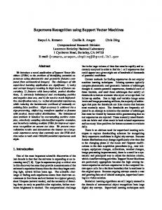
The Danish Labour Force Survey was collated in 1996 and consists of population register records. There are 15579 records measured on 14 variables7. income is the only variable missing values; 4175 records must be imputed for this variable, approximately 30% and the missing data pattern is genuine. income takes values in the range [0-1,000,000], measured in Danish Krone. The distribution is skewed, with mean 170,000 DK, standard deviation 110,000DK. A 2-dimensional plot (fig.10) shows age on the x-axis plotted against income. The dots show each respondent, the crosses show the average income for people of the given age. The circles show the mean plus and minus one standard deviation. age is clearly non-linearly correlated with income. As age increases the average income increases. A peak is reached at 50 years, after which average income declines. The variability changes with age also.

Apriori suitability of SVM Before applying the SVM to this dataset we made the following observations concerning features of the data and our expectations of success. Data size: There is plenty of data available for training an SVM. 7 in fact there are 13 informative variables response just indicates if the income value is missing

17

5

10

x 10

8

income (Danish Krone)

6

4

2

0

−2 10

20

30

40 age (years)

50

60

70

Figure 7. age vs. income

Variable types: Except for age all variables are categorical. We therefore do not expect highly non-linear correlations. Missing data pattern: Only one variable is missing. This makes application of SVM particularly straightforward.

3.1.3

Imputation

data preparation: All variables are normalised (including categorical variables and the target), to zero mean and unit variance. It is important that the length scales of each variable are similar. There are 11404 records available as training data. We use only 5000 units, as larger training showed no improvement in cross-validated error, and was slow to process. SVM setup: We applied SVM regression as income is scalar valued. An rbf kernel is chosen as we believe from figure 10 that the imputation variable may be non-linearly correlated with age and this kernel supplies non-linear models. SVM regression has three model parameters: σ, C and . These parameters are not learned during training. They must be estimated by comparing a number of settings on a validation set. We cross-validate the three parameters, each initially having five settings8 . This results in 53 = 125 different model orders being compared. We used 4-fold cross-validation, comparing rmse. Evaluation of each setting took 1 minute approximately. The experiment took 2 hours to 8 We

give the cross-validation range, and best settings in the appendix

18

complete on a DEC-Alpha with 450Mhz CPU and 40Gb of swap space. The settings for the model parameters were: C=20, σ = 6 and  = 0.1.

Simulated missing data mechanism Exploratory experiments were performed by introducing an artificial missingness pattern into the 11404 complete records. An MCAR pattern was used, deleting an income value with probability 0.3, repeating the experiment 20 times. We imputed values using a linear regressor, a neural net (MLP) and the group-mean algorithm. The neural net was a feedforward MLP from the NETLAB toolbox [13]. Group-mean variables were (3) age, (6) business type, (2) sex,(5) education. These variables partioned the input space into 160 possible subgroups. The variables were chosen incrementally. The single best variable is age, discretised into 5 subgroups. Table 1. Development Results: income SVM rbf MLP Group-mean Linear

K-S ±0.01 0.07 0.12 0.13 0.10

mae ±1000 53000 58000 61000 61000

rmse ±3000 83000 87000 90000 92000

worst case 780000 790000 810000 790000

Below we show the performance improvement for the group-mean algorithm as each variable is added. The non-linear SVM is outperforms the linear SVM on rmse. The worst case error is large, nearly 80% of the range. The rmse estimates had a standard deviation of 3000DK, the mae results had a standard deviation of 1000DK. Table 2. Development Results: Group Mean for income group-mean variables (3 6 2 5) (3 6 2) (3 6) (3) linear regressor

3.1.4

K-S 0.09 0.13 0.21 0.40 0.13

mae 57000 62000 65000 73000 62000

rmse 91000 96000 102000 115000 95000

worst case 720000 750000 790000 850000 720000

Results

In this section we present results for the Evaluation Data. These experiments were evaluated independently by ONS. Imputation of the 4175 income values originally missing from the dataset was made. The true values, extracted from

19

tax records, were retained by an independent evaluator9 . All variables were normalised before training. As well as a ‘vanilla’ application of the SVM, we investigated two refinements; variable selection and stratification. Variable selection involves the selection of the most informative variables in a step-wise additive process. The single best variable is selected first (based on a validation set, comparing rmse). This variable is then combined with all others and the best pair is chosen, then the best set of three, and so on. The best variables, in decreasing order, were age,business type, sex, marital status and employment status, the same as those chosen by the group-mean algorithm. Feature reduction can improve generalisation by removing noisy variables that might mislead the optimisation routine. SVM rbf strat denotes a stratified procedure. Two SVMs, one trained for male respondents and the other for female respondents are applied. We investigated all variables, but only stratifying on sex improved cross-validated error. The model order that was found by cross-validation was similar for all three setups; σ = 5, C=10 and  = 0.1. In the table below slope represents the weighted Pearson moment, mae the mean absolute error, rmse the root mean square error, KS the Kolmogorov -Smirnoff distance and MSE the mean squared error. We show the best results from amongst the Euredit partners. Table 3. Results: income 1 2 3 4 5

algorithm SVM rbf SVM rbf vs SVM rbf strat strat. linear DIS (hotdeck)

training size 5000 5000 5000 each class 10000

slope 0.93 0.94 0.94 0.922 0.83

mae 46000 45000 46000 47000 63000

rmse 80000 80000 80000 79000 102000

KS 0.102 0.099 0.095 0.077 0.06

MSE 1600000 1100000 1100000 1710000 3927580

The fourth model was a stratified linear model, augmenting the data with interaction and quadratic terms (age2 ). 80000DK rmse represents approximately half of the mean value for income and two thirds of the inter-quartile range which is 116000DK. A relatively weak dependency has been found. Of course this makes sense given the granularity of the input variables. The performance of the augmented linear model (4) is also informative. The technique is much less powerful than the SVM and yet was able to achieve comparable performance. Of course the technique required expertise and hand-tuning. 9 The UK Office of National Statistics. For the purposes of the Euredit Project, each participant in the project had access only to the incomplete dataset, and all results presented were evaluated independently

20

Summary There is little difference between the SVM results. The rmse, rounded to two significant figures, is identical for all three approaches. SVM does not require stratification, or feature reduction for this problem. The algorithm was able to extract a model from the data without fine tuning or apriori knowledge. The Kolmogorov-Smirnoff is a measure of preservation of distribution. It gives the maximum percentage difference between the cumulative distribution functions of the true and imputed values. The SVM scores 10%. KS=0.035 results were presented elsewhere, however this value was achieved with a rmse of 104,000DK and a mae of 64,000DK. This highlights an obvious tension. Low rmse is likely to conflict with good KS values. We achieve low rmse by predicting at the conditional expectation. However this will compress the distribution making it seem more peaked at the mode than it is. Another approach would be to compare techniques before and after the adding of residuals. In this way the ability of a model to capture the correlations would be measured, as well as the noise. We wish our imputations to contain noise, as otherwise estimates of correlations will be too large and confidence intervals too small. In the next section we consider multiple imputation. This procedure enables users of imputed datasets to reflect the underlying missingness in any statistics and confidence intervals they may calculate.

Multiple Imputation We apply the Multiple Imputation framework[17][10][18] to derive confidence intervals that are sensitive to the underlying missingness. A number k of draws from P (Y |X) are made for each missing datum10 which result in k completed datasets. Assuming we wish to calculate the mean, µ, and its confidence interval, the standard error σ(µ), we perform the standard analysis on each of the k completed datasets, producing µ1 , . . . , µk and σ(µ)1 . . . , σ(µ)k . These two sets of statistics are then inserted into the generic formulae devised by Rubin, to produce an overall estimate for the standard error σ(µ)total . This estimate should reflect the increased uncertainty due to missingness. As the SVM is limited to modelling E(Y |X), we turn to Gaussian Processes. These Bayesian models can produce estimates for the predictive distribution P (Y |X) under the assumption of gaussian noise. Recent interest in this approach has been excited by work on Bayesian neural networks[14][11]. In addition, a connection with the SVM has been made[5]; it has been shown that the mean of the predictive distribution of a Gaussian processes is identical to the SVM regressor trained with zero width epsilon-tube.

Gaussian Processes A stochastic process is a collection of random variables, {Y (x)|x ∈ X} indexed by set X. We can think of stochastic processes as arising from a distribution 10 5-10

imputations usually suffice

21

D over a space of functions, F; {Y = f (x)|f ∼ D(F)} applied to a fixed set of vectors {x ∈ X}. The stochastic process achieves an appealing generality as we do not parameterise the input-output relationship explicitly, but instead parameterise a probability model over the outputs given the inputs. This model is defined by specifying the form of the marginal distribution for the f (X) when applied to a finite set of variables. A Gaussian process is a stochastic process for which the marginal distribution over any finite set of variables is zero mean Gaussian11 . 1 Pf ∼D [f (x1 ), ..., f (xl )) = (y1 , ..., yl )] ∝ exp(− y Σ−1 y) 2

where Σ is a symmetric positive definite covariance matrix. Element Σij of the matrix describes Ef ∼D [f (xi )f (xj )], the correlation between the function outputs at the two points, xi and xj . We assume a function k(, ) that calculates the covariance of f evaluated at two points: k(xi , xj ) = Σij . The covariance function must generate a non-negative definite covariance matrix for any set of points. We imploy the following covariance function; k(xi , xj ) = exp{−

1 xi − xj 2 } 2 r2

This function captures the intuition that correlations should be high between points that lie close together in the input space. r describes the size of the ‘neighbourhood of influence’. As r increases the neighbourhood grows, resulting in a prior that favours smoother functions. We have a training sample S = (X, y) = {xi , yi }ni=1 with which we will calculate a posterior distribution over the function space. We assume that each label yi is equal to an output value ti corrupted with Gaussian noise (mean zero, variance λ2 ). 1 P (y|t) ∝ [− (y − t) Iλ−2 (y − t)] 2

This assumption allows us to derive a Gaussian form for the distribution we desire: P (t|z, S), the distribution for the output t for a new test point z, given the training set S; S. P (t, t|z, X) = P (t, t|y, z, X) =

P (y|t, z, X)P (t, t|z, X) ∝ P (y|t)P (t, t|z, X) P (y|z, X)

The denominator is ignored, as it does not depend on the choice of hypothesis. The first factor P (y|t) is the weighting given to a particular hypothesis identified by its output values on the training set inputs.  We marginalise over t: P (t|z, S) = P (y|t)P (t, t|z, X)dt. A useful feature of a Gaussian process is that this predictive distribution is also Gaussian and an exact analytic form can be produced using matrix manipulations[11]. The mean and variance of the predictive distribution are given by: f (z) = y (Σ + λ2 I)−1 kz V (z) = k 11 This

zz

z 

2

− (k ) (Σ + λ I)

presentation is based on [5][11]

22

−1

(15) k

z

(16)

where Σ is the covariance matrix, kzi = k(z, xi ), the vector resulting from the kernel applied to each training point and the test point and kzz = k(z, z), the covariance of the test point with itself. V (x) estimates the variance at each prediction point. We generate multiple imputations by calculating the mean of the missing value using f (z) and adding gaussian residuals of variance V (z).

Multiple Imputation Experiments We estimate the standard deviation of the mean of DLFS income variable under an MCAR missingness pattern, with rate 30%. There are 7000 observed values and 3000 imputed. The noise parameter λ and the parameter r (for the covariance function) are found by cross-validation. For normalised data λ = 2, r = 0.35. Results presented below show the confidence intervals for the mean estimated with 10 multiple imputations drawn from the Gaussian process. We calculate the intervals at the 90, 95 and 99% levels. As the missing data mechanism is MCAR, we know that the mean has standard deviation, √ σ , where no bs is (nobs )

the number of the observed data ans σ is the sample variance. Table 4. Results: Multiple Imputation algorithm true svm

90% 1700 1400

95% 2100 1800

97.5 2600 2200

99% 3000 2600

The Kolmogorov-Smirnoff measure for a singly imputed dataset with a GP gave 0.7, and improvement of 30% over the SVM, although not nearly as good as the best result. We show that the confidence intervals calculated by the GP give too small confidence intervals at the 90%,95% and 99% levels, by a factor of a fifth. This shortfall is due to the Bayesian model for the noise being incorrect. Observation of figure 10 shows that skewed noise.

23

3.2 3.2.1

Dataset SARS: Sample of Anonymised Records Technical Summary

Method: Data: Training Dataset: Hardware used: Software use: Test scope: Preprocessing: Training-data size: Processing time Set up time: Training: Testing time: Total: Full Total:

3.2.2

SVM regression, classification, multiclassification ‘newhholdm’ Sample of Anonymised Records Y2 A subset of complete units DEC Alpha UNIX mainframe. MATLAB 6.0 and C code Imputation only normalisation, design variables. multiclass: 2000 units in each class, regression: 3000 units total (per variable) 5 minutes 120 mins. 5 mins. 130 mins. × 25 variables = 2 days.

Data Description

The data is a 1% sample of household records from the 1991 UK census, totalling nearly half a million records. Each row represents one person and each item on the row describes a feature of the house they live in or their job and education. For example one variable describes the number of rooms in the person’s house, another the number of qualifications they have. The exact number of records is 492,472. There are 31 variables in total. Two of the variables are treated as scalar; age and hours worked. Two variables are binary valued: sex and ltill. All other variables are multi-class discrete valued. Table 5. Evaluation Data: #Missing items for each variable. HHSPTYPE 29045

ROOMSNUM 33516

TENURE 25821

AGE 39150

DISTWORK 12103

HOURS 16638

LTILL 34511

MSTATUS 49409

RELAT 29829

RESIDSTA 39348

QUALNUM 29578

QUALEVEL 3161

QUALSUB 3172

SEX 34586

WORKPLCE 12319

ECONPRIM 12801

ISCO2 26086

ISCO1 26086

The dataset is hierarchical: the census questionnaire contains a section relating to the household and a separate section for each household member. In order 24

to create a rectangular data matrix12 , the data is tabulated with the household information copied to each respondent. Values (and missingness) for the household variables are therefore identical for each household member. Household variables should therefore be imputed identically for all members. The imputation problem is posed in two forms; the ‘Y2’ form with missing values, and the ‘Y3’ form with errors and missing values. We attempt imputation of both. Cleaning of Y3 is limited to removal of out-of-range values, no edit rule checks are made. Variables have a relatively low rate of missingness. In table 6 we describe the missingness pattern. 33% of rows are missing no items, 34% are missing one item, and so on. Table 6. Rate of missingness for SARS #missing % rows

0 33

1 34

2 20

3 9

4 2

5 1

6-9 1

We note that ISCO1 is derived from ISCO2 and thus has identical missingness pattern. Naturally this means that one cannot be used as an input variable for the other. Various other relationships between variables are also known apriori through common sense. For example age will dictate whether the respondent has a job. If age is less than 16, the variable ISCO will take the value ‘not applicable’. Such clear-cut relationships can be conveyed through edit rules and logical or deductive imputation may be possible. Evaluation Data and Development Data The full experiments are performed on SARS ‘evaluation data’ consisting of records from region 1 and regions 3 to 12. For these experiments Euredit partners are issued only the incomplete data, ONS retaining the true values. Imputed datasets are returned to ONS for independent evaluation. In addition to the evaluation experiments exploratory experiments are performed on a portion of SARS data collated in region 2, known as ‘development data’. This dataset contains 45,000 records, with missingness as described in table 7. This data is considered large enough for useful comment to be made. For the development data we are issued with both the complete dataset and a version with missing values and errors. We are thus able to to evaluate performance ourselves. On this smaller dataset we obtain estimates of relative performance by comparing the SVM with a group-mean benchmark. See the appendices for a description of the group-mean benchmark algorithm. It operates similarly to DIS. We note that the Wald statistics is proportional to the size of data imputed. If we calculate the Wald statistic for a dataset consisting of the conjunction of 12 We make the dataset rectangular as this makes handling by standard software more straightforward.

25

Table 7. Development Data: Missing items for each variable HHSPTYPE 2558

ROOMSNUM 3970

TENURE 2150

AGE 3623

DISTWORK 1147

DISTWORK 1147

HOURS 1548

LTILL 3185

MSTATUS 4624

RELAT 2728

two identical copies of the data, it is twice the value of the original. As the evaluation data is 11 times the size of the development dataset, we therefore expect the Wald statistic to be 11 times bigger.

A priori suitability of SVM SARS has various features that we know to be relevant to the set-up procedure and our expectations of success. Before imputing with the SVM we made the following observations. Variable types: Most variables are categorical, and the dimensionality (31 variables) is relatively low. In addition, there is a vast amount of data available. From such characteristics we can infer that non-parametric methods are likely to perform well. It would therefore be sensible to compare any semi-parametric method with a non-parametric method, such as DIS. Especially as such approaches are more transparent. In addition we note that many of the variables contain low frequency classes. Donor methods naturally maintain the frequencies of these classes. SVMs ignore rare classes in any region where they are not modal. Missing data pattern: The low rate of missingness (see table 6 above), favours the application of SVM. Only 13% of units lack more than 2 values. See section 2.4 for a description of how we handle missing input variables. When the missingness rate is low a ‘quick and dirty’ method was deemed acceptable: we ‘estimate’ each missing input variable, using its mean. Training data: SVM training requires the solution of a convex quadratic programme, a computationally expensive task scaling with O(n3 ). SARS contains approximately 100,000 complete records. This is more training data than our SVM implementation can handle, however it is almost certainly more than the task actually requires. We can learn the correlation adequately from a few thousand data points. We use as much data as can be handled in a timely fashion. For regression we use 3000 units, for classification 2000 per class. Given the low dimensionality and simple correlations it is unlikely that this policy leads to significantly poorer results. 26

Hierarchical structure: Members of one household are correlated, for example, spouses will typically be of similar age. This means that the rows are not independent and identically distributed (iid). More importantly strong correlations between household members will not be learned by the SVM. We note that over 10% of households contain only one person however. An optimal strategy may be to impute these units using the SVM, and to use appropriate heuristics for larger households where correlations between household members can be exploited.

27

3.2.3

Imputation

Data Cleaning: Values out of range were removed. Very rare classes (less than 1% of training size) were removed as the SVM cannot train with extremely unbalanced data. Variable Selection: We use all variables for training, apart from index variables. It is noted that some variables are derived and are therefore always mutually absent (e.g. ISCO1, ISCO2). Therefore we do not train with ISCO1 when predicting ISCO2 and vice versa. Preprocessing: Normalisation of all variables is carried out. This leads to each input variable having comparable influence. Model parameter settings: We apply an SVM with ‘rbf’ kernel. Our aim is to evaluate this kernel as a generic non-linear SVM model. See section 2.2 for a discussion of other kernels. We apply SVM classification and regression to SARS. The error trade-off parameter C and σ (the kernel parameter) are set by cross-validation for both types. For scalar variables,  (the width of the ‘tube’) is also set by crossvalidation. Below in table 8 we give the ranges of values. C values that gave good performance were low (5 and 20 for most variables) indicating that training error was high. The kernel parameter, σ normally lies in the range [ d4 , d], where d is number of input variables. Table 8. Cross-validated settings parameter settings σ 8 12 16 20 24 C 5 20 80 300  0 0.01 0.05 0.1 0.2 # cross-validation settings = 5 × 4 × 5 = 100

Training data selection For training data we select units that lack no values at all. At least 30% of the data is complete. For regression we take 3000 units. For (multi)classification we select 2000 units in each class maximum. If the classes are unequally sized, we draw proportional to the ratio. I.e. if class 1 appears twice as often as class 2, we pick 2000 of class 1 and 1000 of class 2. This may lead to the deletion of very rare classes from the training set. For example, the 4th variable bath indicates whether the household has exclusive use of a bathroom (1) , shared use (2) or none at all (3).The relative frequencies of these values are; 100 : 0.7 : 0.01. Less than 1% of people share a bathroom. Less than one in ten thousand have no bathroom at all. It would distort the distribution to include respondents with no bathroom. In any case, it is unlikely that there is any region of input space where this value is modal. 28

3.2.4

Results

We present results for the scalar variables first, and then consider selected discrete variables. Comparison is made with results from EUREDIT partners who used standard methods. In addition to the full-scale experiments evaluated by ONS, we present results of exploratory experiments performed on ‘Development data’, a labelled portion of the data containing 45,000 units. We were able to evaluate experiments on this smaller subset quickly ‘in-house’, and estimate performance. The scalar variables are age in years and length of working week in hours. These variables bear obvious relationships with others in the dataset. For example, all children will have zero for hours worked. The variables ISCO and econprim will also be informative for these variables. We tabulate the Pearson correlation coefficient (slope), the mean absolute error (mae), the root-mean-square-error (rmse), the worst-case error (worstcase) and the Kolmogorov-Smirnoff measure (K-S).

Imputation of AGE In figure 8 we plot the two regression variables against each other. The number of hours worked is (non-linearly) correlated with age. The dark line represents the average number of hours worked for each year-group, the lighter lines show plus and minus one standard deviation. Figure 8. age vs. hours AGE versus average HOURS 60

50

HOURS WORKED per WEEK

40

30

20

10

0

−10

−20

0

10

20

30

40

50 AGE

60

70

80

90

100

Many people in the age range 16-20 are in higher education and so reduce the average working week. Similarly early retirement leads to a gradual overall reduction in the average hours worked per week. All respondents in the age 29

range 71-80 are recorded as having 71 years. Similar grouping is supplied for the subsequent decades. This explains the sharp peaks at the upper end of the graph. Development data: As a reality check the group-mean approach (described above), was evaluated using grouping variables econprim and relat. This approach yielded a rmse of 11, and a KS value of 0.19. The SVM produced a result of 9 and 0.092. The simple benchmark is not much worse than the SVM. In another exploratory experiment we imputed all household-heads with their spouse’s age plus two (for those respondents who had a spouse). This gave a rmse of 4.4. Similarly we imputed each child with the household head minus twenty-eight. This yielded a rmse of 6.1. These household dependent heuristics perform better than the SVM by a large margin. Evaluation data: Table 9 presents results for the evaluation data and compares with DIS. The SVM preserves the true values much better than DIS. Table 9. Evaluation Results: age Partner ONS RHUL

Algorithm DIS SVM(rbf)

slope 0.85 0.86

mae 11.3 6.5

rmse 17.5 9

worst-case 95 91

KS 0.13 0.10

Neither DIS nor SVM exploit heuristics based on household structure. The SVM outperforms the standard method, but results on region 2 data indicate that household dependent heuristics will perform better still.

Imputation of HOURS This variable records the number of hours worked per week. It takes values in the range [1-81]. ‘Inapplicable’ is denoted by -9, and used for children for example or retired people. It is possible that this variable would be better imputed in stages. First -9 values using a classifier and then a regression for the other variables. We took a naive approach and imputed everything with SVM regression. Development data: Imputing 1548 items, Group-mean with variables ISCO1 and econprim achieved rmse of 9.3 and KS equal to 0.34. The SVM achieved rmse of 12 and KS = 0.24. Evaluation data: Results in table 10 show the SVM to offer an improvement over the DIS for preservation of true values. The Kolmogorov-Smirnoff measures are similar however.

30

Table 10. Evaluation Results: hours Partner ONS RHUL

Algorithm DIS SVM(rbf)

slope 0.91 1.03

mae 16.5 9.5

rmse 25 13.9

worst-case 90 81

KS 0.25 0.26

Imputation of SEX For all discrete valued variables results are given for the Wald-statistic (W), and the error rate (D). For both of these statistics, less is better. The sex variable is self-explanatory. One would expect heuristics that exploited the household structure to be successful. Development data: The group-mode with covariates ISCO2 and econprim imputed 315 subgroups, achieving an error of 0.28 and Wald-statistic of 80. Evaluation data: Results in table 11 show the SVM with rbf kernel outperforming DIS on both measures. Table 11. Evaluation Results: sex Partner ONS RHUL

Algorithm DIS SVM(rbf)

W 654 22

D 0.33 0.27

Imputation of MARITAL STATUS This variable takes five values. The first two classes occur much more frequently than the last three. Table 12. Classes: marital-status value meaning %freq

1 single 40.5

2 married 41.5

3 remarried 5.5

4 divorced 4.5

5 widowed 7

There may be no regions where classes 3-5 are modal. Hence predictive techniques like SVM will not impute to these classes. As a strategy for minimum error rate this is correct, for preservation of the marginal distribution it is incorrect.

31

Development data: The group-mean achieved an error rate of 0.16 and a Wald-statistic of 260. We used variables relat, persinhh, age(discretised) and econprim. Evaluation data: For this data the SVM has provided lower error, but not preserved the distribution well. It is probable that the smaller classes are never modal, and therefore are not imputed to. Table 13. Evaluation Results: marital-status Partner ONS RHUL

Algorithm DIS SVM(rbf)

W 919 2900

D 0.32 0.19

The benchmark results point to the existance of simple relationships readily exploited by the group-mean algorithm.

Imputation of LTILL ltill is a binary variable. Just over 1 in 10 respondents are long-term sick (14%). Missingness occurs at a rate of 10%: approimately 40,000 items are missing. The 27th variable econprim encoding the ‘Primary economic position’ is closely related to ltill. If econprim has value 8 (permanently sick) then ltill has value 1 with probability > 0.99. Development data: The group-mean with variables econprim, age and marital− status, achieving D=0.11, W= 270. If we use econprim alone, we achieve an error rate of 11%, and a Wald-statistic of 350. DIS offers better preservation of marginal distribution. Evaluation data: Results presented in table 14 show the SVM to have discovered a dependency, but to have preserved the distribution less well than DIS. Table 14. Evaluation Results: ltill Partner ONS RHUL

Algorithm DIS SVM(rbf)

W 211 740

D 0.17 0.12

Imputation of RELAT This variable describes the respondents relationship to the household head. ‘0’ indicates the household head themselves, ’1’ their spouse and so on. Values are 32

in the range [0-16]. The classes are of very different sizes, the table below gives percentage frequencies. The most common values (> 1% frequency) are shown in table 15. Common sense informs us that certain variables will be correlated with relat, for example age. Table 15. Classes: relat value meaning %freq

0 head of household 41

1 spouse 22

2 cohabitee 3

3 son/ daughter 31

4 child of cohabitee 1

5 etc ... ...

Development data: The group-mean benchmark attained D=0.17 and W=163 with variables sex, maritalstatus, age and econprim. We applied the SVM to the same subset of data. This attained a much lower error rate than the groupmean benchmark, scoring D =0.07, W = 43%. Investigation revealed that the variable pnum was strongly predictive for the SVM. When this variable was added to the group-mean variables, performance improved to the same level as the SVM. Common sense might have told us that the head of the house completes the questionnaire and will thus submit their details first, then their spouse and children. However, this kind of correlation is due to the way the information is acquired, and seems ‘accidental’. It is clear that manual variable selection might well miss this type of dependency. Ultimately the performance of the group-mean and the SVM are close for this exploratory experiment. Moreover, an automated variable selection strategy would have discovered the value of using pnum for the group-mean algorithm. Evaluation data: In table 16 we present results for the evaluation data, and compare with those from DIS. Table 16. Evaluation Results: relat Partner ONS RHUL

Algorithm DIS SVM(rbf)

W 1286 232

D 0.354 0.07

The optimal imputation of age involved use of domain knowledge. This might hold for this variable, although error here is already low. Clearly, if another record in the household has relat value 0(= head of household), then it is fair to deduce that the given record will not have this value. Similar inferences concern the value for spouse.

33

The SVM with rbf kernel performs near to the optimal. It is notable how much the results exceed that of the Donor Imputation System (DIS). This is because the variable pnum was not used as a covariate. Our group-mean algorithm was able to attain much improved performance using this varible, and its approach is very similar to that of DIS.

Imputation of HHSPTYPE hhsptype takes values in [1-14]. There is an ordering in these values, but the variable is treated here as categorical. 20% of units take value detached, 40% are semidetached, 30% are terraced, and 6% are residentialf lats. All others categories together make up the remaining 4% of units. Development data: The benchmark algorithm, using variables rooms, tenure and persinhh achieved D= 0.57, W= 980 on region 2. Imputations are wrong more than half of the time. The SVM achieved D=0.514, W = 108. Observation of the cross-tabulated imputations and true values showed that classes 1 and 3 overlapped to a degree of 25%. A large number of class 1 and class 3 values were imputed as class 2 however. Although class 4 was smaller its frequency was well preserved. The comparable error rates indicate that a simple correlation underlies exists between hhsptype and the other variables. Evaluation data: In table17 we see the SVM error tallies with those estimated on region 2, and are comparable with other results for D. SOM achieved better performance for the Wald-statistic, but slightly worse error rate. By reassigning class 2 predictions to class 1 and 3 we could improve our Wald-statistic at the expense of a higher error rate also. Table 17. Evaluation Results: hhspace Partner ONS RHUL

Algorithm DIS SVM(rbf)

W 970 1620

D 0.71 0.56

Imputation of TENURE tenure is a categorical variable with values in the range [1-7]. In table 18 we tabulate the meaning and frequency of occurence of the possible values. The class sizes are unbalanced. Development data: The group-mean benchmark was used with 3 variables; hhsptype,age and econprim, where the last two variables relate to the household head. This simple algorithm achieved D= 0.38 and W=200 on region 2, where

34

Table 18. Classes: tenure val. mean. %freq.

1 own outright 21

2 own buying 49

3 priv. rent. furnish. 3

4 priv. rent. unfurn. 3

5 rent. job 1

6 rent. hous. assoc. 1

7 rent. publ. sector 22

2150 items were imputed. We ran the SVM on the same subset of data and achieved an error rate of 0.36 and a Wald statistic of 257. Classes 4, 5 and 6 were largely ignored, hence the large Wald statistics. The SVM does not outperform the much simpler technique. Evaluation data: Below we present some selected results from the full dataset experiments. Complete tables can be found in the appendices. The SVM has learned the dependency reasonably well. Table 19. Evaluation Results: tenure Partner ONS RHUL

Algorithm DIS SVM(rbf)

W 1800 3000

D 0.62 0.35

The error and Wald-statistic tally with our estimates from region 2. The good error rate also indicates that the SVM has found whatever correlation exists in the data.

Imputation of ROOMS The variable rooms counts the number of separate rooms in the house and lies in the range [1-16]. However table 20 shows that the distribution is strongly skewed. The low frequency values at the top of the range will be ignored by predictive methods. Table 20. Classes: rooms #rooms %relative freq

1 2

2 8

3 17

4 27

5 22

6 17

7 4

8 2

9 -16 1

Development data: The group-mean benchmark used 3 variables: persinhh, hhsptype and ISCO1, where the last two variables relate to the household head. All members of the household are imputed identically on household variables. This benchmark achieved D= 0.67 and W=798. 35

Table 21. Evaluation Results: rooms Partner ONS RHUL

Algorithm DIS SVM(rbf)

W 970 5500

D 0.70 0.66

Evaluation data: In table 21 we present results for the SVM and DIS. Error rates are comparable, but the SVM performs worse on marginal distribution. Donor methods are better able to preserve rare classes than predictive methods.

Summary of SARS results Preprocessing: We do not investigate more sophisticated variable selection. However it is possible that this would be beneficial. For example, we could remove household variables for imputation of individual variables. Training phase: We can build an adequate model with a small percentage of the training sample available. Validation on training sets of size 500, 1000, 2000 etc showed small improvement over 1000 units. Training and validation times were about 60 minutes for each variable for 100 settings. The full dataset required over a day to process. Rare classes caused some practical problems. More than 4 samples are required for 4-fold cross-validation of course. In fact 20 or 30 instances are required if the data is separated randomly. When there were not enough we deleted the rare classes. In some cases we deleted the variables altogether. Test phase: The SVM test-phase is linear in the number of points to estimate. Once the SVM is trained, imputing 1,000 values requires less than 10 seconds with our implementation. For this dataset, where there are about 1 million missing items in total, the test phase takes approximately 3 hours. Performance: We have tabulated results for the following variables; age, sex, ltill, marital − status, relat, hours, tenure, hholdtype and rooms. The SVM was in the top two or three for preservation of true values for all of these variables. The performance on relat was excellent. Where a dependency existed, the SVM finds it reliably, both for scalar and categorical variables. Given that no variable selection was performed or stratification this result is remarkable. SARS scalar variables: KS measure The results are not conclusive for the preservation of marginal distribution. KS measure for age and hours was average to poor, but not outstandingly bad. We know that the SVM imputes at the expected value in the case of scalar variables. This will remove noise from the dataset, and result in a ‘compression’ of the distribution.

36

SARS discrete variables: Wald Statistic The W measure for categorical variables was never the worst and for sex was close to the optimal. However, if correlations are weak we have no reason to expect good preservation of marginal distribution. The effect of imputing the maximum aposteriori class will be to compress the distribution. In this respect the SVM can only be optimal if there is no noise at all: if P (Y |X) has a peak at the expectation, and zero height elsewhere. The compression effect can be lessened by adding residuals to the predictions. This has not been investigated here. Hierarchical structure: The census is a hierarchical dataset. Within a household the distribution of each member is dependent on the other members. For example, the age of a child will be strongly correlated with the age of a parent. The SVM system applied here does not exploit this structure. The SVM assumes each row is i.i.d. Results obtained by Statistics Finland for the age variable show that such relationships can be usefully exploited. When compared with with other algorithms not exploiting data-dependent heuristics, the SVM performed reasonably for this variable. It should also be noted that 10% of the households have only one occupant. For these respondents no household heuristics can be used. SARS Y3: Tables are given in the Appendix for SARS Y3. Results were comparable with SARS Y2. The perturbations did not seem to strongly affect the performance of the algorithm.

37

3.3 3.3.1

ABI: Annual Business Inquiry Technical Summary

Method: Training data set: Hardware used: Software used: Test scope: Editing of Y3: Processing time for each variable: set-up time: cross-validation: 125 * 4-fold * 30 secs training time testing time TOTAL per variable

3.3.2

SVM Regression Imputation Completed portion of ABI Sector 1 1998(Y2) DEC Alpha UNIX MATLAB, SVM in C-code Imputation only None performed. 5 minutes (125 settings) 250 minutes 1 minute 0.5 minutes 4.5 hours

Data description

This dataset contains information concerning 6233 businesses, each having completed a questionnaire known as the ‘Annual Business Inquiry’. The questionnaire concerns various financial characteristics such as expenditure on personnel or equipment. Each row in the dataset is a business, each column contains an answer to one of the questions. ABI has two questionnaires with one (the ‘short’ version) only asking for summary information. Variable values for questions not on the short form are set to (-9) for businesses answering the short form. There are four ‘reference variables’ acquired independently from the dataset. The dataset exists in two forms, Y2 which is missing values, and Y3 which is missing values and also contains perturbed or erroneous values. We performed experiments on both datasets. We do not attempt to clean the Y3 data. We reduce the dimensionality of this dataset to 16 variables for the imputation process. We chose those variables common to the long and short form questionnaires and the fully observed reference variables as well ref ,class,weight, turnreg, empreg and f ormtype13 . All of the imputation variables are non-negative scalar valued, representing sums of money, with the exception of employ and empreg, which encode the number of employees. There are a few records far removed from the others in the input space. These can be called ‘representative outliers’; correctly measured units with some variables taking values very much larger than all the others. These records are for multi-nationals. Below we show a histogram of log(TURNOVER+1) partitioned in 10 bins. The skewness of the marginal distribution of TURNOVER 13 An

appendix contains the meta-data file.

38

6

10

PURTOT vs. TURNOVER

x 10

9

8

7

6

5

4

3

2

1

0

0

2

4

6

8

10

12

14 6

x 10

Figure 9. purtot vs. turnover
n is apparent. We calculate the third moment; m3 = n1 i=1 (xi − mean(x))3 to get a measure of the skewness. For TURNOVER, m3 = 7e+17. log(turnover+1) 1500

1000

500

0

0

2

4

6

8

10

12

14

16

Figure 10. log(turnover)

Missing data pattern The data contains 6233 records of which over 4000 are completely observed. In Table 22 below we show the number of units with no variables missing, one variable missing and so on. This is a relatively benign pattern. Of the 1052 units that are missing values, only one tenth have more than one value missing. There in total 85 different missing data patterns. It is therefore feasible to train a separate SVM for each. Table 22. sec298y2 missing data pattern num. missing in row num. of units

0 4932

1 1052

39

2 135

3 27

4 67

5 18

6 2

3.3.3

Imputation Setup

Selection of data for training For training we select 3000 units from the fully observed portion. This number can be handled in a timely fashion. Preprocessing The index and weight variables were deleted before training. All remaining variables were normalised. No log transform was used. No stratification was used. No editing was performed in the main experiments. Regression was used for all variables. The SVM was evaluated as an automated tool and therefore we wished to do a minimum of preprocessing. Model Order All experiments are performed with an rbf kernel. This kernel has one parameter, σ. The other model parameters, C and  are found by crossvalidating the settings shown in Table 23. We compare 125 models in about 4 hours. Table 23. Cross-validated settings parameter σ C 

settings 3 6 9 12 15 2 5 10 20 100 0 0.01 0.05 0.1 0.2 1

Our cross-validation routine compares models with respect to the root-meansquare-error(rmse). When the best setting includes a top or bottom value (e.g. 15 for σ), we evaluate more settings (e.g. σ = 20, 25, 30...). Ultimately very low capacity models are chosen, close to linear. The parameter σ is more than 200 for all variables apart from assacq. Optimal C is 500; also relatively high. The tube width  was 0.01, or 0 for most variables indicating low noise. Due to the skewness of the data, the normal range of σ was not effective. This kernel parameter normally takes values less than the dimension of the input space. As σ grows the global influence of each data-point gets larger.

3.3.4

Results

We imputed variables common to the short and long forms that were missing values. In this section we give results for T U RN OV ER, EM P LOY , ASSDISP and ASSACQ. Full results are given in the appendices. In addition to the results evaluated independently by ONS (in Tables 26,29,38 and 35) we give results for ‘development’ experiments. We took the fully labelled portion of the sector 2 1998(Y2) dataset and used half for training and half for testing. This allowed us to evaluate various models in house and make estimates for performance. We make comparison with linear techniques

40

Imputation of TURNOVER TURNOVER is a scalar variable, describing the total turnover of the company in the year 1988. In Table 24 are some statistics taken from the fully observed units in the ABI Y2 evaluation data. The distribution is clearly skewed. ABI contains records for multi-nationals and businesses with just one employee. Table 24. Summary: TURNOVER range [0-1.3e7]

mean 18,699

variance 7e10

median 276

inter-quart. [110-1028]

95% range [0-24735]

TURNOVER is correlated strongly with ’TURNREG’ (0.986), ’PURESALE’ (0.995) and ’PURTOT’ (0.998)14 , where the Pearson correlation coefficient is given in brackets. Using these variables we performed an exploratory experiment on the fully observed portion of the data (4932 rows). Half of the data was used for training and half for test. Linear regression was performed using the three variables above with highest correlation. The experiment was repeated with a log transform of all variables. The results below show that good preservation of true values is possible, and that a log transform helps to improve KS performance by reducing the effect of the larger values. Table 25. Development results: TURNOVER (linear regression) Vars 14, 6, 7 log 14, log 6, log 7

slope 0.998 0.998

mae 255 131

rmse 15800 24800

worst-case 22400 33000

KS 0.575 0.024

The missing-data pattern is ‘benign’. When TURNOVER is absent (136 units), variables PURESALE and PURTOT are observed in all except five cases. TURNREG is never missing. We therefore expect to do a good job of preserving values with linear regression. Nevertheless a non-linear SVM was used. We wish to know how well an automated procedure functions. Table 26. Evaluation results: TURNOVER Experiment CA2001 R2005 R2008 OA2001

algorithm Lin Reg. SVM(rbf) SVM (rbf) DIS

slope 0.9 1.14 0.97 0.40

mae 130 480 690 1100

rmse 3400 4000 1600 48000

worst-case 8100 15000 8300 113000

KS 0.05 0.76 0.67 0.14

m1 60 60 620 860

m2 2e10 2e8 6e7 5e9

The results from multivariate linear regression (CA2001) are the best of those 14 see

the appendices for a description of these variables

41

presented. For SVM the KS measure shows poor performance(log transform was not used), but all other measures are comparable with the CA2001. In summary, the problem does not seem to require more than linear regression. We expect the SVM to learn some of the noise and so perform slightly worse than standard linear methods. If good KS measure is desired, log transforms should be used. Our patching heuristic for missing input variables is naive, but few test units needed to be patched.

Imputation of EMPLOY EMPLOY is an integer valued variable, describing the number of people employed at the business. It will clearly be correlated with the reference variable, EMPREG, which is fully observed. EMPREG is an ordinal valued variable however. The integers [1-6] each represent an interval, for example 1=0-9 employees. EMPREG and EMPLOY are therefore not linearly correlated. Table 27. Summary: EMPLOY range [0-131368]

mean 232

variance 8300000

median 5

inter-quart. [2-17]

95% range [350]

EMPLOY is also correlated with EMPTOTC(0.981), TURNOVER(0.977) and PURTOT (0.967), where the Pearson correlation coefficient is given in brackets. We performed exploratory experiments as described in the section for TURNOVER. Table 28. Development results: EMPLOY (linear regression) vars 7, 4, 5 log 7, log 4, log 5

slope 0.980 0.801

mae 8.592 12.211

rmse 1206.609 3299.477

worst-case 1612.206 4787.297

KS 0.773 0.243

Log transform greatly reduces KS error at the expense of increasing rmse and mae. We expect the SVM to beat these results as it can exploit the non-linear dependency of EMPREG. The missing-data pattern is ‘benign’ for this variable. The correlated covariates are missing once in the units that must be imputed. There are only 27 values missing. Estimation of input variables is less of an issue. We therefore expect to do a reasonable job of preserving values with a linear technique. Preservation of true values is possible as strong correlations exist in the data. The results from multivariate linear regression (CA2001) and from the DIS are the best here. SVM performed worse than the donor method on all measures, and comparably with the linear regression (CA2001). The SVM with rbf kernel is expected to perform similarly to the linear regression when the spread parameter σ is large. Log transforms were not used. 42

Table 29. Evaluation results: EMPLOY experiment CA2001 R2008 OA2001

algorithm Lin Reg. SVM (rbf) DIS

slope 1.11 0.38 0.86

mae 4.2 7.9 5.3

rmse 72.20 66 28

worst-case 161 148 53

KS 0.38 0.46 0.08

m1 1 4.43 1.9

m2 15000 14000 7000

The KS value and the reasonable rmse indicate that outliers have had a strong effect on the model. The mae is high when compared with the others.

Imputation of TAXTOT TAXTOT is a scalar variable, describing the total cost of all capital assets acquired. The statistics presented below show the variable to be skewed. Table 30. Summary: TAXTOT range [0 124112]

mean 303

variance 1.2e7

median 4

inter-quart. [1-14]

95% range [369]

TAXTOT is correlated strongly with ’TURNOVER’ (0.873), ’STOCKEND’ (0.884) and ’EMPLOY’ (0.906)15 , where the Pearson correlation coefficient is given in brackets. Using these variables we performed an exploratory experiment on the fully observed portion of the data (4932 rows). Half of the data was used for training and half for test. Linear regression was performed using the three variables above with highest correlation. The experiment was repeated with a log transform of all variables. The results below show that good preservation of true values is possible, and that a log transform helps to improve KS performance by reducing the effect of the larger values. We ran an SVM with and without taking a log of the variables. The effect was less marked than for linear linear regression (which performed better on most measures). The KS measure was improved considerably. Table 31. Development results: TAXTOT vars lin reg lin reg SVM rbf SVM rbf

slope no func 4, 10, 13, log 4, 10, 13, log all vars

mae 0.427 0.963 0.901 0.604

rmse 43.308 10.321 25.427 22.392

worst-case 1851.880 2211.953 10377.535 4052.936

KS 2369.338 3520.825 16788.018 5148.043

0.962 0.293 0.246 0.359

The missing data mechanism is benign. 127 values are to be imputed, and on only 11 occasions is one of the correlated variables missing, never more than one. 15 see

the appendices for a description of these variables

43

The results below represent a selection from those produced for the EUREDIT project. Table 32. Evaluation results: TAXTOT partner OA2001 RA2008 CA2001

algorithm DIS SVM (rbf) Lin. Reg

slope 0.51 0.18 1.0

mae 8.1 12 3.4

rmse 97.3 34.1 10.4

worst-case 190 363 30

KS 0.10 0.63 0.29

m1 3.6 8.0 0.6

m2 24000 269 134

SVM results are poor. Given the successful application of linear techniques this might be due to not using log transform of input variables, or the fact that sampling weights were not used in training the SVM.

Imputation of ASSACQ ASSACQ is a scalar variable, describing the total cost of all capital assets acquired. It is strongly skewed upwards. Table 33. Summary: ASSACQ range [-9- 573,415]

mean 751

variance 1.5e8

median 0

inter-quart. [-9-12]

95% range [804]

ASSACQ is correlated with TURNOVER(0.951), TURNREG(0.963) and EMPTOTC(0.967), where the Pearson correlation coefficient is given in brackets. We perform an exploratory experiment using the fully labelled portion of the dataset as described for TURNOVER. Linear regression was performed with three variables most strongly correlated with ASSACQ. Table 34. Development results: ASSACQ (linear regression) vars no func 4, 14, 5, log 4, 14, 5,

slope 0.639 0.626

mae 113.935 51.498

rmse 3566.615 15671.005

worst-case 3814.209 23121.884

KS 0.976 0.702

The missing-data pattern is relatively benign for this variable. There are 200 missing ASSACQ values. TURNOVER is missing just 5 times with ASSACQ and EMPTOTC just once. The results for the real missing data pattern are shown below. SVM has performed reasonably on some measures. The DIS is superior on most however. The performance of the linear algorithm is less good. It seems possible that this variable is non-linearly correlated with some of the others in the dataset. 44

Table 35. Evaluation results: ASSACQ partner OA2001 RA2005 CA2001

algorithm DIS SVM (rbf) Lin. Reg

slope 1.25 1.8 3.8

mae 50 90 115

rmse 1678 3700 6000

worst-case 4773 10300 17600

KS 0.3 0.19 0.09

m1 25 33 105

m2 2.2e7 3.9e7 6.2e7

Imputation of ASSDISP ASSDISP is a scalar variable, describing the total proceeds from captial asset disposal. It is strongly skewed upwards. Table 36. Summary: ASSDISP range [-9 255615]

mean 114

variance 1.4e7

median 0

inter-quart. [-9 0]

95% range [44]

The completed portion of ASSDISP contained one very large outlier. This was removed before modelling. The remainder of the data is correlated with TURNOVER(0.812), PURESALE(0.813) and PURTOT(0.817), where the Pearson correlation coefficient is given in brackets. We perform an exploratory experiment using the rest of the fully labelled portion of the dataset, totalling 4931 units. Experiment is as described for TURNOVER. Log transform does not help here. Visualisation of the data split by CLASS and EMPREG shows these variables to be important. We expect to improve upon the results below therefore. Table 37. Development results: ASSDISP vars no func 4, 6, 7, log 4, 6, 7,

slope 0.668 0.093

mae 8.801 11.859

rmse 587.563 952.464

worst-case 622.362 1250.552

KS 0.874 0.908

The missing-data pattern is relatively benign for this variable. There are 152 missing ASSDISP values. The three covariates above are missing on 20 of these units, but only ever one at a time. The results for the real missing data pattern are shown below. Development results were reasonably indicative. 50% of values are zero, and this has not been well preserved. As a result SVM KS results are poor. Visualisation of the problem indicates that stratification by class may improve imputation of zeros.

45

Table 38. Evaluation results: ASSDISP partner OA2001 RA2005 CA2001

3.4

algorithm DIS SVM (rbf) Lin. Reg

slope 0.59 0.02

mae 6.9 10.3 3.46

rmse 109.3 157.1 56.6

worst-case 265.6 384.7 131.8

KS 0.27 0.46 0.09

m1 0.92 2.99 1.94

m2 45000 24000 14200

Strengths and Weaknesses

We have performed experiments on three datasets using SVM imputation: DLFS, ABI and SARS. Here we give strengths and weaknesses of the SVM approach as observed on these datasets. We relate each point to a dataset. In addition we make some comparisons with two standard methods: donor imputation and multivariate linear regression. ♦

strengths

♦

DLFS ♦ SVM preserves true values on income variable, with no fine tuning or stratification. The non-linear correlation with age variable is learned. The performance is matched by the augmented linear regression, but the SVM requires no manual variable selection. SVM outperformed DIS by a considerable margin on all PTV measures and also on KS measure. Moreover DIS requires manual variable selection. SVM performed well with minimal intervention and was relatively quick to set up and run (approx. 2 hours). ♦ The Gaussian process is a non-linear model closely related to the SVM for regression. This model makes the stronger assumptions that the noise distribution is Gaussian. However given that this is reasonable, we show how multiple imputations can be produced for the income variable. SARS ♦ SVM performs well on scalar variables, age and hours giving rmse nearly half that of standard methods such as DIS. Kolmogorov-Smirnoff measure is also no worse than DIS. Although heuristics exploiting household relationships are useful (see results from Statistics Finland) , 10 % of respondents are single person households. For these records we cannot exploit such heuristics and therefore SVM would be a reasonable option. ♦ SVM offers superior PTV performance to DIS on most categorical variables. Where the classes are well represented SVM also preserves distributions. However where small classes exist, the SVM tends to ignore them (this phenomenon was observed on development data). 46

♦ SVM required minimal intervention. Standard pre-processing was used and no variable selection, about from removal of indexes. ♦ We may ultimately prefer to use a donor method, perhaps because of the preservation of the distribution of rare classes. However the SVM can be used as a quick way to estimate the best achievable PTV . ABI ♦ SVM found the linear dependency and gave reasonable results for TURNOVER beating DIS and the linear regressor on slope and rmse. ♦ SVM provided reasonable results on ASSACQ, beating the linear regressor on slope, mae and rmse. ♦ SVM required minimal intervention16 . 

weaknesses



DLFS 

The SVM did not inform us which variables were most important for the prediction, or how they influenced the income. The augmented multivariate linear model is more easily inspected and provided results comparable to the SVM.

SARS 

The SVM is not able to exploit the hierarchcial structure17 . E.g. age was more accurately imputed using a simple heuristic that exploited the household structure.



Rare classes (> 5%) are ignored. The SVM algorithm will not succeed in training on very unbalanced data. A donor method such as DIS will sample from the donor pool randomly and will occasionaly impute the rarest classes.



The SVM may be superfluous to requirements. Non-linear dependencies do not exist for most variables. Where SVM outperformed DIS it was more to do with bad selection of matching variables. Only two variables were scalar18 .



Experiments on development data indicate comparable performance with much simpler conceptual and algorithmic requirements.

16 See

weaknesses below however. careful data preparation might allow a dataset of couples to be created, for example such that each unit contained details of two people. The SVM would then be able to explore dependencies within this pair. This data manipulation was not investigated here however 18 Clearly if a dataset is made of categorical variables, no non-linear solution is possible. 17 some

47

ABI 

For imputation of ASSDISP the SVM was found not to be proof against outliers. SVM regression requires manual data-cleaning as much as standard linear regression.



For imputation of TURNOVER we found that interpolation for larger values was poor. The rbf kernel requires the points in the input space to be evenly spaced. The strongly skewed data failed this, with much of the data clustered close to zero with a few large outliers of order 106 . Log transforms are recommended.



For ABI, the correlations were strongly linear for most variables, possibly with the exception of ASSACQ and ASSDISP. If a correlation is linear the SVM can offer no more than a linear regressor, and here performed considerably less well and trained more slowly.

48

4

Conclusions

4.1

Discussion of Results

In sections 3.1 - 3.3 we presented results for SVM imputation. In this section we attempt to generalise. Can SVM offer more than simpler existing techniques? Donor methods and multivariate linear regression are well understood and implemented in standard softare. Will a new method repay the investment of time? We judge an imputation technique upon both quantifiable performance, and also ‘softer’ usability issues. Performance in turn is measured through several criteria, some for preservation-of-true-values(PTV ) and others for preservation of marginal distribution(PMD). Of course these performance criteria are all proxies for the real objective: preservation of the full joint distribution. However, there is no easy way of measuring this directly. Prioritising the criteria will inevitably be problem and variable-dependent. Indeed if we know in advance the analysis that will be performed on the imputed dataset, this may also influence our choice of imputation technique and how we apply it. We first make some points about the assumptions that underlie the SVM, and the performance that can be expected. Secondly we make some remarks about ‘usability’. Many of the points made will hold of feed-forward artificial neural nets also. Only when applied to data of higher (> 50) dimension do we expect neural nets to perform very differently from an SVM. Both algorithms model a non-linear dependency and both are relatively difficult to interpret. 

Performance Issues



SVM is good for PTV The SVM searches for a discriminant or regressor that minimises a measure of PTV on the training set. In the case of the former, it seeks to minimise the misclassification error. For scalar variables it seeks to minimise mae or rmse. Hence we expect it to do well on these criteria of imputation quality. However the SVM does not learn the form of the noise distribution P (Y |X). We showed that the Gaussian Process can, subject to certain assumptions. PTV versus PMD In figure 11 two regressors are shown these can be taken to be SVM models. We wish to impute Y given X. On the left are two correlated variables and the other much rather uncorrelated variables. Imputing Y on the interpolant will give optimal PTV in both cases as this is the error measure used to fit the models. However, if the conditional distribution is broad (see (b) in the figure), optimal PTV will give poor PMD and poor preservation of the joint distribution. Imputing on the regressor will massively compress the distribution. On such datasets PTV is a misleading measure.

49

Y

Y

Y

(a)

(b)

Y

Figure 11. Performance measures are problem dependent y

y

(a)

x

(b)

x

Figure 12. (a) Unimodal and (b) multimodal regression problems

As our goal is preservation of the joint distribution, we would better impute the variable Y by randomly drawing from all Y values. Imputing the Y in the left hand figure would be best achieved by adding residuals also. This will naturally produce worse PTV . Multi-modal distributions The SVM is does not model P (Y |X), but rather gives a point estimate for E(Y |X). In the preceding section we gave an example of one problematic dataset. Another distribution that is problematic for SVM is shown in figure 12. The conditional expectation is a poor estimate for multimodal distributions such as that on the right. Given X two regions of Y are probable. The SVM will imputed to the region between them. In contrast, a donor method will draw values from the local conditional distribution and will thus impute values from both dense regions. Performance: Improvement over standard methods? We will assume standard methods consist of donor imputation and multivariate logistic regression. Donor Method The donor method is non-parametric and closely related to the nearest-neighbours algorithm. Typically non-parametric techniques are thought 50

to offer poor performance on high-dimensional problems, because they perform local density-estimation for which data requirements are exponential in the dimension (see chapter 1 [1]). Semi-parametric models are more ‘global’ and, in the case of SVM, avoid density-estimation. They are thought to come into their own as the dimension increases. Are DLFS, SARS and ABI problems in which the density is too low for non-parametric techniques? DLFS was successfully modelled with 4 variables: age, sex, business and education. We partition age into 6 intervals. These variables together partition the space into 6 × 2 × 4 × 4 = 172 subspaces. Given a training set of 10,000 units we find these subspaces having 60 points each on average. This is a good number for estimating income locally. SARS has 100,000 complete units; enough to model any variable locally. Non-parametric methods will work well if the matching variables are chosen correctly. There are no compelling reasons for supposing apriori that donor methods will not work. DIS requires hand picked matching variables. In one case (imputation of SARS relat) a relevant variable was missed. SVM used the pnum variable and achieved a five-fold improvement in error rate. It would seem sensible to augment DIS with a routine for automatically selecting matching variables. Performance differences are because DIS does not impute with the expected value but with a donor value, so poorer PTV performance is no surprise. In this sense DLFS results do not compare like with like. On SARS the DIS results were inferior occasionally because of poor matching variable selection, but this could be solved through a simple search routine. Linear Method DLFS contained a weak non-linear correlation which was modelled effectively by adding interaction and quadratic terms to the set of dependent variables (see results from CBS Holland CL2001). There is adequate data to estimate the parameters. ABI data was also successfully modelled by linear techniques. 

Usability Issues



Edit rules Common-sense or ‘domain knowledge’ may be exploited for imputation. When certain relationships are known to hold between the variables it is encoded in ‘hard’ or ‘soft’ edit rules. Such rules specify regions of zero or low probability. An edit rule might be of the form: ‘All school-children are unmarried’. We desire an imputation device firstly to be consistent with these rules. Ideally we could seed the algorithm with the rules and they would guide the estimation of the imputation model. A system that allowed the user to extract the decisions of the imputation algorithm as rules that are of the form of edit rules would be more appealing still. Donor methods are of this type, but SVM is not. We discuss intelligibility further below.

51

Automated Imputation The SVM was applied in a largely automated fashion. We did not remove outliers or transform the data prior to imputation (taking logs for example). We also did not stratify the data or perform variable selection. In this sense, we evaluate SVM as an automated imputation tool, requiring minimum intervention from the user19 . Given this fact performance relative to DIS is impressive. Speed of application The SVM automatically learns the parameters of a nonlinear model. A single training phase on 5000 units takes a few minutes. However we must perform model order selection which requires comparing the performance of a number of models on a validation set. This is time consuming. We must set the cross-validation ranges, and choose appropriate preprocessing. The algorithm can cross-validate and train in about 2 hours on a sample of 5000 units. Testing is quick in comparison with training. Intelligibility To trust a model is behaving sensibly it helps if we can ‘read’ it in some sense. We would like to understand the dependency or correlation that is implicit in the parameters. In addition it is useful to know if the learned imputation model is consistent with hard and soft edit rules. Intelligibility is rather subjective of course. Experienced practioners will know how to interpret their models better. It is clear however that approaches such as the group-mean more transparent than semi-parametric methods such as SVM. Consider the application of group-mean algorithm to the imputation of income in DLFS. We found that age and job-type were the best variables for forming sub-groups. We impute a missing value on a unit by taking the mean of all people of the same age and same job-type. Any user can understand this procedure. In comparison, the SVM outputs a model of the form:yˆ = f (z) =

n 

αi yi k(xi , z)

i=1

Where we wish to predict (impute) the Y value of a unit z, and {xi , yi }ni=1 is the training set. Those training points, xi that have non-zero αi are the most difficult to classify. They are known as support vectors and lie close to the decision boundary. Such points are not class archetypes, but are rather points on the periphery of class clusters. Given the implicit feature space supplied by the kernel, we cannot easily say which variables are supplying information for making the predictions, or how these variables are interacting to produce an estimate. Moreover the mathematics that describes the algorithm is relatively complex. 19 We should add that we are unable to assess to what degree the other techniques used in the project were fine-tuned.

52

Of course SVM users would claim that the technique comes into its own chiefly on datasets that contain correlations that could never by understood by humans20 . Indeed if a model can be cashed out into an expression that makes sense to a human, perhaps it shouldn’t have been modelled with an SVM in the first place. SVM as a lower marker for PTV The SVM might still be useful on ‘lowcomplexity’ problems however as it is generally able to provide a lower limit for rmse. Perhaps we wish to ultimately impute with a donor method; DIS may be easier to integrate with edit rules and better preserve the marginal distribution. However we may wish to know how well21 the donor method is preserving true values. We therefore run the SVM first on a validation set. This should give us a lower bound for PTV . Comparison with the less flexible donor method will indicate how well the matching variables have been chosen. Usability: Improvement over standard methods? Donor methods: The donor method is transparent and relatively ‘usable’. As noted above the SVM can act as a guide in estimating the best possible PTV . Although SVM itself is not a transparent model, it can be used in this way to provide some security for less flexible methods such as the donor method. Multivariate Regression: The SVM is not as transparent as standard regression, where the parameters can inform us of the importance of each independent variable. On DLFS the tuned linear model performed well and was straightforward to inspect. The SVM however offers a more automated solution.

20 See

the section 4.2 for two examples of such problems to the best possible

21 relative

53

4.2

Weaknesses in the evaluation procedure considered

Choice of datasets: We believe that the datasets investigated here contain correlations that can be exploited with linear techniques and involve few variables. SVM has shown strong performance on problems where many features are together correlated with the output variable, or when the correlation is non-linear. DLFS, SARS and ABI all have dimension less than 30. The SVMs strengths are its non-linear modelling capabality and its effectiveness in high-dimensional spaces. The datasets considered here do not pose problems of this type. The SVM cannot show huge improvement over the other algorithms if the correlations are linear, or involve few variables. The SVM algorithm is mathematically complex and the learned model is difficult to interpret. In this sense SVMs are similar to neural nets. If the dependency is non-linear or exploits many variables we cannot understand it whatever technique we use. However if the dependency is low dimensional and close to linear we will prefer techniques that can be ‘read’. In summary the choice of datasets was such that the superior modelling flexibility of the SVM was superfluous to requirements. Residuals and PTV : As discussed in section 4.1, PTV and PMD can be in competition. If there is any noise on the data, techniques that minimise PTV will impute at the conditional expectation22 . This will lead to a compression of the distribution. It would therefore make sense to evaluate algorithms both before and after residuals are added. Comparison before would show how well the conditional expectation is preserved. Comparison after residuals are added will show how well the marginal distibution is preserved.

22 for categorical variables, optimal PTV will lead to all imputations at the conditional mode.

54

4.3

Areas for further study

Other Kernels In our experiments here we concentrated on the rbf kernel. This kernel induces highly non-linear models, and has performed well in many application areas. We note that many other kernels are available and are areas for further study.

Multiple Imputation Some intitial experiments using Gaussian Processes for multiple imputation have been performed. This model is algorithmically identical to the SVM for regression, despite its basis in Bayesian learning. The stronger assumption of the Bayesian framework allowed us to estimate the variance of the (gaussian) predictive distribution. Thus were we able to add residuals to predictions and generate multiple imputations in an efficient manner. For the Danish Labour Force Survey it is clear that the Gaussian assumption is poor. We see from fig.10 that income is skewed upward, given age. We presented some first results for the model however, showing too optimistic confidence intervals for an MCAR missing data pattern. The Gaussian Process model is highly efficient. Exact expressions for the mean and variance are found with straightforward matrix manipulations. Further investigation of this approach to scalar variable imputation with nonGaussian noise models is timely.

SVMs for large data Recent research [4][15][8] has investigated heuristics for scaling to millions of datapoints. The svm-torch implementation used in our experiments employs a chunking heuristic[3], and is able to handle a training set of size 10000 × 31 in approximately 60 seconds.

SVM Donor Methods We believe that drawing from the pool of nearest support vectors may be one approach for maintaining variation in the imputations.

55

5

Glossary of Terms

1. bias Given a hyperplane: y = w · x + b in IRn , the bias b is the distance to the origin from the plane in the direction of y. The bias is also known as the intercept. 2. bias The bias is also the name given to the systematic difference between the model and the true hypothesis. Given a training set of size N , we denote predictions from our algorithm at x0 as yˆ0 . The mean squared error for estimating at point x0 is:M SE(x0 )

= EN [f (x0 ) − yˆ0 ]2 = EN [yˆ0 − EN (yˆ0 )]2 + [EN (yˆ0 ) − f (x0 )]2 = VarN (ˆ y ) + Bias2 (yˆ0 )

We expect the learned model to err from the truth, f (x0 ) due to the random draw of the training set. But if the family of models from which we choose our best fit is limited we may not have access to a model that approximates f () well. The bias describes how far the best fit model is from the truth. bounds on the Generalisation Error We wish to state with authority the performance level of a learning machine, given certain assumptions. Typically a bound tells us the following: Given a training set of size n and a modelling family of capacity h, the generalisation error of a binary classifier will not be worse than , with confidence δ. Normally δ will be fixed at a 95% confidence level, for example. The bounds that motivate the Support Vector Machine make the single assumption that the train and test data are iid. (see Generalisation Error). capacity High capacity model families can learn highly non-linear functions. Linear models clearly have low capacity. Capacity can be measured by VCdimension. We also speak equivalently about the flexibility of the family or the bias. Higher flexibility increases the risk of overfitting. The family of quadratic regression functions:- f (x) = a + bx + cx2 has low capacity than the cubic functions f (x) = a + bx + cx2 + dx3 . As the capacity of the family goes up, we expect the bias (defn. 2 given above) to decrease. convex quadratic programme  minimise −1 2 y Hy + cy s.t. y ≤ 0; A vector optimisation problem that can be termed as a quadratic function subject to linear constraints

56

on a convex space. Such problems are well understood and a number of efficient algorithms exist for solving them in polynomial time. dual form When an algorithm has a dual
form, it can be reparameterised so that the solution is of the form; w = αi xi , where xi are the training points and αi are the parameters sought. The solution is a weighted sum of training data. The SVM algorithm exploits a dual form parameterisation. The standard form of the algorithm may have a parameterisation that is of size proportional to the dimensionality of the data xi . If the data xi lives in a high dimensional space changing to the dual form may result in considerable computational savings. -insensitivy tube This term refers to a special loss function Nor

used in SVM regression. mally training errors are measured as t yt − yˆt  or as t (yt − yt )2 . 35

30

25

20

15

10

5

0

0

5

10

15

20

25

30

Figure 13. Errors are counted outside the tube

In SVM regression these measures are augmented. A zone around yt within which errors are not calculated is introduced. In figure 13 we see lines  above and below the regressor. If the data lies in this tube, it contributes no error. Formally, we consider the error on each point to be max(yt − yt  − , 0). See also figure 5 in section 2.3. feature selection The selection of variables which are useful for a data-modelling task. Feature selection may be essential for a learning task to be completed in a reasonable time. Also, learning machines may be mislead by variables that are noisy. We may think of feature selection as taking a subset of the original features or as a functions of the original inputs. feature vector The training data is projected to a feature space F. The new representation, denoted by φ(x) is sometimes known as the feature vector.

57

flexibility A flexible model family will be able to learn complex non-linear dependencies. Flexibility is equivalent to capacity. VC-dimension is a measure of flexibility. functional relationship The SVM models the condtional expectation or the conditional mode. If these values are to be good estimates for the conditional probability there must be a functional relationship between the input and output variables. I.e. y = f (x1 , x2 , . . . , xn ) + η where η is zero mean noise. The SVM does not model non-functional relations. Gaussian process The Gaussian Process is a type of stochastic process, in which any finite selection of variables Y (x) has a multi-variate normal distribution. We normally assume a function k(Y1 , Y2 ) exists that calculates the covariance of two variables Y1 , Y2 . Calculation of all covariances produces a matrix C. A Gaussian process may be used as a non-linear interpolation function that is fitted in a Bayesian Framework. It is similar to the kernelised ridge regression algorithm. generalisation error The true error or generalisation error is the performance we would get if we tested the model fˆ(·) on an infinite number of draws from P (X, Y ), the distribution from which the training set was drawn.  errortrue = [Y = fˆ(X)] dP (X, Y ) implicit projection The kernel function (see below) equates the projection and dot-product of two vectors. Using the kernel function allows us to finesse the calculation of projections φ(x), φ(z). Hence the projection is described as implicit. iid assumption The SVM picks a model that minimises a bound on the generalisation error given only one assumption. The assumption is that train and test data are independently and identically distributed (iid). This assumption does not generally hold in the case of imputation problems. If the missing data mechanism is ‘missing completely at random’ then the units to be imputed will be iid with the units that are observed for that variable. If the missing data mechanism is ‘missing at random’, then units missing values can still be modelling with the SVM. The MAR assumption is that, given a subset of observed variables the observed and unobserved units 58

are iid. For example, consider a scenario in which male respondents to a survey uniformly at random fail to answer a question about their income, but women always answer. If every respondent gives their gender, the missingness will be MAR. Within the group of male respondents the train and test data are iid. input vector The input vector is the instantiation of the variables that are conditioned on, when we are modelling P (Y |X1 , . . . Xn ) or E(Y |X1 , . . . , Xn ), the input vector is (x1 , x2 , . . . , xn ). kernel function A function, k(·, ·) that equates the projection of two vectors to a feature space F, and the calculation of the dot-product between them in that space. φ(xi ) · φ(xj ) F = k(xi , xj ) label In the context of machine learning, most datasets distinguish one variable as the output variable to be predicted. This variable is also known as the label. In the context of imputation we may wish to predict more than one of the variables. A given variable may therefore be an input variable and an output variable at different times. Lagrange multipliers Variables that are used to incorporate constraints into the objective
function of an optimisation problem. fnew (x, λ1 , λ2 , . . . , ) = f (x) + i λi gi (x) is created, where f is the function to be minimised, gi (x) ≥ 0 are the constraints, and λi are Lagrange multipliers (which are constrained to be positive). fnew has a saddle point which corresponds to the smallest f easible value of the original function. We wish to minimise fnew with respect to w, b and maximise it with respect to the αt ; margin SVM classification minimises a regularised error function. This function consists of two elements, one is a cumulative error measure and the other is a parameter relating to the capacity of the model called the margin. In fact for linearly separable classification problems the margin is the distance of the closest point to the decision surface (see fig. 2). The margin is dimension independent. We can calculate its size in the implicit feature space. In feature spaces maximisation of the margin penalises the more exotic features. Mercer’s theorem Mercer’s theorem gives the conditions for a function to have an implicit feature space. 59

objective function The SVM is formulated as a quadratic optimisation problem. In other words, to find the parameters of the model, a problem of the form; M aximise w(x)2 such that g(x) ≥ 0 The objective function is the part of the problem that is to be maximised or minimised, such that the constraints are not violated. overfitting Consider a regression problem where we know that the output label is functionally related to the input variables, but that there is measurement error on the output label. See the figure above. Our goal is to minimise some measure of discrepancy between the predictions and the true labels. By modelling the training set exactly however, we will fit our interpolant to the noise on each training point, and not the signal, which is our goal. We therefore aim to chose a modelling family of limited flexibility. We want one that is able to fit to be flexible enough to model the dependency, but not so flexible that the noise in the measurements will influence the model. If the model learns the noise, we say that it has overfitted. The goal of regression or classification is to learn a dependency. The success of this task is measured in more than one way. If we assume that a variable y is functionally dependent on a number of variables x, but that there is noise in the y measurement, we can see that fitting an interpolant semi-parametric techniques Parametric techniques have limited flexibility. They are more likely to have bias. Non-parametric techniques are more flexible, but can be slower to apply. They may also suffer from overfitting, and perform badly in high-dimensions. Semi-parametric attempt to to have the best of both worlds, and avoid the problems of each. Flexible modelling is offered, but the number of parameters is controlled. slack variables We model the error of each training point relative to the model with slack variables ξ. This allows us to simplify the formulation of a quadratic programme. soft-margin If we know that are data is separable, we specify a feasible region that allows no mistakes on the training set. This is equivalent to letting the trade-off parameter C tend to infinity. This is known as training with a ‘hard-margin’. If we allow mistakes to be made on the training set, we use a ‘soft-margin’. 60

support vectors The solution to the SVM quadratic programme is a set of parameters αb . In the case of pattern recognition, the decision function is f (z) =

n 

αi yi φ(xi ) · φ(z)

i=1

where (xi , yi )ni=1 are the training pairs. Those points which have non-zero αi are support vectors. These correspond to the training points on or over the margin, including any points that are misclassified. test set/training set Given a particular variable to impute Y, the dataset can be partitioned into two subsets. Those that are observed in Y, and those that are not. The latter are the units to be imputed, and are known collectively as the test set. The former or some subset of it is the training set. universal approximation A model family containing models that will approximate any continuous interpolation or discrimination surface arbitrarily closely is said to have the property of universal approximation. SVMs and feed-forward neural nets have been proved to be universal approximators. An algorithm that successfully searches such a family will produce models with zero bias(see above). validation set The training phase sets a certain number of parameters, but usually there are one or two that relate to the noise level that are not learned through training, known as model order parameters. For the SVM one such parameter is C. These extra parameters are estimated by training a number of models with different settings and comparing their performance on what is known as a validation set. In the case of the SVM we might train 5 models with C values: 4,20, 100, 500 and 1000. Of course, in order to calculate performance the validation set must be a subset of the (labelled) training data not used for training. For this reason the validation set is also known as the ‘hold-out’ set. We pick the SVM with model order parameters that give lowest error on the validation set. Cross-validation is the name given to the process of estimating a parameter by comparing performance on hold-out sets. weight vector SVM finds a linear solution in a feature space. In the case of classification we seek a linear discriminant function of the form; f (x) = sign[ w ·x + b], where w is the weight vector. The weight vector w is normal to the seperating hyperplane.

61

Wolfe dual To solve a convex quadratic optimisation problem Lagrange multipliers are used. In effect a new objective function fnew is created that is a composition of the old objective function f and the constraints g ≥ 0. fnew (x) = f (x) + λi gi (x) We seek the minimum f that satisfies the given constraints. It is known that the the saddle point of fnew in the new parameter space (x, λ) is our solution. We find expressions for our primal variable x at this saddle point, in terms of λ and substitute out x. The new problem, in terms only of λ is the Wolfe Dual. This must be maximised.

62

A

SARS Region 2: Group-mean benchmark

To estimate the relative performance of the SVM we implemented a simple group-mean algorithm. The algorithm subdivides the data according to a given set of variables and then imputes each subgroup with its mean or mode. For example, when imputing the first variable age, we divide the data into groups according to the value on econprim. 12 subgroups are created (the number of classes in econprim + the class of those lacking a value). Each of these groups is further subdivided according to relat value (which has 17 classes+ those lacking a value) . This resulted in 164 populated groups. In theory there would be (11 + 1) × (17 + 1) = 216 subgroups, but some of these are empty. Each unit missing an age value was imputed with the mean of its subgroup. The variables are selected by hand. The group-mean algorithm requires scalar variables (e.g. age) to be discretised, by dividing the range into a number of intervals23 . We also underline that this algorithm imputes with the mean or mode, rather than a randomly drawn member of the group (which is how DIS works). This gives poorer Waldstatistic, but better preservation of true values. As we are comparing with SVM which also minimises error this was appropriate.

23 we

use 6 intervals

63

References [1] C. Bishop. Neural Networks for Pattern Recognition. Clarendon Press, Oxford, 1995. [2] Volker Blanz, Bernhard Scholkopf, Heinrich H. Bulthoff, Chris Burges, Vladimir Vapnik, and Thomas Vetter. Comparison of view-based object recognition algorithms using realistic 3d models. In ICANN, pages 251–256, 1996. [3] R. Collobert and S. Bengio. Support vector machines for large-scale regression problems, 2000. [4] R. Collobert, S. Bengio, and Y. Bengio. A parallel mixture of svms for very large scale problems, 2002. [5] N. Cristianini and J. Shawe-Taylor. An Introduction to Support Vector Machines. CUP, 2000. [6] R. Fletcher. Practical Method of Optimization. Wiley, 1988. [7] C. W. Hsu and C. J. Lin. A comparison of methods for multiclass svms. In IEEE Transactions on Neural Nets, 2002. [8] T. Joachims. Making large-scale support vector machine learning practical. In A. Smola B. Scholkopf, C. Burges, editor, Advances in Kernel Methods: Support Vector Machines. MIT Press, Cambridge, MA, 1998. [9] T. Joachims. Text categorization with support vector machines. In Proceedings of European Conference on Machine Learning (ECML), 1998. [10] R. J. A. Little and D. B. Rubin. Statistical Analysis with Missing Data. Wiley, New York, 1987. [11] D.J.C. Mackay. Bayesian interpolation. Neural Computation, 4(3):415–447, 1992. [12] B. A. Murtagh and M. A. Saunders. Minos 5.1 user’s guide. Technical Report SOL-83-20R, Stanford University, CA, USA, 1983. [13] I. Nabney. Netlab toolbox. Aston University, 1992. [14] R. M. Neal. Bayesian Learning for Neural Nets. Springer, New York, 1996. [15] Dmitry Pavlov, Darya Chudova, and Padhraic Smyth. Towards scalable support vector machines using squashing. In Knowledge Discovery and Data Mining, pages 295–299, 2000. [16] F. Rosenblatt. The perceptron: a probabilistic model for information storage adn organization in the brain. Psychological Review, 65:386–408, 1959.

64

[17] D. B. Rubin. Multiple Imputation for Nonresponse in Surveys. Wiley Series in Probability and Mathematical Statistics. Wiley, New York, 1987. ISSN: 0271-6232. [18] J. L. Schafer. Analysis of Incomplete Multivariate Data. Number 72 in Monographs on Statistics and Applied Probability. Chapman and Hall, London, 1997. ISBN: 0412040611. [19] R. J. Vanderbei. Loqo: An interior point code for quadratic programming. Technical Report SOR-94-15, Statistics and Perations Research, Princeton University, 1994. [20] V. N. Vapnik. The Nature of Statistical Learning Theory. Springer, New York, 1995. [21] J. Weston and C. Watkins. Multi-class support vector machines, 1998. [22] C. K. I. Williams and C. E. Rasmussen. Gaussian processes for regression. In David S. Touretzky, Michael C. Mozer, and Michael E. Hasselmo, editors, Proc. Conf. Advances in Neural Information Processing Systems, NIPS, volume 8. MIT Press, 1995.

65