HIGH-QUALITY GEO-REFERENCING OF GPS/IMU-SUPPORTED MULTI-SPECTRAL AIRBORNE SCANNER DATA – EXPERIENCES AND RESULTS C. Ries*, H. Kager, P. Stadler
Vienna University of Technology, Institute of Photogrammetry and Remote Sensing (I.P.F.), Gusshausstrasse 27-29, A-1040 Vienna, Austria - (chr, hk, ps)@ipf.tuwien.ac.at - URL: http://www.ipf.tuwien.ac.at Commission III, WG III/1
KEY WORDS: Adjustment, GPS IMU Integration, Orthorectification, Aerial Multispectral Scanner
ABSTRACT: For the work programme BIOTOPMONITORING VIENNA of the Austrian Health Institute, multi-spectral air-borne scanner data have been recorded in the intention of automation supported identification and classification of forests and green urban areas in Vienna. Before multi-spectral and textural image analysis can be performed, the scanner data have to be geometrically rectified (georeferenced) with respect to a map projection system. The geo-referencing of the GPS/IMU-supported scanner data of the surveying flight Vienna 2000 was carried out at the Institute of Photogrammetry and Remote Sensing of the Vienna University of Technology. In the course of the geo-referencing process "drift-phenomena" within the GPS/IMU-data were detected, which decrease significantly the quality of the geo-referenced scanner data. In this paper principles of geo-referencing of GPS/IMU-supported multi-spectral air-borne scanner images are outlined. Furthermore it is presented, how possibly occurring drift-phenomena within GPS/IMU-data can be corrected or at least dampened by a hybrid adjustment applying an extended mathematical model and by providing additional control- and tie-information.
1. INTRODUCTION
2. DATA MATERIAL
The work programme BIOTOPMONITORING VIENNA of the Austrian Health Institute was launched in 1991 and has the specific goal of creating an information system designed to provide in depth information on status and changes of Vienna’s greenery (Pillmann & Kellner, 2001). So far, aerial infrared colour photos, taken in surveying flights in the years 1991, 1997 and 2000, form the main data source for the investigations on Vienna’s green spaces. In addition to the infrared photos, multi-spectral scanner data have been recorded in the foresight of future developments of BIOTOPMONITORING in which one major goal is the improvement of cost efficiency by automation. With a ground pixel size of about 2.5 m and 11 spectral bands, the multi-spectral air-borne scanner data of Daedalus AADS 1268 provide an excellent basis for this goal. But as a prerequisite for further use the scanner data have to be geometrically rectified (geo-referenced) with respect to a map projection system.
The surveying flight 2000 of Vienna was carried out by the German Aerospace Centre (Deutsches Zentrum für Luft- und Raumfahrt – DLR) by order of the Austrian Health Institute (Österreichisches Bundesinstitut für Gesundheitswesen – ÖBIG). The whole city area of Vienna was recorded in 24 north-south strips. The most important technical characteristics of the multi-spectral whisk broom scanner Daedalus AADS1268 Airborne Thematic Mapper as well as some parameters of the flight 2000 are summarised in Table 1.
The rectification of the scanner data of the flight 2000 was carried out at the Institute of Photogrammetry and Remote Sensing (I.P.F.) of the Vienna University of Technology. In this article principles of geo-referencing are outlined and it is presented, how existing drift phenomena within the GPS/IMUdata (Global Positioning System/Inertial Measurement Unit) of the flight 2000 can be corrected or at least dampened by extending the mathematical model of a hybrid adjustment and providing additional control- and tie-information.
field of view instantaneous field of view number of pixel per scan scan rate flying height above ground pixel size on the ground in nadir strip width overlap between two strips Table 1.
42.9° 1.25 mrad 716 25 Hz ~ 2200 m ~ 2.5 m ~ 1800 m ~ 30-40 %
Technical characteristics of the scanner Daedalus AADS1268 and parameters of the flight 2000
An integrated GPS/IMU-system of the type CCNS AEROcontrol (IGI) was used for the flight 2000. In flight missions with the Daedalus-scanner the accuracy potential of this GPS/IMU-system is usually not fully exploited. The GPS/IMU-data description contained the following accuracy information:
* Corresponding author: email since August 01, 2002:
[email protected]
− positions: regionally varying accuracies of about 1-3 m (related to WGS84) − rotations: roll and pitch better than 0.01° → circular arc at the ground ~ 0.4 m yaw better than 0.1° → circular arc at the strip border ~1.5 m The GPS/IMU-data were available at a rate of 50 Hz. For further use these data were transformed into the official national object coordinate system of Austria "Gauss-Krüger M34" by applying regional transformation parameters.
meter
Figure 1 shows diagrams of the GPS/IMU-data of strip 17 of the flight 2000. The high variation in Z of up to ±20 m compared to the average flying height is somehow suspicious, as other flight strips show a maximum variation of about ±5 m. This aspect is discussed in section 5 in closer detail.
60 40 20 0 -20 -40 -60 4.0
4.
HYBRID ADJUSTMENT OF SCANNER DATA AND GPS/IMU-DATA
For the integrated sensor orientation of the multi-spectral scanner data of the flight 2000 the hybrid adjustment program ORIENT (Kager, 1995) was used. ORIENT has been developed at the I.P.F. and enables a simultaneous adjustment of various observation types.
X (oF) "Y" (pF) Z
0
1000
2000
3000
4000
5000
6000
7000
scan gon
In principle, GPS/IMU-data represent the above mentioned exterior orientation and could directly be used for the resampling of the scanner data; in this case "direct sensor orientation" or "direct geo-referencing" is performed. But direct geo-referencing bears still some risks like undetected datum defects or erroneous system calibration parameters which can decrease the quality of the geo-referenced image. Datum defects within the GPS/IMU-data can be corrected with the help of some control points within the scope of a hybrid adjustment; in this case we speak of geo-referencing based on "integrated sensor orientation" (Heipke et al., 2002).
2.0
Roll (oF)
0.0
Pitch (pF)
-2.0
Yaw
In ORIENT the time dependent variation of the exterior orientation of airborne scanner data along the flight path is mathematically modelled by a six-dimensional orientation function consisting of joined cubic polynomials (splines). The spline segments are joined in the so-called nodes with at least the first deviation being continuous. By determining the nodes the whole orientation function is defined. (e.g. Forkert, 1994; Ries et al., 2001)
-4.0
0
1000
2000
3000
4000
5000
6000
7000
scan
Figure 1. Diagrams of GPS/IMU-data of strip 17 of the flight 2000: GPS/IMU-positions (top) and GPS/IMUrotations (bottom); oF/pF: orthogonal/parallel to the flight direction, "Y" deviation from an uniform motion. The digital multipurpose map (Mehrzweckkarte MZK) 1:5000 of Vienna was used as source for ground control information. With a pixel size of 0.25 m the MZK represents furthermore an excellent reference for an area-wide quality control of the georeferenced data. The height information of the control points was determined with the help of a digital terrain model (DTM) which has an average height accuracy of about ±1.5 m; this results in a horizontal uncertainty orthogonal to the flight direction of ±0.6 m =ˆ ±0.25 pixel. Therefore this DTM is considered to be sufficient.
3. PRINCIPLES OF GEO-REFERENCING Geo-referencing can be considered as a "2-step-process": In the first step the so-called sensor orientation has to be performed, including the determination of the exterior orientation along the flight trajectory of each flight strip. In the second step the resampling of the scanner data into the object coordinate system is performed; for this step the scanner data with their associated exterior and interior orientation parameters are used as well as a digital terrain model (Ecker et al., 1993). As result we obtain the geo-referenced image; this term is often used as synonym for an orthoimage.
The GPS/IMU-data are introduced into the adjustment as direct observations of realisations of the orientation function (in this project for the nodes of the orientation function) and define in the simplest case a rigid observation model for all flight strips. With the help of some control points this GPS/IMU-model can be shifted and rotated for correcting the datumdefinition. In the next simple case a GPS/IMU-model is defined for each flight strip and with control and tie points these models can be transformed into the object coordinate system. If some drift phenomena exist within the GPS/IMU-data (as it is the case for several flight strips of the flight 2000), correction polynomials for the GPS/IMU-models can be defined in ORIENT and the coefficients of the correction polynomials can be determined as "additional parameters" in the adjustment (Kager & Kraus, 2001). In case the drift phenomena have (approximately) a polynomial appearance, this way the drift can be corrected (or the effects can be dampened at least). In this context a datum correction by shift and rotation of a GPS/IMUmodel is equivalent to a correction polynomial of order 0. If a somehow "jumping" behaviour within the GPS/IMU-data occurs, the GPS/IMU-model of one flight strip can be split up into several GPS/IMU-model-sections; for each GPS/IMUmodel-section a correction polynomial can be determined in the adjustment. This way a discontinuous first derivative is possible, whereby a small overlap between two GPS/IMUmodel-sections ensures a continuous transition. It is obvious that the introduction of correction polynomials entails the introduction of additional degrees of freedom (dof) into the adjustment. For example, the introduction of a correction polynomial of order 3 (exponents "0,1,2,3" → 4 dof) for all three coordinates for the position of the GPS/IMU-model increases the number of dof by
the other two strips str.16 and str.18 were classified as troublefree strips. In each of these three flight strips about 60 control points and about 200 tie points between two neighbouring strips are available.
3 coordinates x 4 dof = 12 additional dof. The same number of additional dof is obtained by splitting a GPS/IMU-model into three GPS/IMU-model-sections and defining for each GPS/IMU-model-section a correction polynomial of order 1 (exponents "0,1" → 2 dof) for the three positioning observations: 3 GPS/IMU-model-sections x 3 coord. x 2 dof = 18 add. dof. But hereby also three conditions in two overlap areas (3 x 2 = 6) do exist, thus the additional number of dof in the adjustment for this example results in 18 – 6 = 12 dof.
5.
Inspecting the diagram of the GPS/IMU-observations of str.17 in Figure 1 we can see rather sharp "bends" at several locations in the Z-graph, and at the beginning of the flight strip and between scan 2200 and 4500 there are significant sags. This appearance of the Z-graph is quite unrealistic supposing a continuous flying motion and has certainly to be corrected in some way. A single correction polynomial of higher order for the whole strip is certainly not sufficient for correcting these erratic fluctuations in the Z-component. Hence the strategy of splitting the GPS/IMU-model for str.17 into several GPS/IMUmodel-sections was applied.
IMPROVEMENT OF THE GEO-REFERENCING OF DAEDALUS DATA BY DRIFT MODELLING
In the foresight of further intended investigations, quite a lot of well distributed control and tie points were measured in the flight strips of the scanner data and the MZK. This way those control points, which do not need to take part in the adjustment, can be used as check points.
We will compare several variants in the following. In Table 2 the standard deviation σ0 a posteriori and for each flight strip the average discrepancies (rmse in pixel) of the checkpoints which did not take part in the adjustment, are summarised.
In the course of the project it turned out that the simplest cases "direct geo-referencing" and "fitting of one GPS/IMU-model for the whole block" – expectedly – and as well the "fitting of stripwise GPS/IMU-models" – surprisingly – could not reach the accuracy requirements. In the case of fitting GPS/IMU-models strip-wise, some flight strips could be geo-referenced with a homogenous and excellent accuracy; on checking the results with the help of the MZK, discrepancies not larger than 1 pixel (~2.5 m) occurred. But in several flight strips significant systematic discrepancies of up to 4-5 pixels had to be noticed in some areas.
Variant DG – "Direct Geo-referencing": The large rmse demonstrate, that for the GPS/IMU-data of the flight 2000 a datum correction has to be performed. Variant FBlock – "Fitting of one GPS/IMU-model for the Block": One GPS/IMU-model for the entire block is fit with the help of two "bands" of control points (in total 41 control points) at the north-end and south-end of the flight strips and all available tie points. It can be noticed that the rmse of the two trouble-free strips str.16 and str.18 (both flight direction North to South) are of the same order, but the rmse of the troublesome str.17 (flight direction South to North) are about two-times larger.
Classifying the 24 flight strips of the flight 2000 into "troublefree strips" and "troublesome strips" resulted in nearly 50% troublesome strips. The appearance of systematic discrepancies in several parts could only be explained by "in-homogeneities" or "drift-phenomena" within the GPS/IMU-data. Further inspections showed, that exactly those flight strips which show a high variation from the average flying height in the Zcomponent (of up to ±20 m) had been classified as troublesome flight strips, whereas the trouble-free strips show a very small variation from the average flying height of only ±5 m.
Variant FStrip – "Fitting of GPS/IMU-models strip-wise": For each flight strip a GPS/IMU-model is defined which is fit into the object coordinate system with the help of two bands of control points at the north-end and south-end of the flight strips and all available tie points. The rmse of str.18 and str.16 improved a little bit and are in the order of 0.5 pixel which is satisfying. But the rmse of str.17 have not been improved in comparison to the variant FBlock. The variant FStrip is used as 100%-reference for the comparison of the different variants in Table 2.
For further investigations a sub-block of three flight strips (from west to east: str.18, str.17, str.16) was chosen. In this sub-block the middle strip str.17 was classified as troublesome strip and
type DG
CP O
σ0
Strip 18 Strip 17 Strip 16 rmse rmse % % rmse rmse % % rmse rmse % % %-σ0 nr p o p o nr p o p o nr p o p o 54 6.52 5.01 1136.4 810.7 59 3.67 3.34 238.6 246.0 58 7.59 5.51 1350.4 1064.8
FBlock 2b
0 0.63 102.2
34
0.66
0.67
115.5 108.9
42
1.52
1.33
98.2
43
0.78
0.57
137.9
110.4
FStrip 2b
0 0.62 100.0
34
0.57
0.62
100.0 100.0
42
1.54
1.36 100.0 100.0
43
0.56
0.52
100.0
100.0
2b
2 0.32
51.7
34
0.43
0.57
74.9
92.1
42
0.55
0.52
36.0
38.0
43
0.42
0.50
74.9
96.1
SplitAll all
2 0.31
50.6
54
0.34
0.55
59.9
88.2
59
0.42
0.51
27.5
37.9
58
0.35
0.48
62.3
92.3
Split
Table 2.
99.1
Comparison of different variants of geo-referencing of str.18, str.17 and str.16 of the flight 2000: type: Short name of the variant / CP: Control point configuration: 2b: two "bands" of control points (in total 41 control points) at the north-end and south-end of the strips; all: in variant SplitAll all available control points are used in the adjustment / O: maximal order of correction polynomials / σ0: standard deviations a posteriori / nr: number of check points in this flight strip (for variant SplitAll: number of control points in this flight strip) / rmse: root mean square of the discrepancies in the check points (for variant SplitAll: control points) in pixel / p: parallel to the flight direction / o: orthogonal to the flight direction
Variant Split – "Split GPS/IMU-model for str.17": With the help of Figure 1 and some tests several sites of breaking up (at scan 900, 2250, 3000, 3900 and 4900, see Figure 3) were detected. So the GPS/IMU-model of str.17 was split into six GPS/IMU-model-sections and for each GPS/IMUmodel-section correction polynomials up to order 2 at maximum were defined for the positioning-components. As control information the two bands of full control points in the north and south were used and additionally the terrain-tie-points were introduced as height control points. Variant "SplitAll" – "Split GPS/IMU-model for str.17 and using all available control- and tie-information in the adjustment": Like variant Split, but all available full control points were used in the adjustment, thus no checkpoints are available for this variant. Table 2 shows the rmse in the scanner image at the control points between image observations and the observed coordinates of the control points in the MZK. Thus this variant represents the "best achievable result". We can conclude from Table 2 that by splitting the GPS/IMUmodel of str.17 and by introducing correction polynomials for each GPS/IMU-model-section the result could be improved significantly: the σ0 could be improved by nearly 50% and the rmse in the check points of str.17 could also be reduced by more than 60%. After the enhanced modelling of str.17 the rmse of all three strips are homogenous and in the order of about 0.5 pixel. Comparing the variants Split and SplitAll, we can see that using all available control and tie information does not improve the result much more. Thus in this case it was possible to replace (expensive) full control points by (very cheap) height control information at the terrain-tie-points. Figure 2 illustrates the correction for the Z-component of the GPS/IMU-data of str.17. The corrected Z-graph shows a maximum variation from the average flying height of only a few
meters; and with the exception of a small peak at scan 2250 the corrected Z-graph seems to be plausible for a continuous flying motion.
↓
30
↓↓ ↓ ↓
20 meter
Introductory remarks for the variants "Split" and "SplitAll": As mentioned above, for improving the geo-referencing, a strategy of splitting the GPS/IMU-model of str.17 into several sections was chosen, which implies the introduction of additional dof into the adjustment. Thus, besides the two bands of control points at the north-end and south-end of the flight strips, additional control information has to be provided for the determination of the additional dof. Providing additional full control-points is rather expensive, thus the following test was performed: Tie points lying on the terrain surface are introduced as height control points into the adjustment. The height information of those "terrain-tie-points" was derived with the help of the digital terrain model (DTM) utilizing the (approximate) XY-position from variant FStrip as input for the height interpolation in the DTM; this interpolated terrain height was used as height control information in the adjustment. Prerequisites are sufficient approximations for the XY-position of the terrain-tie-points and an approximately horizontal terrain at these XY-positions. Both prerequisites can be assumed to be fulfilled for the flight 2000. In case of a more undulating or mountainous terrain and/or rather poor approximations of the XY-positions, the height control information of the terrain-tiepoints may be improved in an iterative process. In the variants Split and SplitAll all terrain-tie-points were used as height control points.
10
GPS/IMU-Z
0 -10
corr-Z corr.Funct.
-20 -30 0
1000
2000
3000
4000
5000
6000
7000
scan
Figure 2: Z-correction by drift-modelling for str.17: GPS/IMU-Z: original GPS/IMU-Z-values / corr.Funct.: correction function (determined in the asjustment) / corr-Z: corrected Z-values after applying of the corr.Func. / ↓: sites of breaking up the GPS/IMU-model of str.17. Figure 3 (on the next page) shows a part of the original (a) and then geo-referenced (b) scanner data of str.17 and discrepancyvectors before (variant FStrip – c) and after drift-modelling (variant Split – d). Furthermore a detail of str.17 (zoo and park "Schönbrunn") overlaid with the MZK can be seen before (variant FStrip – e) and after drift-modelling (variant Split – f). By enhancing the modelling of str.17, geo-referencing the images of all three strips (st.18, str.17 and str.16) could be performed with a very good and homogeneous quality. Similar investigations had also been done for another sub-block (str.13, str.12, str.11) of the flight 2000, for which the situation is comparable to the sub-block (str.18, str.17, str.16): again the middle strip str.12 had been classified as troublesome strip and the other two strips str.13 and str.11 had been classified as trouble-free strips. The results of that sub-block – details can be found in (Ries et al., 2002) – are comparable with the results depicted in Table 2. Thus, the strategy of splitting up the GPS/IMU-models and defining correction polynomials for flight strips affected by GPS/IMU-drift phenomena proved to be a good method for successfully enhancing the geo-referencing of the scanner images of the flight 2000.
6. CONCLUSION High quality geo-referencing of multi-spectral scanner data is of substantial importance for all following processing steps (classifications, analysis of different time epochs, etc.). Uncorrected datum defects or drift phenomena within the GPS/IMU-data decrease the quality of geo-referencing. In this contribution was shown that possibly existing drift phenomena within GPS/IMU-data can be corrected or at least dampened by a hybrid adjustment with an extended mathematical model. The order of the correction polynomial and the sites of breaking up for splitting the GPS/IMU-models (if necessary) have to be chosen individually and carefully for each application case. It would be advantageous if the GPS/IMU-processing could provide hints for troubles.
a)
b)
c)
d)
e)
f)
Figure 3: Examples for str. 17 of the flight 2000: a) cut out of the original scanner image (part between scan 2000 and scan 5300) b) cut out of the geo-referenced scanner image (part between scan 2000 and scan 5300) c) / d) discrepancy-vectors at the checkpoints before (variant FStrip – c) ) and after drift-modelling (variant Split – d) ) e) / f) detail of the geo-referenced scanner image of str.17 (zoo and park "Schönbrunn", about scan 3500) overlaid with the MZK before (variant FStrip – e) ) and after drift-modelling (variant Split – f) ).
ACKNOWLEDGEMENT This work was supported by the Austrian Science Fund FWF (research project P-13432-MAT). Furthermore the authors thank the Austrian Health Institute for their kind support.
Kager H., 1995: Orient: A Universal Photogrammetric Adjustment System, Reference Manual. - Institut für Photogrammetrie und Fernerkundung, Technische Universität Wien. URL: http://www.ipf.tuwien.ac.at/produktinfo/orient/ html_hjk/orient.html
REFERENCES Ecker R., Kalliany R., Otepka G., 1993: High Quality Rectification and Image Enhancement Techniques for Digital Orthophoto Production. In: Photogrammetric Week 93, Stuttgart, Wichmann Verlag, Karlsruhe 1993 pp.142-155. Forkert G., (1994): Die Lösung photogrammetrischer Orientierungs- und Rekonstruktionsaufgaben mittels allgemeiner kurvenförmiger Elemente. - Dissertation an der Technischen Universität Wien, Geowissenschaftliche Mitteilungen der Studienrichtung Vermessungswesen, Heft 41, Juli 1994. Heipke C., Jacobsen K., Wegmann H., Andersen O., Nilsen B. (2002): Test Goals and Test Set Up for the test "Integrated Sensor Orientation". In: OEEPE Official Publication No. 43: The OEEPE Test “Integrated Sensor Orientation”.
Kager, H., Kraus, K. (2001): Height Discrepancies between Overlapping Laser Scanner Strips. In Grün/Kahmen (Eds.): Optical 3-D Measurement Techniques V, 2001, pp. 103 -110. Pillmann W., Kellner K., 2001: Monitoring of Green Urban Spaces and Sealed Surface Areas. In: 2nd Internat. Symposium „Remote Sensing of Urban Areas“, 22-23 June 2001, Regensburg, Germany. Ries C., Kager H., Stadler P., Ressl C., 2001: Rektifizierung von Flugzeugscanneraufnahmen mit Hilfe von Splinefunktionen. In Publikationen der Deutschen Gesellschaft für Photogrammetrie und Fernerkundung, Band 9. Ries C., Kager H., Stadler P., 2002: GPS/IMU-unterstützte Georeferenzierung der Daten flugzeuggetragener multispektraler Scanner. In Publikationen der Deutschen Gesellschaft für Photogrammetrie und Fernerkundung, Band 11.