In Defense of Sparse Tracking: Circulant Sparse Tracker Tianzhu Zhang1,2 , Adel Bibi1 , and Bernard Ghanem1 1 King Abdullah University of Science and Technology (KAUST), Saudi Arabia 2 Institute of Automation, Chinese Academy of Sciences (CASIA), China
[email protected],
[email protected],
[email protected]
Abstract Sparse representation has been introduced to visual tracking by finding the best target candidate with minimal reconstruction error within the particle filter framework. However, most sparse representation based trackers have high computational cost, less than promising tracking performance, and limited feature representation. To deal with the above issues, we propose a novel circulant sparse tracker (CST), which exploits circulant target templates. Because of the circulant structure property, CST has the following advantages: (1) It can refine and reduce particles using circular shifts of target templates. (2) The optimization can be efficiently solved entirely in the Fourier domain. (3) High dimensional features can be embedded into CST to significantly improve tracking performance without sacrificing much computation time. Both qualitative and quantitative evaluations on challenging benchmark sequences demonstrate that CST performs better than all other sparse trackers and favorably against state-of-the-art methods.
Figure 1. Comparison of our CST tracker with state-of-the-art methods (KCF, Struck, SCM, ASLA, L1APG, and TLD) on two videos from a visual tracking benchmark [32]. On the Jogging sequence, only TLD and CST can track well when partial occlusion happens. On the Tiger sequence, our CST can track the target throughout the whole sequence, while other trackers suffer from drift. The sparse trackers (ASLA, L1APG, SCM) fail to track these sequences. Overall, the proposed CST method performs favorably against the state-of-the-art trackers.
1. Introduction
pearance model. This representation has been shown to be robust against partial occlusions, thus, leading to improved tracking performance. However, sparse trackers generally suffer from the following drawbacks: (1) They remain computationally expensive, despite recent speedup attempts [5]. Sparse trackers perform computationally expensive `1 minimization at each frame. In a particle filter framework, computational cost grows linearly with the number of particles sampled. It is this computational bottleneck that precludes the use of these trackers in real-time scenarios. (2) They have limited overall performance. Based on results in the VOT2014 challenge [24] and the visual tracking benchmark [32], sparse trackers do not achieve a better accuracy than other types of trackers, such as KCF [16] and Struck [15]. (3) They are limited in the features they can use for representation. Due to the high computational cost, most sparse trackers make use of gray-scale pixel appearance and cannot adopt more representative features, such as, HOG
Visual object tracking is a fundamental research topic in computer vision and is related to a wide range of applications including video surveillance, auto-control systems, and human computer interaction. Given the initial state of a target in the first frame, the goal of tracking is to predict states of the target over time. Despite very promising advances over the past decade, it remains a challenging problem to design a fast and robust tracker due to factors such as illumination changes, deformations, partial occlusions, fast motion, and background clutter. Recently, sparse representation has been developed for object tracking [26, 25, 22, 28, 27, 36, 4, 19, 41, 18]. The seminal work in [27] was the first to successfully apply sparse representation to visual tracking using particle filtering. Here, the tracker represents each target candidate as a sparse linear combination of dictionary templates that can be dynamically updated to maintain an up-to-date target ap1
Figure 2. Examples on three video sequences to show particle refinement via the proposed CST method. The bounding boxes with red color are the sampled particles. Due to random sampling, the sampled particles are far away from the target object. With the proposed CST method, these particles can be refined and translated to better state denoted with bounding boxes with green color.
and SIFT. As a result, sparse trackers have a bottleneck in tracking performance due to their limited feature representation. Due to these issues, sparse trackers cannot achieve promising results as shown in Figure 1 and are viewed as inadequate solutions to robust visual tracking. To deal with the above issues, we propose a novel circulant sparse tracker (CST) with robustness and computational efficiency for visual tracking using particle filters. Here, learning the representation of each particle is again viewed as a sparse encoding problem. Similar to the above work, the next target state is decided by particles that have high similarity with a dictionary of target templates. Unlike previous methods that need to sample more and more candidates to refine the target’s location, we embed translated versions of the templates in the dictionary using circulant matrices. By doing this, an accurate sparse representation of each particle can be efficiently estimated and the target object can be collectively localized using a small number of particles. Given an object image patch a of M × N pixels, where all the circular shifts of am,¯ ¯ n ¯) ∈ ¯ n , (m, {0, 1, . . . , M − 1} × {0, 1, . . . , N − 1}, are generated as ˆ = [a0,0 , . . . , aM −1,N −1 ]. These circutarget templates A lant shifts approximate the translated versions of a. Then, each particle can be represented as a sparse linear combinaˆ Based on the learned sparse tion of dictionary templates A. ˆ has the highest coefficient, we know which element of A similarity with the target candidate. The circular shift of these elements can be adopted to translate and refine each particle to make it more similar to the target. In Figure 2, we show three examples of this particle refinement. Since particles are sampled randomly from a posterior distribution, they can be far away from the target object as shown in red bounding boxes. If we estimate the target’s state based on only a few of these particles, the tracker can easily drift. By embedding circulant versions of the target templates in the dictionary, particles can be refined as shown (in green). Because of this refinement, the number of particles needed for tracking can be reduced dramatically, thus, making the tracker much more efficient. Moreover, by exploiting the blockwise circulant structure of the dictionary, all computation can be efficiently done in the Fourier
domain. Also, this allows us to seamlessly exploit more sophisticated feature representations (e.g. HOG or SIFT) which existing sparse trackers cannot because of the prohibitive computational cost. As a result, the proposed CST tracker can achieve much better tracking performance than state-of-the-art trackers as shown in Figure 1. Contributions: The contributions of this work are threefold. (1) We propose a novel circulant sparse tracker, which is a robust and effective sparse coding method that exploits circulant structure in target templates to obtain better tracking results than traditional sparse trackers. To the best of our knowledge, this is the first work to exploit the circulant structure of target templates for sparse representation. (2) Due to the circular shifts of target templates, we can refine particles and reduce their number. Moreover, due to the circulant property, we can apply CST efficiently in the Fourier domain. This makes our tracking method computationally attractive in general and faster than traditional sparse trackers in particular. (3) Because all the computation can be performed efficiently in the Fourier domain, we can use more sophisticated feature representations, which significantly improve tracking performance.
2. Related Work Visual tracking has been studied extensively in the literature [34, 29, 31]. In this section, we briefly overview trackers that are most relevant to our work. Generative vs. Discriminative Tracking: Visual tracking algorithms can be generally categorized as either generative or discriminative. Generative trackers typically search for the best image regions, which are similar to the tracked targets [1, 10, 21, 6, 7, 30]. Black et al. [7] learn an off-line subspace model to represent the target object for tracking. In [10], the mean shift tracking algorithm represents a target with nonparametric distributions of color features and locates the object with mode shifts. Kwon et al. [21] decompose the observation model into multiple basic observation models to cover a wide range of pose and illumination variation. In [30], the IVT tracker learns an incremental subspace model to adapt appearance changes. As compared to generative trackers, discriminative approaches cast tracking as a classification problem that distinguishes the tracked targets from the background [2, 13, 3, 20, 15, 16, 35, 11, 17]. Avidan [2] combines a set of weak classifiers into a strong one to do ensemble tracking. Grabner et al. [13] introduce an online boosting tracking method with discriminative feature selection. The Struck tracker [15] adopts an online structured output support vector machine for adaptive visual tracking. In [16], the KCF tracker exploits the circulant structure of adjacent image patches in a kernel space with HOG features. Zhang et al. [35] utilize multiple experts
using entropy minimization to address the model drift problem in visual tracking. Hong et al. [17] cooperate short-term processing and long-term processing in visual tracking. Sparse Tracking: Sparse linear representation has recently been introduced to object tracking with demonstrated success [27, 40, 28, 26, 22, 36, 45, 4, 19, 25, 42, 43, 37, 44]. In the seminal `1 tracking work [27], a candidate region is represented by a sparse linear combination of target and trivial templates where the coefficients are computed by solving a constrained `1 minimization problem with nonnegativity constraints. As this method entails solving one `1 minimization problem for each particle, the computational complexity is significant. An efficient `1 tracker with minimum error bound and occlusion detection was subsequently developed [28]. In addition, methods based on dimensionality reduction, as well as, orthogonal matching pursuit [22] and accelerated proximal gradient descent [4] have been proposed to make `1 tracking more efficient. Recently, several tracking algorithms have been proposed to learn the sparse representations of all particles jointly [38, 18]. In [38], learning the representation of each particle is viewed as an individual task and a multi-task learning formulation for all particles is proposed based on joint sparsity. In [18], a multi-task multi-view joint sparse representation for visual tracking is introduced. Based on the results in the VOT2014 challenge [24] and online tracking benchmark [32], sparse trackers clearly have drawbacks in both efficiency and accuracy. In defense of this type of tracker, we propose an effective and efficient circulant sparse tracker.
3. Circulant Sparse Tracking In this section, we give a detailed description of our particle filter based circulant sparse tracking method that makes use of the circulant structure of target templates to represent particles. Similar to [27], we assume an affine motion model between consecutive frames. Therefore, the state of a particle st consists of six affine transformation parameters (2D linear transformation and translation). By applying an affine transformation based on st , we crop the region of interest yt from the image and normalize it to the same size as the target templates in our dictionary, i.e. the target size in the first frame). The state transition distribution p(st |st−1 ) is modeled using a zero-mean Gaussian with diagonal covariance. The observation model p(yt |st ) reflects the similarity between an observed image region yt corresponding to a particle st and target templates of the current dictionary. In this work, p(yt |st ) is computed based on the distance between the refined particle and the template dictionary. At each frame, the target’s state is estimated as a weighted average of the states of the refined particles.
3.1. Circulant Sparse Model In the tth frame, we sample n particles. Consider one of these particles as an example. Its feature representation is denoted as x ∈ Rd . Here, for simplicity, we assume x is a 1D signal with pixel color values; however, this can be easily extended to the 2D case with HOG features, as we will discuss in Section 3.2. Each x is represented as a linear combination z of dictionary templates D, such that x = Dz. In many visual tracking scenarios, target objects are often corrupted by noise or partially occluded. To address this issue, an error term e can be added to indicate the pixels in x that are corrupted or occluded: x = Dz + e. Then, we can rewrite: x = Ac, where A = [D I], c = [z; e], and I is a d × d identity matrix. Dictionary D can be constructed from an overcomplete sampling of the target. Given K of these base samples ak with k = 1, . . . , K each having M × N pixels, A can be constructed as A = [A1 , . . . , Ak , . . . , AK ]. Here, Ak ¯ n contains all the circular shifts of the k-th base sample am,¯ , k where (m, ¯ n ¯ ) ∈ {0, 1, . . . , M − 1} × {0, 1, . . . , N − 1}, M −1,N −1 Ak = [a0,0 ], and AK+1 = I to represent k , . . . , ak the trivial templates. Therefore, each Ak ∈ Rd×d is circulant, and A ∈ Rd×Kd is blockwise circulant. As mentioned earlier, the circulant shifts of the base templates approximate their 2D translations. The particle representation can be obtained by solving the `1 minimization problem (1). min c
1 2 kx − Ack2 + λkck1 2
(1)
Solving (1) with large-scale A is infeasible in the visual tracking task. To deal with this issue, we solve the dual problem of (1) in the Fourier domain. We introduce a dummy variable r along with a set of equality constraints: min c,r
1 2 krk2 + λkck1 s.t. r = Ac − x 2
(2)
Using z to denote the Lagrange multipliers, we can write the Lagrangian of this problem as L(c, r, z) =
1 2 krk2 + λkck1 + z> (Ac − x − r) 2
(3)
Distributing z across the subtraction and grouping terms involving c and r, the resulting dual function is: max min z> Ac + λkck1 + z
c,r
1 2 krk2 − z> r − z> x (4) 2
Using the definition of the conjugate function to the `1 norm and `2 -norm squared [9], we get the dual problem of (1) as shown in (5). min z
1 > z z + z> x s.t. A> z ∞ ≤ λ 2
(5)
3.2. Optimization in the Fourier Domain In this section, we present algorithmic details on how to efficiently solve the optimization problem (5) in the Fourier domain using the fast first-order Alternating Direction Method of Multipliers (ADMM) [8]. We introduce a variable θ to make θ = A> z and kθk∞ ≤ λ. By introducing augmented Lagrange multipliers to incorporate the equality constraints into the objective function, we obtain a Lagrangian function that can be optimized through a sequence of simple closed form update operations in (6), where c and u > 0 are the Lagrange multiplier and penalty parameter, respectively. Since the dual solution to the dual problem of a convex optimization is the primal solution in general, then the Lagrange multiplier here is actually the sparse code vector c from (1) [33].
2 u z> z + z> x + c> (A> z − θ) + A> z − θ 2 2 2 ⇒ max min L(c, z, θ) (6)
L(c, z, θ) = c
z,θ
The ADMM method iteratively updates the variables θ and z (one at a time) by minimizing (6) and then performs gradient ascent on the dual to update c. By updating these variables iteratively, convergence can be guaranteed [8]. Consequently, we have three update steps corresponding to all three variables as follows. Update θ: Given (c, z), θ is updated by solving the optimization problem (7) with the solution (8).
2 u θ = arg min A> z − θ 2 − c> θ (7) 2 θ c ⇒ θ = PBλ∞ (A> z + ) (8) u Here, PBλ∞ represents the projection operator onto Bλ∞ , and Bλ∞ = {x ∈ Rn : kxk∞ ≤ λ}. Note that, all circulant matrices are made diagonal by the Discrete Fourier Transform (DFT), regardless of the generating vector [14]. If X is a circulant matrix, it can be expressed with its base sample x as X = Fdiag(ˆ x)F H ,
(9)
where F is a constant matrix that does not depend on x, ˆ denotes the DFT of the generating vector: x ˆ = Fx. and x The constant matrix F is known as the DFT matrix. XH is the Hermitian transpose, i.e., XH = (X∗ )> , and X∗ is the complex-conjugate of X. For real numbers, XH = XT . > In (8), A> z = [A> 1 z; . . . ; AK+1 z], and it can be obtained −1 via (10). Here, F denotes the inverse DFT, while denotes the element-wise product. The a> k is the base sample of circulant matrix Ak . ˆ+ θ = PBλ∞ (F −1 [ˆ a∗1 z
1 1 ˆ1 ; . . . ; a ˆ∗K+1 z ˆ+ c ˆK+1 ]) c u u (10)
Algorithm 1: The optimization for (6) via ADMM. Input : Dictionary A and Particle x. Initialization of λ, θ = 0, z = 0, c = 0, and u > 0. Output: Particle Representation c. 1 while not converged do 2 Update θ via (10); 3 Update z via (12); 4 Update c as in (14); 5 end
Update z: Given (c, θ), updating z can be shown to be a least squares problem, whose solution is given by (11). 1 −1 1 1 I) (Aθ − x − Ac) (11) u u u PK PK Here, Aθ = Ak θk = F k=1 ˆ a∗k θˆk∗ , k=1 PK PK Ac = ˆ a∗ ˆ c∗ , and AA> = k=1 Ak ck = F PK PK k=1 k ∗ k H > ak ˆ ak )F . Therefore, k=1 Ak Ak = Fdiag( k=1 ˆ the update z in (11) can be computed as z = F −1 (ˆ z), where ˆ is defined in (12). The fraction denotes element-wise diz vision. Note that no expensive matrix inversion is required here. This is the defining difference between sparse representation on a traditional dictionary and that on a blockwise circulant one. PK ak ˆ ck ) − u1 x ˆ (ˆ ak θˆk − u1 ˆ (12) ˆ z = k=1 PK 1 ∗ ak ˆ ak + u k=1 ˆ z = (AA> +
Update c: Given (z, θ), the sparse code c is updated in (13). The penalty parameter is increased from one iteration to the next: u = ρu, where ρ > 1. c = c + u(A> z − θ)
(13)
In the Fourier domain, c can be updated as (14). ˆ − θˆ1 ; . . . ; a ˆ∗K+1 z ˆ − θˆK+1 ]) (14) c = c + u(F −1 [ˆ a∗1 z The ADMM algorithm that solves (6) is shown in Algorithm 1, where convergence is reached when the change in the objective function or solution z is below a pre-defined threshold (e.g., τ = 10−3 in this work). Note that, in Algorithm 1, for a 1D signal x, the F and F −1 are the 1D DFT and its inverse. When x is 2D, F and F −1 are the 2D DFT and its inverse. As such, the optimization in the Fourier domain is efficient for 2D image patches with multiple channels, which is a useful property for visual tracking.
3.3. The Proposed CST Tracker In this section, we give a detailed description of the proposed CST tracker, including the template model update, target state estimation, and feature representation.
Model Update: In the proposed tracker, the model consists of target templates A, which are updated dynamically to handle frame-to-frame changes in target appearance. For simplicity, we adopt the adaptive strategy in (15) by considering the current target appearance x. We only update the target template ak whose sparse representation has a maximum absolute value among all other templates. F(ak )t = (1 − η)F(ak )t−1 + ηF(x)
(15)
Here, η is a learning rate parameter, and the ak is the base sample of circulant matrix Ak . Target State Estimation: The target state is decided based on the n sampled particles with their states si and representations ci , i = 1, . . . , n. For the i-th particle, its state si can be refined to ¯ si by applying the translation corresponding to the circular shift of the target template whose corresponding coefficient in ci has the maximum absolute value. In Figure 2, we show three examples of this particle state refinement. Then, the target state s can be estimated via P a weighted average of all the refined particle states: s = i πi¯ si . Here, πi denotes the confidence score of the i-th particle, and it is defined as πi = max(|ci |). Once πi of each particle is computed, they are normalized to predict the final target state. Image Representation: Most existing sparse trackers make use of vectorized grayscale values to represent the image patch x. It tends to be infeasible to adopt more sophisticated and higher-dimensional features, such as HOG and SIFT, since the added computational cost would be significant. On the other hand, our formulation (1) seamlessly enables the use of richer feature representations, without sacrificing much computationally. Algorithm (1) is used as is but with each target template ak represented using the new feature. Similar to the grayscale case, the optimization can be efficiently solved in the Fourier domain, since only elementwise operations are needed. As such, we make HOG features feasible for sparse trackers. For a more intuitive view of the proposed method, we visualize an empirical example to show how the proposed CST tracker works in Figure 3. Clearly, embedding circulant shifts of base templates into the sparse representation is helpful in refining each particle’s state and localizing the target accurately.
4. Experimental Results In this section, we present experimental results. (1) We introduce the experimental setup. (2) We perform a comprehensive evaluation of different features in sparse trackers. (3) We provide quantitative, qualitative, and attributespecific comparisons with state-of-the-art trackers.
Figure 3. Illustration for particle refinement: (a) the original sampled particle in red, (b) the learned coefficient c, and (c) the refined particle in green with a circular shift (m ¯ = 2, n ¯ = 3). Here, K = 5 and x is 41 × 50 × 31 using HOG.
4.1. Experimental Setup All experiments are implemented in MATLAB on an Intel(R) Xenon(R) 2.70 GHz CPU with 64 GB RAM. Parameters: The λ in (1) is set to 1. The learning rate η in (15) is set to 0.03. We use the same parameter values and initialization for all the sequences. All the parameter settings are available in the source code to be released for accessible reproducible research and comparative analysis. Datasets and Evaluation Metrics: We evaluate our proposed method on a large benchmark dataset [32] that contains 50 videos with comparisons to state-of-the-art methods. The performance of our approach is quantitatively validated by three metrics used in [11, 32] including distance precision (DP), center location error (CLE), and overlap success (OS). The DP is computed as the relative number of frames in the sequence where the center location error is smaller than a certain threshold. As in [32], the DP values at a threshold of 20 pixels are reported. The CLE is computed as the average Euclidean distance between the ground-truth and the target’s estimated center location. The OS is defined as the percentage of frames where the bounding box overlap surpasses a threshold of 0.5, which correspond to the PASCAL evaluation criterion.We provide results using the average DP, CLE, and OS over all 50 sequences. In addition, we plot the precision and success plots as recommended in [32]. In the legend, we report the average distance precision score at 20 pixels for each method. The average overlap precision is plotted in the success plot. The area under the curve (AUC) is included in the legend. We also report the speed of the trackers in average frames per second (FPS) over all image sequences.
4.2. Particle Refinement Strategy In this section, we discuss how the proposed CST can refine particles, thus, effectively reducing the number of particles needed for accurate tracking. This involves two strategies: particle refinement and search region padding. As shown in Figure 4 (a), particles (denoted in different colors) are translated towards the target object (denoted in green color). The translation of each particle is set to the circular shift corresponding to the highest absolute valued
Figure 4. Particle reducing strategy via (a) particle refinement and (b) search region padding. See text for more details. Table 1. Comparison with state-of-the-art trackers on the 50 benchmark sequences. Our approach performs favorably against existing methods in overlap success (OS) (%), distance precision (DP) (%) and center location error (CLE) (in pixels). The first and second highest values are highlighted in red and blue. Additionally, our method is faster compared to the best performing and existing sparse tracker (SCM). OS DP CLE FPS
CST-HOG
CST-Color
68.2 77.7 40.4 2.2
48.9 54.3 86.2 3.0
L1APG [4] 44.0 48.5 77.4 2.4
SCM [45] 61.6 64.9 54.1 0.4
ASLA [19] 51.1 53.2 73.1 7.5
MTT [38] 44.5 47.5 94.5 1.0
sparse coefficient in that particle’s sparse code. This allows the sampled particles in the next frame to be closer to the target object. Moreover, the tracked region is 2 times the size of the target, to provide for context and additional search samples. This region determines the total number of possible circulant shifts. As shown in Figure 4 (b), one particle (denoted in red) is quite far away from the target object (denoted in green). However, its search region (denoted in blue) can still cover the target object well. As a result, the particle can still be shifted towards the target object using our proposed model. In our implementation, both particles and the base samples of target templates have the same search region. In addition, they are also weighted by a cosine window for robustness. Although enlarging the search region increases the computational cost, it adds robustness to the tracker against fast motion, partial occlusion, etc. To balance efficiency and accuracy in visual tracking, we adopt this search strategy using 2 times the size of the target. In the experiments, we test the tracking results with different numbers of particles, n = 10, n = 20, and n = 50. We observe that they have very similar results. Therefore, we set n = 20 in our experiments. In comparison, traditional sparse trackers [4, 38], tend to use hundreds of particles for their representation.
4.3. Image Feature Evaluation Here, we implement the proposed CST method with two different features: HOG (CST-HOG) and gray color (CSTColor). We report the results in one-pass evaluation (OPE) using the distance precision and overlap success rate in Figure 5, which shows that replacing the conventional intensity
Figure 5. Comparisons of different sparse trackers by using precision and success plots over all 50 sequences. The legend contains the area-under-the-curve score for each tracker. Our CST method performs favorably against the state-of-the-art trackers.
values with HOG features significantly improves the tracking performance by 23.4% and 14.1% in terms of precision and success rate, respectively. Similarly, the HOG based tracker reduces the average CLE from 86.2 to 40.4 pixels as shown in Table 1. In summary, our results clearly suggest that the HOG based image representation improves the tracking performance, which is also demonstrated by comparing KCF to CSK [16]. Their results are also shown in Figure 5 for comparison. In what follows, we employ HOG features to represent particles.
4.4. Sparse Tracking Evaluation We evaluate the proposed algorithm on the benchmark with comparisons to the top 4 sparse trackers in [32], namely SCM [45], ASLA [19], L1APG [4], and MTT [38, 39]. The details of the 4 trackers in the benchmark evaluation can be found in [32]. We report the results using average OS, DP, CLE, and FPS over all sequences in Table 1, and present the results in OPE using the distance precision and overlap success rate in Figure 5, attribute-based evaluation in Figure 6, and qualitative comparison in Figure 7. Table 1 shows that our algorithm outperforms state-of-the-art sparse trackers. Among the sparse trackers in the literature, the proposed CST method achieves the best results with an average OS of 68.2%, DP of 77.7%, and CLE of 40.4 pixels. Compared with the second-best method (SCM), CST registers a performance improvement of 6.6% in average OS and 12.8% in terms of average DP. In terms of average CLE, CST has a 13.7 pixel improvement over SCM. Moreover, CST achieves much higher frame rate than the secondbest performing sparse tracker. Note that our tracker can be made even faster with some code optimization. Figure 5 contains the precision and success plots illustrating the mean distance and overlap precision over all 50 sequences. In both precision and success plots, our approach achieves the best results and significantly outperforms the best existing sparse method (SCM). In Figure 6, we analyze tracking performance based on some tracking attributes of the video sequences [32]. Note that the benchmark annotates 11 such attributes to describe different chal-
Figure 7. Tracking results of the top 5 sparse trackers (denoted in different colors and lines) in our evaluation on 10 challenging sequences (from left to right and top to down are basketball, singer2, car4, jogging-1, subway, david3, liquor, suv, jumping, and tiger1 respectively).
Figure 6. Overlap success plots over three tracking challenges of fast motion, occlusion, and out-of-view. The legend contains the AUC score for each tracker. The proposed CST method performs favorably against the state-of-the-art trackers.
lenges prevalent in the tracking problem, e.g., occlusions or out-of-view. These attributes are useful for analyzing the performance of trackers in different aspects. Due to space constraints, we present the success and precision plots of OPE for 3 attributes in Figure 6 and more results can be found in the supplementary material. We note that the proposed tracking method performs well in dealing with challenging factors including fast motion, occlusion, and out-of-view motion. In Figure 7, we show a qualitative comparison among the sparse trackers on 10 challenging sequences. The SCM tracker performs well in handling scale change (basketball
and car4). However, it drifts when the target undergoes heavy occlusion (jogging-1) and fast motion (jumping and tiger1). L1APG is the most similar sparse method to CST, as they both solve an `1 minimization problem but with different optimization techniques (APG vs. ADMM). It fails to handle fast motion (jumping and tiger1), and background clutter (singer2), where using only grayscale intensity is less effective in discriminating targets from the cluttered background. MTT and ASLA do not perform well with partial occlusion (suv and subway). Overall, the proposed CST tracker performs very well in tracking objects on these challenging sequences. In addition, we compare the center location error frame-by-frame on the 10 sequences, which shows that our method performs well against existing trackers. Due to the space limitation, the results can be found in the supplementary material. Discussion: The above results clearly demonstrate the effectiveness and efficiency of our proposed CST tracker. Here, we highlight the following conclusions among the existing sparse trackers. (1) The circulant structure of target templates can improve tracking performance. L1APG and CST-Color have similar objective functions with grayscale intensity features. The differences are that the L1APG solves the `1 minimization problem in the spatial domain, while we construct the circulant matrix as target templates and solve the problem in the Fourier domain. Compared with the L1APG tracker, CST registers a 4.8% and 2.7% improvement in average DP and OS, respectively, while
however, our proposed tracker is much faster. Moreover, the short-term and long-term strategy used in MUSTer [17], as well as, the multiple expert framework proposed in MEEM [35] are generic schemes that can be adopted in sparse trackers to further improve their precision. For example, CST can exploit a combination of short-term and a longterm dictionaries to obtain much better performance. Figure 8. Precision and success plots over all 50 sequences using OPE among 29 trackers in [32]. The proposed CST method performs favorably against the state-of-the-art trackers.
maintaining a very comparable runtime. (2) The circulant structure of target templates can make the HOG feature feasible in sparse trackers, and improve tracking performance significantly. In traditional sparse trackers, it is computationally infeasible to adopt HOG features due to the high computational cost. For example, given a target object with 50 × 50 pixels, if we adopt the HOG feature with 31 bins and vectorize the image patch, the resulting representation has 77, 500 dimensions. As a result, the trivial templates have 77, 500 elements, which certainly increases complexity substantially. However, owing to the circulant structure used in CST, the optimization can be solved efficiently by using 2D image patches with multiple channels in the Fourier domain. Moreover, comparing CST-HOG and CSTColor shows that HOG can significantly improve tracking performance. (3) Compared with the KCF tracker, our CST trackers register a 3.7% and 3.4% improvement in terms of average DP and OS, respectively. This is arguably due to the proposed sparse model with particle filtering, which can better handle partial occlusion and fast motion.
4.5. Comparison with State-of-the-Art We evaluate our CST tracker on the tracking benchmark with comparisons to 29 trackers, whose details can be found in [32]. We report the precision and success plots in Figure 8, thus, illustrating the mean distance and overlap precision over all 50 sequences. In both precision and success plots, CST registers the best performance among all trackers and significantly outperforms the best existing sparse tracking method (SCM). For a more thorough evaluation, we also include in the comparison the following very recent trackers with their corresponding (DP, OS, FPS) results: MEEM (83.5% , 57.6%, 6.2) [35], TGPR (71.4% , 51.5%, 0.36) [12], RPT (81.9% , 57.9%, 3.1) [23], MUSTer (86.5%, 64.1%, 0.34) [17], and DSST (73.7%, 55.4%, 32.7) [11]. Among these trackers, the proposed CST is better than TGPR, and achieves comparable performance as DSST. The MUSTer, MEEM, and RPT methods achieve better performance than our CST method. Compared with the best existing MUSTer tracker, sparse trackers still have room for improvement;
5. Conclusion In this paper, we propose a novel circulant sparse appearance model for object tracking under the particle filter framework. Due to the circulant structure property of target templates, the proposed tracker can make use of HOG feature, and effectively refine sampled particles to dramatically reduce the number of particles needed for tracking. Moreover, the optimization can be efficiently solved in Fourier domain. Experimental results compared with several stateof-the-art methods on challenging sequences demonstrate the effectiveness and robustness of the proposed algorithm.
Acknowledgments Research in this publication was supported by the King Abdullah University of Science and Technology (KAUST) Office of Sponsored Research.
References [1] A. Adam, E. Rivlin, and I. Shimshoni. Robust fragmentsbased tracking using the integral histogram. In CVPR, pages 798–805, 2006. 2 [2] S. Avidan. Ensemble tracking. In CVPR, pages 494–501, 2005. 2 [3] B. Babenko, M.-H. Yang, and S. Belongie. Visual tracking with online multiple instance learning. In CVPR, 2009. 2 [4] C. Bao, Y. Wu, H. Ling, and H. Ji. Real time robust l1 tracker using accelerated proximal gradient approach. In CVPR, 2012. 1, 3, 6 [5] C. Bao, Y. Wu, H. Ling, and H. Ji. Real time robust l1 tracker using accelerated proximal gradient approach. In IEEE Conference on Computer Vision and Pattern Recognition, pages 1–8, 2012. 1 [6] A. Bibi and B. Ghanem. Multi-template scale adaptive kernelized correlation filters. In ICCV Workshop, 2015. 2 [7] M. J. Black and A. D. Jepson. Eigentracking: Robust matching and tracking of articulated objects using a view-based representation. IJCV, pages 63–84, 1998. 2 [8] S. Boyd, N. Parikh, E. Chu, B. Peleato, and J. Eckstein. Distributed optimization and statistical learning via the alternating direction method of multipliers. Foundations and Trends in Machine Learning, 3(1):1–122, 2011. 4 [9] S. Boyd and L. Vandenberghe. Convex optimization. Cambridge University Press, New York, NY, USA, 2004. 3 [10] D. Comaniciu, V. Ramesh, and P. Meer. Kernel-Based Object Tracking. TPAMI, 25(5):564–575, Apr. 2003. 2
[11] M. Danelljan, G. Hger, F. S. Khan, and M. Felsberg. Accurate scale estimation for robust visual tracking. In BMVC, 2014. 2, 5, 8 [12] J. Gao, H. Ling, W. Hu, and J. Xing. Transfer learning based visual tracking with gaussian process regression. In ECCV, 2014. 8 [13] H. Grabner, M. Grabner, and H. Bischof. Real-Time Tracking via On-line Boosting. In BMVC, 2006. 2 [14] R. M. Gray. Toeplitz and circulant matrices: A review. In Now Publishers, 2006. 4 [15] S. Hare, A. Saffari, and P. Torr. Struck: Structured output tracking with kernels. In ICCV, 2011. 1, 2 [16] J. F. Henriques, R. Caseiro, P. M. 0004, and J. Batista. High-speed tracking with kernelized correlation filters. IEEE Trans. Pattern Anal. Mach. Intell., 37(3):583–596, 2015. 1, 2, 6 [17] Z. Hong, Z. Chen, C. Wang, X. Mei, D. Prokhorov, and D. Tao. Multi-store tracker (muster): A cognitive psychology inspired approach to object tracking. In CVPR, pages 749–758, 2015. 2, 3, 8 [18] Z. Hong, X. Mei, D. Prokhorov, and D. Tao. Tracking via robust multi-task multi-view joint sparse representation. In ICCV, 2013. 1, 3 [19] X. Jia, H. Lu, and M.-H. Yang. Visual tracking via adaptive structural local sparse appearance model. In CVPR, 2012. 1, 3, 6 [20] Z. Kalal, K. Mikolajczyk, and J. Matas. Tracking-learningdetection. Pattern Analysis and Machine Intelligence, IEEE Transactions on, 34(7):1409–1422, 2012. 2 [21] J. Kwon and K. M. Lee. Visual tracking decomposition. In CVPR, 2010. 2 [22] H. Li, C. Shen, and Q. Shi. Real-time visual tracking with compressed sensing. In CVPR, 2011. 1, 3 [23] Y. Li, J. Zhu, and S. C. H. Hoi. Reliable patch trackers: Robust visual tracking by exploiting reliable patches. In CVPR, pages 353–361, 2015. 8 [24] F. LIRIS. The visual object tracking vot2014 challenge results. 2014. 1, 3 [25] B. Liu, J. Huang, L. Yang, and C. Kulikowski. Robust visual tracking with local sparse appearance model and k-selection. In CVPR, 2011. 1, 3 [26] B. Liu, L. Yang, J. Huang, P. Meer, L. Gong, and C. Kulikowski. Robust and fast collaborative tracking with two stage sparse optimization. In ECCV, 2010. 1, 3 [27] X. Mei and H. Ling. Robust Visual Tracking and Vehicle Classification via Sparse Representation. TPAMI, 33(11):2259–2272, 2011. 1, 3 [28] X. Mei, H. Ling, Y. Wu, E. Blasch, and L. Bai. Minimum error bounded efficient l1 tracker with occlusion detection. In CVPR, 2011. 1, 3 [29] Y. Pang and H. Ling. Finding the best from the second bests - inhibiting subjective bias in evaluation of visual tracking algorithms. In ICCV, 2013. 2 [30] D. Ross, J. Lim, R.-S. Lin, and M.-H. Yang. Incremental Learning for Robust Visual Tracking. IJCV, 77(1):125–141, 2008. 2
[31] A. Smeulder, D. Chu, R. Cucchiara, S. Calderara, A. Deghan, and M. Shah. Visual tracking: an experimental survey. IEEE Transactions on Pattern Analysis and Machine Intelligence, 36(7):1442–1468, 2013. 2 [32] Y. Wu, J. Lim, and M.-H. Yang. Online object tracking: A benchmark. In CVPR, 2013. 1, 3, 5, 6, 8 [33] A. Y. Yang, Z. Zhou, A. Ganesh, S. Sastry, and Y. Ma. Fast `1 -minimization algorithms for robust face recognition. IEEE Transactions on Image Processing, 22(8):3234–3246, 2013. 4 [34] A. Yilmaz, O. Javed, and M. Shah. Object tracking: A survey. ACM Comput. Surv., 38(4):13, Dec. 2006. 2 [35] J. Zhang, S. Ma, and S. Sclaroff. MEEM: Robust tracking via multiple experts using entropy minimization. In ECCV, 2014. 2, 8 [36] K. Zhang, L. Zhang, and M.-H. Yang. Real-time compressive tracking. In ECCV, 2012. 1, 3 [37] T. Zhang, B. Ghanem, S. Liu, and N. Ahuja. Low-rank sparse learning for robust visual tracking. In ECCV, 2012. 3 [38] T. Zhang, B. Ghanem, S. Liu, and N. Ahuja. Robust visual tracking via multi-task sparse learning. In CVPR, 2012. 3, 6 [39] T. Zhang, B. Ghanem, S. Liu, and N. Ahuja. Robust visual tracking via structured multi-task sparse learning. International Journal of Computer Vision, 101(2):367–383, 2013. 6 [40] T. Zhang, B. Ghanem, S. Liu, C. Xu, and N. Ahuja. Robust visual tracking via exclusive context modeling. IEEE Transactions on Cybernetics, 46(1):51–63, 2016. 3 [41] T. Zhang, B. Ghanem, C. Xu, and N. Ahuja. Object tracking by occlusion detection via structured sparse learning. In CVPR Workshop, 2013. 1 [42] T. Zhang, C. Jia, C. Xu, Y. Ma, and N. Ahuja. Partial occlusion handling for visual tracking via robust part matching. In CVPR, 2014. 3 [43] T. Zhang, S. Liu, N. Ahuja, M.-H. Yang, and B. Ghanem. Robust Visual Tracking via Consistent Low-Rank Sparse Learning. International Journal of Computer Vision, 111(2):171–190, 2015. 3 [44] T. Zhang, S. Liu, C. Xu, S. Yan, B. Ghanem, N. Ahuja, and M.-H. Yang. Structural sparse tracking. In CVPR, 2015. 3 [45] W. Zhong, H. Lu, and M.-H. Yang. Robust object tracking via sparsity-based collaborative model. In CVPR, pages 1838–1845, 2012. 3, 6