In the IOCCG Report Series: 1. Minimum Requirements for an ...

In the IOCCG Report Series: 1. Minimum Requirements for an Operational Ocean-Colour Sensor for the Open Ocean (1998) 2. Status and Plans for Satellite Ocean-Colour Missions: Considerations for Complementary Missions (1999) 3. Remote Sensing of Ocean Colour in Coastal, and Other Optically-Complex, Waters (2000) 4. Guide to the Creation and Use of Ocean-Colour, Level-3, Binned Data Products (2004) 5. Remote Sensing of Inherent Optical Properties: Fundamentals, Tests of Algorithms, and Applications (2006) 6. Ocean-Colour Data Merging (2007) 7. Why Ocean Colour? The Societal Benefits of Ocean-Colour Technology (2008) 8. Remote Sensing in Fisheries and Aquaculture (2009) 9. Partition of the Ocean into Ecological Provinces: Role of Ocean-Colour Radiometry (2009) 10. Atmospheric Correction for Remotely-Sensed Ocean-Colour Products (2010) 11. Bio-Optical Sensors on Argo Floats (2011) 12. Ocean-Colour Observations from a Geostationary Orbit (2012) 13. Mission Requirements for Future Ocean-Colour Sensors (2012) 14. In-flight Calibration of Satellite Ocean-Colour Sensors (2013) 15. Phytoplankton Functional Types from Space (2014) 16. Ocean Colour Remote Sensing in Polar Seas (this volume)

Disclaimer: The opinions expressed here are those of the authors; in no way do they represent the policy of agencies that support or participate in the IOCCG.

The printing of this report was sponsored and carried out by the National Oceanic and Atmospheric Administration (NOAA), USA, which is gratefully acknowledged.

Reports and Monographs of the International Ocean Colour Coordinating Group An Affiliated Program of the Scientific Committee on Oceanic Research (SCOR) An Associated Member of the Committee on Earth Observation Satellites (CEOS)

IOCCG Report Number 16, 2015

Ocean Colour Remote Sensing in Polar Seas Editors: Marcel Babin, Kevin Arrigo, Simon Bélanger and Marie-Hélène Forget Report of an IOCCG working group on Ocean Colour Remote Sensing in Polar Seas, chaired by Marcel Babin, Kevin Arrigo and Simon Bélanger, and based on contributions from (in alphabetical order):

Kevin Arrigo

Stanford University, USA

Marcel Babin

Takuvik Joint International Laboratory, Université Laval & CNRS

Simon Bélanger

Université du Québec à Rimouski, Canada

Josefino Comiso

NASA Goddard Space Flight Center, USA

Marie-Hélène Forget

Takuvik Joint International Laboratory, Université Laval & CNRS

Robert Frouin

Scripps Institution of Oceanography, USA

Clémence Goyens

Université du Québec à Rimouski, Canada

Victoria Hill

Old Dominion University, USA

Toru Hirawake

Hokkaido University, Japan

Atsushi Matsuoka

University of Laval, Canada

B. Greg Mitchell


Don Perovich

ERDC-CRREL, New Hampshire, USA

Rick A. Reynolds


Knut Stamnes

Stevens Institute of Technology, USA

Menghua Wang

NOAA/NESDIS/STAR, USA

Series Editor: Venetia Stuart

Correct citation for this publication:

IOCCG (2015). Ocean Colour Remote Sensing in Polar Seas. Babin, M., Arrigo, K., Bélanger, S. and Forget, M-H. (eds.), IOCCG Report Series, No. 16, International Ocean Colour Coordinating Group, Dartmouth, Canada.

The International Ocean Colour Coordinating Group (IOCCG) is an international group of experts in the field of satellite ocean colour, acting as a liaison and communication channel between users, managers and agencies in the ocean colour arena. The IOCCG is sponsored by Centre National d’Etudes Spatiales (CNES, France), Canadian Space Agency (CSA), Commonwealth Scientific and Industrial Research Organisation (CSIRO, Australia), Department of Fisheries and Oceans (Bedford Institute of Oceanography, Canada), European Space Agency (ESA), European Organisation for the Exploitation of Meteorological Satellites (EUMETSAT), Helmholtz Center Geesthacht (Germany), National Institute for Space Research (INPE, Brazil), Indian Space Research Organisation (ISRO), Japan Aerospace Exploration Agency (JAXA), Joint Research Centre (JRC, EC), Korea Institute of Ocean Science and Technology (KIOST), National Aeronautics and Space Administration (NASA, USA), National Centre for Earth Observation (NCEO, UK), National Oceanic and Atmospheric Administration (NOAA, USA), Scientific Committee on Oceanic Research (SCOR), and Second Institute of Oceanography (SIO), China.

http: //www.ioccg.org

Published by the International Ocean Colour Coordinating Group, P.O. Box 1006, Dartmouth, Nova Scotia, B2Y 4A2, Canada. ISSN: 1098-6030 ISBN: 978-1-896246-51-2 ©IOCCG 2015 Printed by the National Oceanic and Atmospheric Administration (NOAA), USA

Contents

1 General Introduction

1

1.1 Background . . . . . . . . . . . . . . . . . . . . . . . . . . . . . . . . . . . . . . . . . . . . 2 The Polar Environment: Sun, Clouds, and Ice 2.1 Introduction . . . . . . . . . . . . . . . . . . . . . . . . . . . . . . . . . . . . . . . . . . . .

1 5 5

2.2 Sun . . . . . . . . . . . . . . . . . . . . . . . . . . . . . . . . . . . . . . . . . . . . . . . . .

7

2.2.1 Solar elevation in polar regions . . . . . . . . . . . . . . . . . . . . . . . . . . . .

7

2.2.2 Spectral incidence, UV, and PAR . . . . . . . . . . . . . . . . . . . . . . . . . . .

7

2.3 Clouds . . . . . . . . . . . . . . . . . . . . . . . . . . . . . . . . . . . . . . . . . . . . . . .

9

2.3.1 Cloud optical properties . . . . . . . . . . . . . . . . . . . . . . . . . . . . . . . .

9

2.3.2 Cloud cover seasonality . . . . . . . . . . . . . . . . . . . . . . . . . . . . . . . . 10 2.4 Ice . . . . . . . . . . . . . . . . . . . . . . . . . . . . . . . . . . . . . . . . . . . . . . . . . . 13 2.4.1 Optical properties of the ice cover . . . . . . . . . . . . . . . . . . . . . . . . . . 13 2.4.2 Ice types and evolution . . . . . . . . . . . . . . . . . . . . . . . . . . . . . . . . . 13 2.4.3 Snow on ice . . . . . . . . . . . . . . . . . . . . . . . . . . . . . . . . . . . . . . . . 16 2.4.4 Remote sensing of sea ice . . . . . . . . . . . . . . . . . . . . . . . . . . . . . . . 16 2.4.5 Variability and trends in sea ice . . . . . . . . . . . . . . . . . . . . . . . . . . . 18 2.4.6 Ice thickness . . . . . . . . . . . . . . . . . . . . . . . . . . . . . . . . . . . . . . . 23 2.5 Modelled Radiation Field

. . . . . . . . . . . . . . . . . . . . . . . . . . . . . . . . . . . 24

2.6 Summary . . . . . . . . . . . . . . . . . . . . . . . . . . . . . . . . . . . . . . . . . . . . . . 25 3 From Surface to Top-of-Atmosphere

27

3.1 Introduction . . . . . . . . . . . . . . . . . . . . . . . . . . . . . . . . . . . . . . . . . . . . 27 3.2 Issues Related to Sea Ice . . . . . . . . . . . . . . . . . . . . . . . . . . . . . . . . . . . . 29 3.2.1 Adjacency contamination . . . . . . . . . . . . . . . . . . . . . . . . . . . . . . . 29 3.2.2 Sub-pixel contamination . . . . . . . . . . . . . . . . . . . . . . . . . . . . . . . . 30 3.2.3 Illustrative examples . . . . . . . . . . . . . . . . . . . . . . . . . . . . . . . . . . 31 3.3 Issues Related to Low Sun Elevation . . . . . . . . . . . . . . . . . . . . . . . . . . . . . 34 3.3.1 Theoretical background: Plane parallel versus spherical-shell atmosphere . 35 3.3.2 Illustration of the problem . . . . . . . . . . . . . . . . . . . . . . . . . . . . . . 38 3.3.3 Implication of the SZA threshold on ocean colour availability . . . . . . . . . 41 3.4 Issues Related to Clouds . . . . . . . . . . . . . . . . . . . . . . . . . . . . . . . . . . . . 41 3.4.1 Cloud impact in terms of ocean colour data availability . . . . . . . . . . . . 41 3.5 Other Issues . . . . . . . . . . . . . . . . . . . . . . . . . . . . . . . . . . . . . . . . . . . . 45 3.5.1 Polar aerosols . . . . . . . . . . . . . . . . . . . . . . . . . . . . . . . . . . . . . . 45 3.5.2 Turbid waters . . . . . . . . . . . . . . . . . . . . . . . . . . . . . . . . . . . . . . 46 3.6 Detection of Contaminated Data . . . . . . . . . . . . . . . . . . . . . . . . . . . . . . . 48 i

ii

•

Ocean Colour Remote Sensing in Polar Seas

3.6.1 Detection of adjacency effect and sub-pixel contamination . . . . . . . . . . 48 3.6.2 Cloud detection in ocean colour algorithms . . . . . . . . . . . . . . . . . . . . 51 3.7 New approaches for processing ocean colour data and new geophysical products 52 3.7.1 Advances towards solving the sea-ice and cloud contamination problem . . 52 3.7.2 Retrieval of sea ice optical properties using ocean colour data . . . . . . . . 55 3.8 Recommendations . . . . . . . . . . . . . . . . . . . . . . . . . . . . . . . . . . . . . . . . 58 4 Ocean Colour Algorithms and Bio-optical Relationships for Polar Seas

61

4.1 Introduction . . . . . . . . . . . . . . . . . . . . . . . . . . . . . . . . . . . . . . . . . . . . 61 4.2 Ocean Colour Algorithms in Polar Regions . . . . . . . . . . . . . . . . . . . . . . . . . 63 4.2.1 Empirical models for chlorophyll-a . . . . . . . . . . . . . . . . . . . . . . . . . 63 4.2.2 Empirical models for carbon . . . . . . . . . . . . . . . . . . . . . . . . . . . . . 74 4.2.3 Semi-analytical models . . . . . . . . . . . . . . . . . . . . . . . . . . . . . . . . . 76 4.3 Inherent Optical Properties and Bio-optical Relationships in Polar Seas . . . . . . . 77 4.3.1 Absorption . . . . . . . . . . . . . . . . . . . . . . . . . . . . . . . . . . . . . . . . 78 4.3.2 Backscattering by particles . . . . . . . . . . . . . . . . . . . . . . . . . . . . . . 83 4.4 Sensitivity Analyses to Observed Variability of IOPs . . . . . . . . . . . . . . . . . . . 86 4.4.1 Influence of IOPs on empirical band ratio algorithms . . . . . . . . . . . . . . 86 4.4.2 Influence of IOPs on the diffuse attenuation coefficient for downwelling irradiance . . . . . . . . . . . . . . . . . . . . . . . . . . . . . . . . . . . . . . . . . 89 4.5 Summary, Conclusions & Recommendations for Future Studies . . . . . . . . . . . . 92 5 Estimates of Net Primary Production from Space-based Measurements

95

5.1 Introduction . . . . . . . . . . . . . . . . . . . . . . . . . . . . . . . . . . . . . . . . . . . . 95 5.2 Primary Production Algorithms . . . . . . . . . . . . . . . . . . . . . . . . . . . . . . . . 96 5.2.1 Different types . . . . . . . . . . . . . . . . . . . . . . . . . . . . . . . . . . . . . . 96 5.2.2 Algorithm input . . . . . . . . . . . . . . . . . . . . . . . . . . . . . . . . . . . . . 97 5.2.3 Algorithm output . . . . . . . . . . . . . . . . . . . . . . . . . . . . . . . . . . . . 98 5.2.4 Validation . . . . . . . . . . . . . . . . . . . . . . . . . . . . . . . . . . . . . . . . . 98 5.2.5 NPP algorithm comparison . . . . . . . . . . . . . . . . . . . . . . . . . . . . . . 99 5.3 Problems with satellite NPP associated with SCM and CDOM . . . . . . . . . . . . . . 104 5.3.1 Large-scale analyses of the effect of CDOM and the SCM on NPP . . . . . . . 105 5.3.2 Consequences for satellite-based estimates of NPP . . . . . . . . . . . . . . . 108 5.4 Acknowledgements . . . . . . . . . . . . . . . . . . . . . . . . . . . . . . . . . . . . . . . 108 6 Recommendations

109

Acronyms and Abbreviations

113

Mathematical Notation

115

Chapter 1 General Introduction Marcel Babin and Marie-Hélène Forget

1.1

Background

Ocean colour remote sensing has often been used to study polar seas, especially in the Southern Ocean where the optical properties of the upper ocean are not as complex as they are in the Arctic Ocean (Comiso et al. 1990, 1993; Sullivan et al. 1993; Arrigo et al. 1998; Stramski et al. 1999; Arrigo et al. 2008b). The analysis of SeaWiFS time series shows that primary production in the Southern Ocean has changed little over the 1997 — 2006 period (Arrigo et al. 2008b), which is consistent with relatively stable pan-Antarctic sea-ice conditions. In contrast, spectacular impacts of climate change have been observed recently in the Arctic Ocean, including the receding of the summer ice cover by nearly 40% over the last 3 decades (Stroeve et al. 2007; Comiso et al. 2008; Stroeve et al. 2012). It is predicted that the summer ice cover will disappear almost completely by the end of the current century (Serreze et al. 2007; Holland et al. 2008) and perhaps much earlier (Wang and Overland 2012). As a consequence of perennial ice receding, the pan-Arctic primary production, as well as the photooxidation of coloured dissolved organic matter, appear to be increasing (Bélanger et al. 2006; Pabi et al. 2008; Arrigo et al. 2008a; Bélanger et al. 2013b). The annual maximum phytoplankton biomass is now reached earlier in several Arctic seas (Kahru et al. 2010). As the extent of the seasonal ice zone increases (i.e., the difference between the annual maximum and minimum extent), ice-edge blooms may play an increasing role (Perrette et al. 2011). The occurrence of autumn phytoplankton blooms is increasing (Ardyna et al. 2014). Finally, changes in the properties of marine snow and sea ice may favour phytoplankton blooms taking place under the ice-pack (Arrigo et al. 2012). The ongoing changes within the context of accelerating climate change calls for a vastly improved understanding of the polar ecosystems based on an intensive observation program. In situ observations from ships are, however, inherently sparse in space and time, especially in the harsh and inaccessible Arctic Ocean. Ocean colour remote sensing is certainly one of the most appropriate tools to extensively monitor marine ecosystems, as it provides recurrent pan-Arctic and pan-Antarctic observations at relatively low cost. The use of ocean colour remote sensing in Polar Regions is, however, impeded by a number of difficulties and intrinsic limitations including:

v The persistence of clouds and fog: High latitude areas are characterised by heavy cloud 1

2

•


cover. Furthermore, as soon as sea ice melts and open waters come into direct contact with the atmosphere, fog develops near the sea surface. These features limit the use of ocean colour data. At high latitudes, multiple overpasses by Low Earth Orbit (LEO) satellites over the same region on the same day may overcome this problem to some extent. Perrette et al. (2011) attempted to monitor ice-edge blooms in the Arctic Ocean, following to some extent the criteria used by Arrigo et al. (1998) in the Southern Ocean. Over the assumed 20-day duration of ice-edge conditions for any given pixel, only 50% of the pixels had at least 3 observations. This reflects the difficulty to monitor changes in the Arctic Ocean over short time scales, because of the impact of clouds and fog.

v The prevailing low solar elevations: At high latitudes, the Sun zenith angle is often larger than the maximum for which atmospheric correction algorithms have been developed, based on plane-parallel radiative transfer calculations (generally 70°). Consequently, at high latitudes, a large fraction of the ocean surface is undocumented for a large part of the year even though primary production may be non-negligible. Whether or not this is a major problem must be determined, and the quality of standard atmospheric corrections for Sun zenith angles larger than 70° must be assessed.

v The impact of ice on remotely-sensed reflectance: Based on radiative transfer simulations, Bélanger et al. (2007) and Wang and Shi (2009) examined the effects of the sea ice adjacency and of sub-pixel ice contamination on retrieved seawater reflectance and Level-2 ocean products. They found significant impacts over the first several kilometers from the ice-edge and for concentrations of sub-pixel ice floes beyond a few percent. The extent of the problem, i.e., whether it compromises the use of ocean colour in typical polar conditions, is unknown.

v The optical complexity of seawater, especially over the Arctic shelves: Because of the important freshwater inputs, the Arctic continental shelves, which occupy 50% of the area, are characterized by high concentrations of CDOM (Matsuoka et al. 2007; Bélanger et al. 2008; Matsuoka et al. 2011, 2012, 2013). In addition, as a consequence of photoacclimation to low irradiances, phytoplankton cells often exhibit high intracellular pigment concentrations resulting in particularly low chlorophyll-specific absorption coefficients due to pronounced pigment packaging (Cota et al. 2003; Wang et al. 2005a; Matsuoka et al. 2012). Because of these optical peculiarities, standard ocean colour algorithms do not work well in the Arctic Ocean (Cota et al. 2004; Matsuoka et al. 2007).

v The deep chlorophyll maximum (DCM): A DCM is often observed both in the Southern Ocean and Arctic Ocean. In the Arctic Ocean, the freeze-thaw cycle of sea ice, and the large export of freshwater to the ocean by large Arctic rivers, create pronounced haline stratification within the surface layer. In post-bloom conditions, a deep chlorophyllmaximum is associated with that vertical stratification. Contrary to the DCM generally observed at lower latitudes (Cullen 1982), the Arctic DCM is exposed to higher photosynthetically available radiation (PAR) and often corresponds to a maximum in particulate carbon and primary production (e.g., Martin et al. 2010). The statistical relationships between surface chlorophyll and chlorophyll concentration at depth developed for lower latitudes (Morel and Berthon 1989) are likely not valid for the polar seas (Martin et al.

General Introduction

•

3

2010). Ignoring the vertical structure of the chlorophyll profile in the Arctic Ocean may lead to significant errors when estimating areal primary production (Pabi et al. 2008; Hill and Zimmerman 2010; Ardyna et al. 2013).

v Under-ice phytoplankton blooms: Arrigo et al. (2012) recently documented massive phytoplankton blooms under the ice pack during spring, which cannot be observed using ocean colour data. The impact of these under-ice blooms on pan-Arctic estimates of seasonal and annual primary production, derived using ocean-colour data, must be assessed.

v The peculiar phytoplankton photosynthetic parameters: The low irradiance and low seawater temperatures prevailing in polar seas are associated with unique bio-optical and photosynthetic parameters reflecting extreme environments (e.g., Rey 1991; Palmer et al. 2011; Huot et al. 2013; Babin et al. 2015) and must be accounted for in primary production models. Only a few authors (e.g., Arrigo et al. 2008b; Bélanger et al. 2013b) have tried to do so. This report sheds light on the impact of the peculiar conditions found in polar regions on ocean colour products. Chapter 2 highlights the specific sun, cloud and ice conditions found in polar environments. The complexity of remote sensing of ocean colour from the surface to the top-of-atmosphere is addressed in Chapter 3. A large dataset of in situ observations of optical properties in polar seas was put together to test the current ocean colour algorithms through sensitivity analyses in Chapter 4. An intercomparison between various primary production models for polar regions is presented in Chapter 5, and the impact of the DCM on primary production estimates is investigated using a sensitivity analysis. Finally, recommendations are made and new approaches and concepts for studying polar regions using ocean colour remote sensing are proposed.

4

•


Chapter 2 The Polar Environment: Sun, Clouds, and Ice Josefino Comiso, Don Perovich and Knut Stamnes

2.1

Introduction

The polar regions are places of extremes. There are months when the regions are enveloped in unending darkness, and months when they are in continuous daylight. During the daylight months the sun is low on the horizon and often obscured by clouds. In the dark winter months temperatures are brutally cold, and high winds and blowing snow are common. Even in summer, temperatures seldom rise above 0°C. The cold winter temperatures cause the ocean to freeze, forming sea ice. This sea ice cover acts as a barrier limiting the transfer of heat, moisture, and momentum between the atmosphere and the ocean. It also greatly complicates the optical signature of the surface. Taken together, these factors make the polar regions a highly challenging environment for optical remote sensing of the ocean. The sea ice cover of the polar oceans extends over a vast area (millions of square kilometers), but it is only a thin veneer of less than a few meters thick. Sea ice exhibits tremendous spatial and temporal variability. Ice thickness can range from zero (open water) to several meters thick over a short distance. For much of the year sea ice is covered by snow giving a fairly uniform white appearance to the surface. During the melt season, Arctic sea ice cover becomes a mix of open water, bare ice, and ponded ice. Thin ice appears dark gray, melt ponds are shades of blue, and thick snow covered ice is bright white. Figure 2.1 shows the extent of sea ice in March and September 2012 for the Arctic and Antarctic. March is the month of maximum ice extent in the Arctic and minimum extent in the Antarctic, while September is the opposite. Examining data from 1979 to 2013, in winter the Arctic sea ice fills the entire basin and extends down into the peripheral seas and Hudson Bay covering an average maximum of 15.5 million km2 . By the end of summer the ice extent falls to an average of about 6.4 million km2 and covers only part of the central Arctic. In the Antarctic, the maximum sea ice extent in September shows an annulus around the continent covering an average maximum of 19.0 million km2 . By the end of summer (in March) the ice extent averages only about 2.9 million km2 , with the largest amount of ice found near the Palmer Peninsula. There are strong contrasts between the Arctic and Antarctic. First there is the striking difference in geography; the Arctic is an ocean surrounded by land and the Antarctic is land surrounded by ocean. This fundamental geographical difference impacts many of the 5

6

•


Figure 2.1 Extent of sea ice in the Arctic and Antarctic in March and September 2012 (the months of maximum and minimum sea ice extents).

properties of the Arctic and Antarctic ice cover. For example, in the closed basin of the Arctic, the ocean heat flux is smaller than in the open ocean Antarctic, and the ice thickness is greater. The surrounding land masses limit the maximum area covered by ice in the winter Arctic, while the temperature of the ocean is the primary constraint in the Antarctic. Arctic sea ice receives little snowfall, in contrast to the Antarctic where there is so much snow that, in some places, the ice surface is flooded with sea water. The sea water infiltrates the snow and freezes forming snow–ice. During summer, melt ponds are common in the Arctic, but are rare in the Antarctic. According to Andreas and Ackley (1982), this may be caused by lower relative humidity and stronger winds in the region, causing enhanced turbulent heat losses. Such conditions make it less likely for surface melting to occur since air temperature would rarely rise much above 0°C (Tucker et al. 1992). There are the many difficulties that must be surmounted to effectively conduct optical remote sensing in polar oceans. In this chapter we address the environmental conditions of sun, clouds, and ice conditions in the polar ocean and examine the impact of low sun angles, cloudy skies, and highly variable surface conditions. We follow the spectral distribution of solar radiation from the top of the atmosphere to the top of the water column. Section 2.2 discusses solar elevation in the polar regions and spectral absorption due to ozone, water, pure ice, and chlorophyll. Cloud optical properties and the seasonality of the arctic cloud cover are discussed in Section 2.3. In Section 2.4 sea ice optical properties, the seasonal evolution of sea ice, and the spectral albedo of sea ice are presented. In addition, remote sensing techniques

The Polar Environment: Sun, Clouds, and Ice

•

7

used to determine sea ice extent, ice type, and ice thickness are explored and the seasonal and interannual variability in the ice cover are presented. Finally, in Section 2.5 the radiative transfer equation is applied to model upward and downward spectral irradiances at the top of the atmosphere, just above the ocean surface, and just below the ocean surface.

2.2 2.2.1

Sun Solar elevation in polar regions

North of the Arctic Circle (66.56°N) the Sun is above (boreal summer) or below (boreal winter) the horizon for 24 hours at least once per year. Similarly, south of the Antarctic Circle (66.56°S) the Sun is above (austral summer) or below (austral winter) the horizon for 24 hours at least once per year. Thus, the polar regions are characterized by a sparsity of sunlight in winter, and an abundance of sunlight in summer. During summer, the solar elevation is low implying that the proportion of diffuse (scattered) light is larger than at latitudes closer to the equator. For much of the year ice is predominant, both in the air (ice clouds, diamond dust, and snow) and on the surface, resulting from the lack of sunlight in winter and the low solar elevations during summer. Ice and snow scatter, transmit, and absorb solar and thermal infrared energy differently from liquid water. As a consequence, the annual average radiative energy input is negative at high latitudes; more energy is radiated to space than is received from the Sun. The cold temperatures lead to extremely dry atmospheric conditions that strongly impact the surface and near-surface radiative cooling in the 16 – 33 micron wavelength region of the thermal infrared part of the spectrum. Also, when sunlight is scarce or absent, very strong, persistent surface temperature inversions develop that influence atmospheric processes, cloud formation, evolution, and dissipation. It is generally believed that boundary layer stratus clouds lead to cooling (the albedo effect dominates over the infrared cloud greenhouse effect) whereas the opposite situation seems to prevail for high clouds (cirrus). Finally, the cloud–radiation feedback is further complicated by the presence of high-albedo snow–ice surfaces, and the scarcity of sunshine through the long winter. This circumstance leads to reversal of the feedback for low clouds (warming rather than cooling) except for about one month, around summer solstice, when the sun is higher and the albedo is lower than during the rest of the year. As discussed by Stamnes et al. (1999) it is important to keep in mind that the ice-albedo and the cloud-radiation feedbacks seem to be inextricably linked to one another so that studying one in isolation from the other may lead to misleading conclusions.

2.2.2

Spectral incidence, UV, and PAR

In this section we will examine the incident spectral solar irradiance from the top of the atmosphere to the water column. The solar spectrum consists of shortwave radiation including ultraviolet (UV) radiation (290 nm < λ < 400 nm), photosynthetically active radiation (PAR) or visible light (400 nm < λ < 700 nm), and near-infrared (near-IR) radiation (700 nm < λ < 3,500 nm), where λ is the wavelength of light. The spectrum emitted by the Earth, also called the

8

•


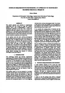
terrestrial radiation, consists of longwave, thermal infrared radiation with wavelengths from about 3,500 nm to 20,000 nm. There is little overlap between the shortwave spectrum of the Sun and the long wave spectrum of the Earth. The dominant shortwave interaction is in the UV spectral range below 300 nm where sunlight is absorbed by ozone in the middle atmosphere and never reaches the surface. Hence ozone provides an effective shield against UV radiation from the Sun. The most harmful UV radiation reaching the Earth’s surface lies in the spectral range between 280 nm and 320 nm, referred to as UV-B, while UV-A radiation at wavelengths between 320 and 400 nm is little affected by ozone (see ozone cross section in Figure 2.2a). 120

−18

10

b) 100

2

Cross Section [cm ]

a)

Altitude [km]

−20

10

−22

10

80 60 40 20

−24

10

300

400

500

600

700

0 5 10

800

10

10

15

10

20

C)

1

d)

10

Absorption coefficient

Absorption coefficient [m−1]

0

10

Density [cm −3]

Wavelength [nm]

−1

10

−2

10

−3

10

300

400

500 600 Wavelength [nm]

700

800

0.8 0.6 0.4 0.2 0

300

400

500

600

700

Wavelength [nm]

Figure 2.2 a) Absorption cross section of ozone at 261 K (Voigt et al. 2001). b) Number density of atmospheric ozone (dashed line) and total air number density (solid line). c) Absorption spectrum for pure ice (dashed line), (Grenfell and Perovich 1981; Perovich and Govoni 1991; Ackermann et al. 2006; using data from http://www.atmos.washington. edu/ice_optical_constants/, Warren and Brandt 2008), and for pure water (solid line — Smith and Baker 1981; Pope and Fry 1997; Sogandares and Fry 1997). d) Chlorophyllspecific absorption spectrum of some natural seawater normalized at 440 nm (Credit: Figure prepared by B. Hamre).

Figure 2.2b shows the number density of air, which decreases exponentially with height according to the barometric law, as well as the number density of ozone, which does not obey the barometric law because it is created and destroyed by photochemical reactions. The bulk air density determines light scattering by atmospheric molecules, while absorption is due to a variety of trace gases of which ozone and water vapor are the most important ones. For light penetration into water and ice the absorption coefficients, shown in Figure 2.2c, are needed (the optical properties of ice including scattering by ice inclusions are discussed in


•

9

Section 2.4.1). Finally, in addition to scattering and absorption by water molecules, water impurities have a large impact on light penetration. In open ocean water, the scattering and absorption properties of these impurities are often parameterized in terms of the chlorophyll concentration; the chlorophyll-specific absorption coefficient is shown in Figure 2.2d.

2.3

Clouds

Clouds have a strong nonlinear influence on the surface energy budget in the Arctic (Tsay et al. 1989; Curry and Ebert 1992; Schweiger and Key 1994; Walsh and Chapman 1998; Intrieri et al. 2002; Sandvik et al. 2007) including the timing of the onset of snowmelt (Zhang et al. 1997). The relatively thin boundary layer clouds that are prolific in spring through fall in the Arctic transmit sunlight (shortwave) and absorb thermal radiation (longwave) (Lawson et al. 2001; Intrieri et al. 2002; Zuidema et al. 2004; Lawson and Zuidema 2009). The greenhouse effect produced by this thin cloud cover accelerates melting and increases the amount of open water, which absorbs more incoming sunlight than ice surfaces, setting up a positive feedback process that leads to more melting and warming near the surface (Perovich et al. 2008; Bennartz et al. 2013). Clouds have also been observed to play a major role in sea ice loss (Kay and Gettelman 2009), but identifying the reason is a challenge because the sea ice decline over the last 30 years can be attributed to an energy surplus of just 1 W m−2 (Kwok and Untersteiner 2011). Mixed-phase clouds (MPCs), consisting of super-cooled liquid droplets and ice crystals, have been found to cover large areas in the Arctic (Shupe 2011). MPCs tend to consist of stratiform layers of super-cooled liquid water from which ice crystals form and precipitate (Curry et al. 1997; Rangno and Hobbs 2001; Shupe et al. 2006; Verlinde et al. 2007; de Boer et al. 2009; Sikand et al. 2010; Lawson et al. 2011). Even though a mixture of super-cooled droplets and ice is microphysically unstable because ice will grow at the expense of liquid water (Morrison et al. 2012), MPCs can be very persistent and often last for several days. The solar radiation field in a cloudy atmosphere is strongly influenced by scattering and absorption by cloud particles as well as by the albedo of the underlying surface.

2.3.1

Cloud optical properties

Correct treatment of the interaction of radiation with liquid water, ice, and mixed-phase clouds is important for the proper performance of climate models as well as for proper interpretation of remote sensing observations of clouds. For warm clouds consisting of spherical liquid water droplets, one may use Lorentz-Mie theory (applicable to light scattering by a dielectric sphere) to compute scattering and absorption coefficients as well as the scattering phase function for a specified size distribution of water droplets, and the known refractive index of water. Such computations require a significant amount of computing time, but fast parameterizations are available in terms of mean particle size (e.g., Hu and Stamnes 1993) which are suitable for estimating irradiances and cloud radiative forcing defined as the difference between the net irradiance in the presence of, and without, clouds.

10

•


For ice particles one must also take into account the shape of the particles, which makes the computational effort much more challenging. Thus, to quantify the radiative properties of ice clouds, in addition to the cloud particle size distribution, horizontal extent, and vertical structure, one also needs information about ice particle shape and composition (inclusions). Several investigators have attempted to parameterize the optical properties of ice clouds suitable for use in climate models (Heymsfield and Platt 1984; Sassen et al. 1995; Fu 1996; Mitchell et al. 1996a,b; Fu et al. 1998; Key et al. 2002). Despite differences in detail, existing parameterizations of ice particles in climate models have been found to yield satisfactory results for given size and shape distributions of particles (Edwards et al. 2007). To investigate the importance of particle shape, Kahnert et al. (2008) used four different non-spherical particle models to compute ice cloud optical properties and to simulate irradiances and cloud radiative forcing. They found that differences in cloud radiative forcing, downward irradiance at the surface, and absorbed irradiance in the atmosphere resulting from the use of the four different ice cloud particle models were comparable to differences in these quantities resulting from changing the surface albedo from 0.4 to 0.8, or by varying the ice water content by a factor of 2. Thus, use of a suitable non-spherical ice cloud particle model appears to be important for a realistic assessment of the radiative impact of ice clouds.

2.3.2

Cloud cover seasonality

One of the basic cloud parameters that can be derived from satellite data is the cloud fraction, which is defined as the fraction of the time that there is cloud in a certain area over a specified period. Cloud fraction is important because it provides information about the persistence and horizontal distribution of clouds that control the availability of solar energy and hence the physical and biological property and productivity of the surface. Studies of cloud fraction have been carried out using NOAA/AVHRR data (e.g., Yamonouchi et al. 1987; Schweiger and Key 1994; Wang and Key 2005). Some problems associated with the use of AVHRR data for cloud studies have been cited by Simpson and Keller (1995) and Comiso (2010). These problems include the lack of an adequate number of channels required for cloud detection, noise contamination in the 3.7 µm channel data at low temperatures, and for the polar regions, the similarity of the signatures of clouds and snow covered regions. The ability to characterize clouds improved considerably with advent of MODIS which has 36 channels, a few of which are suitable for cloud detection. Data from MODIS (and similar sensors like ENVISAT/MERIS) currently provide the most comprehensive data on cloud cover. Using MODIS data in 2007, month-to-month changes in the Arctic cloud cover fraction over sea ice and ice free oceans for the period from April to September are illustrated in Figure 2.3. This is the period when sea ice is retreating, and the Arctic region has ample sunlight and is most productive. The areas with the least cloud cover (blue) are usually located in the sea ice covered Arctic basin but the location of such areas shifts from one month to another. The ice free (open) regions near the ice edge in the Pacific and Atlantic Oceans are shown to have the highest cloud fraction (reds and oranges) with values as high as 100%. The high cloud fraction indicates a very persistent cloud cover in the open ocean even with the use of the MODIS data


•

11

Figure 2.3 Colour-coded monthly cloud fraction in the Arctic in April to September, 2007. The sea-ice extent is also presented (solid black lines).

set that is regarded as “probably clear” compared to that classified as “confident clear”. These two data sets provide very similar values over sea ice but the “probably clear” version provides significantly less and more realistic cloud cover data over ice free regions. The high cloud fraction areas in April are confined near the ice edges while medium or lower cloud fractions are observed in sea ice covered areas in the Arctic Basin, Hudson Bay and Baffin Bay, as well as the coastal areas in Europe. In May there are more clouds in the Arctic Basin and in the peripheral seas than the previous month, but not always. The retreat of sea ice in July and August is accompanied by higher cloud fractions in the Arctic Basin, especially in August when high cloud fractions are apparent even in sea ice covered areas. In September, clouds over sea ice start to recede but among the highest cloud fraction are ice free areas in the Arctic Basin. It is apparent that clouds are important factors affecting the productivity of the region. It also affects the ability to obtain consistent spatial coverage from satellite ocean colour data that are used to estimate primary productivity. The data presented is just for 2007 but similar characteristics of the cloud cover were inferred from 2010 data. The spatial distribution of clouds in the Antarctic is quite different from that of the Arctic mainly because of the large difference in the geographical location of land areas as mentioned earlier. Monthly cloud fractions in the region during the retreat of the sea ice cover from October to March 2007 are presented in Figure 2.4, where it can be seen that the seasonality is also heavily influenced by the distribution of the sea ice cover. The cloud fraction is again high in open ocean areas, but in sea ice covered regions the fractions are relatively higher than those in the Arctic. Cloud cover over sea ice increased progressively from October to

12

•


December when ice starts breaking up and retreating rapidly, with little change from January to February, when a large fraction of the ice cover has melted. It becomes less cloudy in March as the surface becomes colder and the atmosphere more dry. During the entire six month period, the ice free ocean south of 50°S is persistently cloud covered (88% – 98% cloud cover). Again, this has to be taken into consideration in the estimate of primary productivity.

Figure 2.4 Colour-coded monthly cloud fraction in the Antarctic in January to March and October to December, 2007. The sea-ice extent is also presented (solid black lines).

The MODIS cloud data provide spatially detailed information about the global cloud cover at a good temporal resolution. The cloud masking technique used to generate the standard cloud product is usually effective, but there is room for improving the accuracy of the current data set, especially in the ice free ocean regions. Through studies of concurrent A-Train observations from MODIS, CALIPSO and CloudSat, it has been shown that there are cases when the current technique is not able to identify some cloud types, especially optically thin and low clouds (Chan and Comiso 2013). The same study also shows that sometimes, areas with significant aerosol are misidentified as cloud covered areas. Improvements in the technique are thus desirable for optimal accuracy. One promising technique is a Neural Network based algorithm that makes use of CALIPSO and CloudSat data as the training data sets (Chan and Comiso, unpublished data). The technique has been shown to be effective in identifying clouds that are usually missed by the current standard technique. Another promising technique is the dynamic threshold method based on comprehensive radiative transfer simulations, which was shown by Chen et al. (2014) to be superior to the MODIS cloud mask in terms of accuracy over snow covered areas. Interannual variability and trend studies also need a longer time series than is currently available from MODIS. Improvements in the technique used for AVHRR data using enhanced MODIS data as the baseline during the period of overlapping coverage (2002 – present), would add more than three decades of satellite data that could be used for


•

13

meaningful assessments of the interannual variability and trends in polar cloud cover.

2.4 2.4.1

Ice Optical properties of the ice cover

Sea ice is a complex material consisting of an ice matrix with inclusions of liquid brine and air bubbles (Weeks and Ackley 1982). At cold temperatures, solid salts form in the brine inclusions. There may also be ice biota, sediments, and black carbon in the ice, or on the surface of the ice. This complex physical structure results in complex optical properties. Light reflection from sea ice is governed by both scattering and absorption. The spectral shape of reflected and transmitted light is determined by absorption. Figure 2.2 shows that the absorption of pure, bubble free ice has a strong wavelength dependence, with absorption coefficients ranging by more than 5 orders of magnitude (Grenfell and Perovich 1981; Perovich and Govoni 1991; Ackermann et al. 2006; Warren and Brandt 2008). E-folding lengths are more than one kilometer in the blue portion of the spectrum and only a few meters in the red. As sea ice forms, most salt is rejected from the growing ice matrix. However, some brine and air are trapped forming brine pockets and air bubbles. The large number of brine inclusions and air bubbles makes sea ice a highly scattering medium at visible and near infrared wavelengths. Because the scatterers are much larger than the wavelength, diffraction and interference can be neglected (Bohren and Huffman 1983; Grenfell 1983). Also the index of refraction of ice is a weak function of wavelength over the spectral region of interest. Thus scattering coefficients and phase functions of sea ice are often assumed to be constant with wavelength (Grenfell 1983; Light et al. 2003). Changes in the magnitude in sea ice albedo and transmittance are due to differences in scattering, with more scattering resulting in larger albedo and smaller transmittance.

2.4.2

Ice types and evolution

During initial growth, sea ice cover can form rapidly over open water (Figure 2.5a). First, the new ice consists of randomly oriented small ice grains called frazil ice that accumulate at the surface to form grease ice. This solidifies to form a thin layer of ice called nilas∗ (Figure 2.5b), which in turn becomes young ice as the ice thickens to about 15 to 30 cm (Figure 2.5c). Under quiescent growth conditions the ice growth shifts to a more orderly columnar form. In the presence of wind and waves, pancake ice (Figure 2.5d) can form. Under cold conditions (< −20°C) this entire process can occur in only a few days. Frost flowers often form on the ice surface during the initial growth phase (Perovich and Richter-Menge 1994). As the ice thickens, it is able to support a snow cover and becomes first year ice, which is the most dominant sea ice cover. There are large changes in spectral albedo during ice formation as illustrated in Figure 2.6 (Allison et al. 1993). The open water albedo is small (about 0.07) and shows little spectral ∗

Nilas: a thin, continuous elastic sheet of sea ice up to 0.1 m thick.

14

•


Figure 2.5 Photographs taken in the Arctic showing the initial growth of sea ice for (a) open water; (b) frazil ice and nilas; (c) young ice, and (d) pancake ice (Credit: D. Perovich).

variability because it is governed primarily by Fresnel reflection by the air-water interface. As the ice grows thicker, the albedo increases at all wavelengths, with the largest increases between 450 and 600 nm. The increase is due to enhanced multiple scattering in the thicker ice. More scattering results in longer pathlengths and an increased contribution from the spectral dependence of absorption. There is a large increase in albedo when an optically thick snow layer is present (red curve). Even after the initial growth phase there are still large spatial and temporal variations in sea ice surface conditions, reflectance, and albedo. Figure 2.7 shows ice surface conditions in early spring and mid-summer. In spring, the surface is a mix of snow-covered ice and open water. The contrast in albedo is extreme at visible wavelengths from 0.98 for snow to less than 0.10 for water. In mid-summer there is much more variability in surface conditions and in albedo. In addition to bare ice and open water, there is a wide variety of melt ponds. As Figure 2.7 shows, ponds range from dark (item 7) to turquoise (item 6), to light blue (item 5). Ponds are areas where melt waters collects on top of the ice, reaching depths of a few centimeters to 0.5 m (Perovich et al. 2002; Polashenski et al. 2012). The differences in pond appearance are due to the properties of the underlying ice. Dark ponds typically have thinner ice, while lighter ponds have thicker ice with more scatterers. In many cases, pond albedos decrease during the melt season as the underlying ice thins. Spectral albedos for different sea ice conditions are plotted in Figure 2.8. The highest albedos are for sea ice covered by cold, dry snow. Due to the large number of air-ice interfaces,


Figure 2.6

•

15

Spectral albedos of young growing Antarctic sea ice (after Allison et al. 1993).

Figure 2.7 Photographs showing different ice surface conditions in spring (a), and midsummer (b). Sites shown are 1) cold snow covered ice, 3) melting multi-year bare ice, 5) light blue melt pond, 6) medium blue melt pond, 7) dark melt pond, and 8) an open lead (Credit: D. Perovich).

snow is highly scattering, resulting in a large albedo. As the snow melts, scattering decreases and the albedo drops. Bare ice albedos are less than for snow, but still large (greater than 0.7) in the visible (Grenfell and Maykut 1977; Perovich et al. 2002). This is due to the presence of a surface scattering layer composed of deteriorated ice. This layer is usually a few centimeters thick. The albedo of bare melting multi-year ice is slightly greater than first year ice due to a thicker surface scattering layer and more scattering in the upper portion of the ice (Light et al. 2008). There are large differences in melt pond albedos in the visible, as discussed earlier. The light blue pond (item 5) in Figure 2.7 has a larger albedo than the other ponds, with a peak value at 470 nm (blue colour). Because of absorption in the pond water, near infrared pond

16

•


albedos are small and the same as open water (less than 0.1). 1.0

1 Dry snow 2 Melting snow 3 Melting multiyear ice 4 Melting first year 5 Light blue pond 6 Medium pond 7 Dark pond 8 Water

0.8

Albedo

0.6

0.4

0.2

0.0

400

800

1200

1600

2000

2400

Wavelength (nm)

Figure 2.8 Spectral albedos of different sea ice surface conditions in spring and midsummer. Results for 1) cold snow covered ice, 2) melting snow on sea ice, 3) melting multi-year bare ice, 4) melting first year bare ice, 5) light blue melt pond, 6) medium blue melt pond, 7) dark melt pond, and 8) an open lead. Measurements were made in the Arctic.

2.4.3

Snow on ice

Snow is highly scattering and its presence greatly increases the albedo of sea ice (Warren 1982). Figure 2.9 shows albedo as a function of snow depth for selected wavelengths in the visible and near-infrared (Perovich 2007). The results are from an experiment where new snow fell on a black base that had an albedo of about 0.15. The snow was a mix of dendrites and rounded grains roughly 1 mm in size and the density was 160 kg m−3 . There is a rapid asymptotic increase in albedo with snow depth at all wavelengths. Depending on wavelength, the snow cover was optically thick between depths of 8 to 12 cm. Snow is pervasive over both the Arctic and Antarctic sea ice for much of the year (Massom et al. 2001; Sturm et al. 2002). Observations show that from fall to summer melt, over 90% of the ice cover has an optically thick snow layer. This snow cover determines the albedo and reflectance of the surface. A key issue for Arctic sea ice is how will the ongoing shift from perennial to seasonal ice impact the snow cover. With sea ice forming later in the fall, less snow may be accumulating on seasonal ice than on perennial ice. This is a topic of current research.

2.4.4

Remote sensing of sea ice

The large scale characteristics of the global sea ice cover were not known until the advent of satellite passive microwave sensors. The robust capabilities (day/night observing, almost all weather conditions) and the large contrast of the emissivity of sea ice and that of ice free water


•

17

Figure 2.9 Impact of snow depth on albedo measured at five wavelengths. The snow fell on a black base. Measurements were made on mid-latitude snow (after Perovich, 2007).

surfaces made these sensors ideal for monitoring the sea ice cover. Continuous and consistent coverage of global sea ice cover started with the launch of Nimbus-7 Scanning Multichannel Microwave Radiometer (SMMR) which provided good data from November 1978 up to August 1987 (Gloersen et al. 1992). Nimbus-7 also carried the first ocean colour sensor called Coastal Zone Color Scanner (CZCS). The time series was continued by an operational satellite called DMSP/Special Scanning Microwave Imager (SSM/I) which has been providing continuous data from July 1987 up to the present. In the meantime, more capable systems, like the Advanced Microwave Scanning Radiometer (AMSR-E), which was launched on board Aqua of the Earth Observing System (EOS), became available. AMSR-E provided higher resolution and more accurate brightness temperature data than SMMR or SSM/I from June 2002 to October 2011 and has since been succeeded by AMSR-2 which was launched on board the JAXA/GCOM-W satellite in May 2012. Because of relatively coarse resolution (i.e., 10 – 30 km), passive microwave data have some limitations in mesoscale studies of the sea ice cover. Although the fraction of open water within each data element (pixel) can be estimated from passive microwave data, the character of the ice cover changes significantly from the ice edge into the consolidated ice pack. The character also changes with the occurrences of strong storm, polar lows and tides, and the formation of polynyas† and the Odden‡ . Some important features of the ice cover like ridges, leads, meltponds and polynyas, which have dimensions of a few meters to several meters, are difficult to study with current passive microwave systems. Several high-resolution systems are available but the coverage is not global and is usually sparse and temporally discontinuous in part because of limitations in the acquisition of highly dense data. The †

Polynya: an area of open water surrounded by ice, in a location where sea ice would be expected.

‡

Odden: a tongue of sea ice that sometimes forms during winter. It is located east of the main boundary of the

sea ice cover east of Greenland between 72 and 74° N.

18

•


preferred system for mesoscale studies has been the Synthetic Aperture Radar (SAR) which provides day/night and all weather coverage at a resolution of about 30 m. The first satellite system was the SAR on board SeaSat which was launched in July 1978, and although the satellite lasted only for 3 months, it provided insights into the great potential of the sensor for sea ice studies. Similar systems have been launched by ESA, JAXA and Canada since the 1990s and in the last decade, the technology has advanced to allow the imaging of the Earth’s surface at a resolution of 1m, as with the German System called Terra-SAR-X. Despite the high resolution, the interpretation of SAR data has not always been easy or reliable because of so many surface types. Concurrent measurements with visible and infrared systems have been used for optimum interpretation. Data from several visible systems are available, but the coverage is again sparse and, in addition, the scenes that are cloud free are difficult to find. The visible sensors that have been used most frequently are Landsat which has 7 channels and a resolution of 30 m (15m for the panchromatic) and SPOT which has even better resolution and more flexibility in the acquisition but less polar coverage. Landsat data has been available since 1972 while SPOT data started to become available in the 1980s. Cloud free data from these sensors have provided the most striking information about the distribution and spatial surface characteristics of the sea ice cover. Some studies can take advantage of MODIS 250 m resolution data in the visible which has been providing continuous global coverage since 2000.

2.4.5

Variability and trends in sea ice

2.4.5.1 Sea ice concentration, ice extent, and ice area With more than three decades of continuous passive microwave observations of the polar regions, it has become possible to make accurate assessments of the daily, seasonal and interannual variations in the sea ice cover. The basic parameter that is derived from passive microwave data is sea ice concentration, which is the percentage of the area within the field-ofview of the satellite sensor that is covered by sea ice. Several algorithms have been developed to estimate sea ice concentration and the most recent ones have been shown to provide very similar results (Comiso and Parkinson 2008; Parkinson and Comiso 2008) using AMSR-E data. The results presented in this report make use of the Bootstrap algorithm as described by Comiso and Nishio (2008). Daily ice concentration maps have been generated from passive microwave data and used to generate monthly and yearly ice concentration maps that are used to study large-scale changes in the ice cover. To illustrate how the sea ice cover has been changing on a seasonal basis, trend analysis was done on each data element of the maps using the time series ice concentration data from November 1978 to the 2012 and the results are presented in Figure 2.10a, b, c and d. The trend maps show large spatial variations in the trends in each of the four seasons with the most significant trends occurring near the ice edges. The trends are mainly negative, indicating a general retreat of the ice cover during the 34 year period with some slightly positive values in some areas, like the Bering Sea. In the winter, declines in ice cover are largest and most apparent in the Barents Sea area while in the summer, the declines are mainly concentrated in the Beaufort/Chukchi seas area. The parameters that are usually used for quantitative studies of the sea ice cover are:


•

19

Figure 2.10 Trends in ice concentration in (a) winter, (b) spring, (c) summer and (d) autumn in the Northern Hemisphere. (e) Daily averages of ice extents from January to December during the decades 1979 – 1988 (red), 1989 – 1998 (blue), and 1999 – 2008 (gold), and for each year in 2007, 2011 and 2012.

sea ice extent, which has been defined as the integral sum of ice covered areas with ice concentration of more than 15%, and sea ice area which is simply the area actually covered by sea ice estimated by taking the integral sum of the product of the area of each data element and the ice concentration estimated within the area. Ice extent thus provides information about how extensive the ice cover is and how far into the lower latitudes it may develop during each time period. Ice area provides the means to estimate the volume of the ice cover, if the average thickness of the ice is known. The sea ice cover is the most seasonal parameter on the surface of the Earth (second only to the snow cover). In the Arctic, the seasonality of the sea ice extent for different decades is illustrated in Figure 2.10e. During the first two decades of satellite data (e.g., 1979 – 1988 and 1989 – 1998), the seasonality was basically stable with the annual cycle in the ice extent changing from about 7.3 × 106 km2 in the summer to about 15.6 × 106 km2 in the winter. The ice extent was apparently about half a million km2 lower during the summer in the second decade when compared with the first, but there was very little change in the winter. During the third decade (1999 – 2008), the extent was lower than the previous decade by about a million km2 in the summer and by about half a million km2 during the winter. The average, shown in gold, includes that of 2007 (gray line) which was reported to be abnormally low in the summer (Comiso et al. 2008; Cavalieri and Parkinson 2012; Stroeve et al. 2012). Figure 2.10e also shows plots of single year data during the years when the three lowest summer minima occurred (i.e., 2007, 2011, and 2012). It is apparent that the ice extent during these 3 years was considerably lower than that of the decadal averages, with 2012 values (bold black line) even considerably lower than the 2007 values.

20

•


To evaluate the interannual changes in the ice cover quantitatively, plots of monthly anomalies of sea ice extent in the two hemispheres are presented in Figure 2.11. The monthly anomalies are derived by subtracting climatological averages (using the November 1978 to 2012 monthly data) from each month to identify monthly averages that are abnormal, and to assess trends in the ice cover. In the Northern Hemisphere, the time series shows an enhanced value in 1996 for ice extent and ice area (not shown) reflecting the abnormally high ice cover in summer of that year. This was followed by a steady decline and large interannual variability after the anomalously low summer ice cover in 2007. The large variability is caused mainly by persistently low values at the end of summer while the winter values tend to be similar to those of pre-2007 level. Trend analysis using linear regression indicates that the sea ice extent has been declining at the rate of −480, 000± 21,000 km2 (or −3.8%) per decade. For comparison, the trend in ice area (not shown) is −527, 000± 20,000 km2 (or −4.5%) per decade. The errors indicated are statistical error of the slopes of the trend line and do not reflect systematic errors that may be associated with other factors like differences in instrument calibration, resolution and incident angle between SMMR and SSM/I. The September 2012 anomaly stands out as being the most negative during the satellite era, suggesting continuation of the acceleration in the decline of the Arctic sea ice cover (Comiso et al. 2008; Parkinson and Comiso 2013). The difference in the trends in ice area compared to ice extent is, in part, due to the trend in ice concentration, which has been declining (not shown) at about −1% per decade.

Figure 2.11 Monthly ice extent anomalies in (a) Norther Hemisphere (NH) and (b) Southern Hemisphere (SH). Linear regressions are presented and the trend results (km2 per year and percentage per decade) are provided.

A surprising asymmetry in the trends of the Arctic and the Antarctic sea ice cover has been


•

21

reported (Cavalieri et al. 1997; Comiso and Nishio 2008), and it is apparent that such trend differences continue to the present. Seasonal trend maps for the Antarctic, similar to those shown for the Arctic, are presented in Figure 2.12a, b, c and d. It is apparent that the seasonal trends are predominantly more positive than those in the Arctic. In the Antarctic, the trend maps for each season also show the characteristic alternating advance and decline of sea ice along the ice edges around the continent that has been referred to as the Antarctic Circumpolar Wave by White and Peterson (1996). It is apparent that trends are strongly negative in the Bellingshausen/Amundsen Seas while they are strongly positive in the Ross Sea and other regions. This situation makes the interpretation of the trends in terms of climate change difficult, especially since the overall positive trend is caused by the larger extent of the Ross Sea ice cover than that of the Bellingshausen/Amundsen Sea. The positive trend in the extent of the Ross Sea ice cover has been observed to be mainly due to increased ice production at the coastal polynya regions (Martin et al. 2007; Comiso et al. 2011). It has been postulated through modelling studies that the ozone hole has caused a deepening of the lows in the Western Antarctic region causing stronger winds off the Ross Sea ice shelf and, therefore, more extensive coastal polynya regions and higher sea ice production (Turner et al. 2009). In the Antarctic, the sea ice cover is even more seasonal than in the Arctic with the ice extent changing from 3 × 106 km2 in the summer to almost 19 × 106 km2 in the winter. The plots of decadal sea ice cover, as depicted in Figure 2.12e, show a relatively stable Antarctic sea ice cover with the averages for the three decades almost on top of each other all year round. However, it is evident that during the 1999 to 2008 decade, the extents are slightly higher than those of the previous years.

Figure 2.12 Trends in ice concentration in (a) winter, (b) spring, (c) summer and (d) autumn in the Southern Hemisphere. (e) Daily averages of ice extent from January to December during the decades: 1979 – 1988 (red), 1989 – 1998 (blue), 1999 – 2008 (gold), and for each year in 2007, 2011 and 2012.

22

•


The corresponding plot of monthly ice extent anomalies and trends in the Antarctic is presented in Figure 2.11b. Monthly ice extent displays large interannual fluctuations with a similar number of positive and negative anomalies, and a high positive value in 2008. Despite strong negative trends in the ice cover in the Bellingshausen/Amundsen Seas, as reported previously (Jacobs and Comiso 1993; Comiso et al. 2011), the overall trend is positive (Comiso et al. 2011; Parkinson and Cavalieri 2012). The overall trend in ice extent is estimated to be 174,720 km2 /decade (or 1.5 ± 0.2%/decade) while that of area (not shown) is 207,841 km2 /decade (or 2.2 ± 0.1% per decade). The error indicated is the statistical error of the slope of the trend line as indicated earlier for the Arctic. Again, the difference in the trends for ice area and ice extent is, in part, caused by the observed positive trend (0.7%/decade) in ice concentration (not shown). 2.4.5.2 Multi-year ice and age of the ice The ice that survives the summer has been referred to as perennial ice. The ice cover during the summer minimum consists mainly of perennial ice, but because temperatures are already below freezing in parts of the ice pack during the period, there may be some contamination of new and young ice. However, the summer minimum and the perennial ice provide the same variabilities and trends, as discussed by Comiso (2002). The ice cover summer minimum has thus been used to characterize the perennial ice cover. The ice that survives at least two-summer seasons has been referred to as multi-year ice by WMO and others. This is the ice type that is retrieved from passive microwave data since it is almost free of brine and hence has the characteristic signature of fresh ice that is different from that of the saline seasonal or first year ice (Vant et al. 1978). The microwave signature of multi-year ice has also been observed to be different from that of second year ice by Tooma et al. (1975) and indirectly by Comiso (2006).

Figure 2.13 Plots of ice extents of yearly average (purple), perennial ice (blue) and multi-year ice (green) in the Arctic from 1980 to 2013.

Time series of the extent of the summer ice minimum (representing perennial ice) and


•

23

multi-year ice (as derived from passive microwave using winter data) are presented in Figure 2.13. For comparison, the yearly averages (January to December) of the extent of the Arctic ice cover are also presented. The interannual variability for the perennial and multi-year ice are shown to be coherent with each other, but that of the annual averages is significantly different. This indicates that the seasonal ice has a different interannual variability than the thicker perennial and multi-year ice cover. The overall trends are also different with the trends in extent being −3.7, −11.2, and −13.8% per decade for the yearly averages of annual ice, perennial ice and multi-year ice, respectively. This data has been updated to 2013 to show a slight recovery in 2013 from the record low in 2012. Again, the slight negative trend in the annual ice cover suggests a positive trend in the seasonal ice cover because of the much more negative trend in the thicker perennial and multi-year ice cover. The trend is mostly negative for multi-year ice indicating that the thickest component of the ice cover is the type that is declining the most. This is consistent with the observed changes in the average age of the Arctic ice cover as inferred from ice drift data by Maslanik et al. (2007) and Maslanik et al. (2011). Note that multi-year ice shows more modest recovery in 2013 and less interannual variability than perennial ice.

2.4.6

Ice thickness

Much of the past information about the basin-wide distribution and changes in the thickness of the Arctic sea ice cover has come from measurements of the ice draft by submarine upward looking sonars (Wadhams 2006). The ice draft data is converted to ice thickness assuming that the density of the ice and the thickness of the snow cover are known. Because of sparse coverage over different regions of the ice cover during different time periods, the submarine sonar data are usually difficult to interpret, especially because the sea ice cover is dynamic. Some robust data sets, however, were collected in parts of the Arctic region in the 1990s and, when compared with data during the 1958 to 1977 period, the results show significant changes in thickness as reported by Rothrock et al. (1999). In this study, the thickness in the Eurasian Basin was observed to have declined by about −1.7 m during the two periods while a decline of −0.9 m was observed in the Canadian Basin. The general decline of sea ice thickness was also reported by Wadhams and Davis (2000) in the Lincoln Sea, Fram Strait and Greenland Sea region. The results are consistent with the general decline in the thick component of the sea ice cover as reported in the previous section. Recent studies include the use of satellite measurements of the thickness of the freeboard of the ice to infer ice thickness, assuming that the density of the ice and the thickness of the snow cover are known. A study using ESA’s ERS and Envisat radar altimeter data indicates high interannual variability in ice thickness for the region south of 81°N during the period from 1993 to 2001, but no significant trends in the thickness were observed (Laxon et al. 2003). However, for the period from 2002 and 2008, a decrease of 0.25 m was observed in the Beaufort/Chukchi seas region (Giles et al. 2008) following the dramatic decline in the perennial ice cover in 2007 (Comiso et al. 2008). Studies using ICEsat lidar altimeter data from 2003 to 2008 also show thinning of about 0.6 m over areas south of 86°N covered by multi-year ice in

24

•


spring (Laxon et al. 2003; Kwok et al. 2009).

2.5

Modelled Radiation Field

The purpose of this section is to illustrate how the radiation field can be computed given the inherent optical properties discussed above of the atmosphere. The lower boundary is open ocean, bare sea ice, or sea ice covered with snow or melt ponds. Although this system is three-dimensional due to fractional cloud cover and a heterogeneous lower boundary as illustrated in Fig. 2.7, it is useful to start with a one-dimensional model and combine results with and without cloud cover, melt ponds and snow cover to mimic the behavior of the real system. Thus, for simplicity we may think of the atmosphere and underlying ocean (or sea ice with or without snow cover and melt ponds) as two vertically stratified, plane parallel, adjacent slabs with different refractive indices. To compute the radiation field in this coupled system in response to solar illumination as well as thermal emission, we must solve the radiative transfer equation (RTE): µ

dI(τ, µ, φ) dτ

=

I(τ, µ, φ) − S ∗ (τ, µ, φ) − [1 − $(τ)]B(T (τ)) Z $(τ) 2π − p(τ, µ 0 , φ0 ; µ, φ)I(τ, µ 0 , φ0 )dµ 0 . 4π 0

(2.1)

Here I(τ, µ, φ) is the diffuse radiance distribution, τ is the optical depth, µ is the cosine of the polar angle θ, φ is the azimuth angle, p(τ, µ 0 , φ0 ; µ, φ) is the scattering phase function, B(T (τ)) is the Planck function, and T is the temperature. The differential vertical optical depth is dτ(z) = −[α(τ) + σ (τ)]dz, where α(τ) is the absorption coefficient, σ (τ) is the scattering coefficient, and the minus sign indicates that τ increases in the downward direction, whereas z increases in the upward direction. $(τ) = σ (τ)/[α(τ) + σ (τ)] is the single-scattering albedo, and S ∗ (τ, µ, φ) is the source term due to attenuated solar radiation. The integro-differential RTE (Equation 2.1) can be solved using a variety of methods. For example, the discrete-ordinate method, which converts Equation 2.1 into a system of coupled ordinary differential equations, can be used to compute radiances at any desired optical depth, polar, and azimuth angle. It works as follows: (i) the upper slab (atmosphere) and the lower slab (ocean or sea ice) are separated by an interface at which the refractive index changes abruptly; (ii) each slab is divided into a sufficiently large number of homogenous horizontal layers to adequately resolve the vertical variation in the inherent optical properties (IOPs); (iii) the reflection law, Snell’s law, and Fresnel’s equations are applied at the atmosphere-ocean (or sea ice) interface; (iv) discrete-ordinate solutions to the RTE are computed separately for each layer in the two slabs; (v) finally, boundary conditions at the top of the atmosphere (TOA) and the bottom of the water are applied, in addition to continuity conditions at layer interfaces in each of the two slabs. Figure 2.14 (left) shows the simulated upward irradiance at the TOA, just above the ocean surface, and just below the ocean surface. The areas below all curves have been coloured by a


•

25

Figure 2.14 Left: Simulated upward irradiance at TOA (upper curve filled with blue colour), just above the ocean surface (middle curve filled with light blue colour), and just below the ocean surface (lower curve filled with dark blue colour). Right: Same as left panel, except that the chlorophyll concentration has been changed by a factor of 100 (After Hamre et al. 2013).

RGB translation of the spectra weighted by the three human eye colour response functions. Note the blue colour of the TOA irradiance, the light blue colour of the just above (Surface (+)) irradiance, and the dark blue colour of the just below (Surface (-)) irradiance. Figure 2.14 (right) shows results similar to those in the left panel, but for a 100-fold increase in the chlorophyll concentration. Note the significant change in sub-surface colour with increasing chlorophyll concentration, while at the same time there is only a slight change in colour at the TOA, showing that the TOA spectra are dominated by light from atmospheric scattering.

2.6

Summary

As solar radiation penetrates from the top of the atmosphere to the surface of the ice and ocean, its spectral distribution is impacted by sun angle, clouds, and ice conditions. This chapter examined the impact of these factors on downwelling and upwelling spectral irradiance. Solar radiation in the polar regions is characterized by a sparsity of sunlight in winter and an abundance of sunlight in summer. Ozone plays an essential role in providing a shield against UV exposure. Bulk air density plays a key role in light scattering by molecules. Clouds have a large impact on the surface energy budget and near-surface warming. Unusually high cloud fractions are observed from satellite data in ice free regions near the ice edge limiting the accuracy of assessing the primary productivity of these regions. The optical characteristics of sea ice are shown to vary considerably during growth stages from nilas, to young grey ice without snow cover to young ice with 2 cm snow cover and fast ice with very thick snow cover. The albedo is high and relatively stable for sea ice cover with dry snow thicker than 6 cm. The values can change dramatically during the spring and summer depending on the liquid state of the snow cover and the depth and size of melt ponds. The variabilities and trends of the sea ice cover in both hemispheres, as revealed by satellite passive microwave observations from November 1978 to December 2012, are presented. Large

26

•


interannual and seasonal fluctuations are observed but the trends are asymmetric for the two hemispheres. In the Arctic, the extent of the sea ice cover has been declining at 3.8% per decade but the ice that survives the summer (perennial ice) has been declining at a higher rate of 11% per decade. The ice that survives two summer melts (multi-year ice), which is the mainstay of the Arctic ice cover, is declining even faster at 14% per decade. On the other hand, the extent of the Antarctic sea ice cover has been increasing at around 1.8% per decade. The positive trend is mainly due to large increases in ice extent in the Ross Sea, which more than offsets the decline in extent in the Bellingshausen and Amundsen Seas. Ice production has been observed to be increasing at the coastal polynyas (which are known as ice production factories) along the Ross ice shelf, and appears to be the primary reason for the increase. Studies of ice drifts around the Antarctic appears to support this phenomenon. Sea ice data, as derived from passive microwave brightness temperature, allow for accurate identification of the ice edge even during cloudy conditions. This is important for studies of ocean colour remote sensing because it makes it possible to assess the rate of melt water production at the ice margin. Such information is required for accurate interpretation of the ocean colour distribution at the ice margin, which is expected to be influenced by the relatively stable melt water. It also allows for accurately identifying ocean colour data that is free from contamination of sea ice. Furthermore, the data can be used to keep some bona fide ocean colour data that are normally rejected because of improper evaluation of the location of sea ice. The improper masking of ocean colour data near the marginal ice zone can lead to inaccurate estimates of primary productivity in the Arctic. Radiative transfer modelling provides a means to simulate total, diffuse and direct radiance and irradiance spectra in an atmosphere-snow-ice-ocean system. The distribution of spectral radiance and irradiance is impacted by changes in the ocean chlorophyll concentration and CDOM absorption, and the TOA radiance is influenced by atmospheric aerosol loading and water constituents.

Chapter 3 From Surface to Top-of-Atmosphere Simon Bélanger, Robert Frouin, Menghua Wang, Clémence Goyens and Knut Stamnes

3.1

Introduction

The scope of this Chapter is to review in more detail the limitations of the current algorithms implemented to assess the colour of the ocean from space with respect to the particularities of polar regions. We define this part of the ocean colour processing chain as “atmospheric correction” (AC), i.e., the processing steps that aim at extracting the normalized water-leaving radiance from the top-of-atmosphere (TOA) signal, which is largely dominated by the contribution of the atmosphere between the sea surface and the satellite. In particular, we will address polar-related issues such as sea ice, low sun elevation and cloud cover. The ultimate objective of ocean colour remote sensing is to provide accurate information about the seawater constituents at synoptic scales. This goal can only be reached if the normalized water-leaving radiance (IOCCG 2010), nLw , can be estimated with high accuracy. Typically, the accuracy required for nLw at the blue bands must be 70°, which is frequent at high latitude, still needs to be assessed quantitatively and checked with actual observations. Polar Regions are also known for their persistent cloud cover (see Figures 2.3 and 2.4), especially during the late open water season when sea ice extent is minimal. Clouds can seriously reduce the amount of valid ocean colour pixels in some regions. The extent of the problem is still poorly quantified and needs more attention. In addition, clouds and ice cover can be treated together as “bright pixels” and masked out by ocean colour algorithm processing (e.g., SeaWiFS). However, one may be interested in distinguishing clouds from sea ice for several reasons, e.g., thin clouds may allow a significant amount of light to reach the sea surface, which can be harvested by phytoplankton for photosynthesis. Section 3.4 presents methods to mask clouds in current ocean colour algorithms, as well as the importance of cloud frequency for ocean colour data availability. The atmospheric composition at the South Pole, in terms of aerosols, differs substantially from the aerosol composition at the North Pole, since the South Pole is relatively isolated from continental and anthropogenic aerosols relative to the North Pole. For example, anthropogenic emissions of sulphate aerosols and black carbon from industrial cities of Northern Europe and Russia may be transported and trapped in the Arctic air mass during the polar nights of the northern hemisphere. These aerosols may significantly contribute to light scattering and absorption in the Arctic atmosphere during springtime, when the Sun rises above the horizon and creates the so-called Arctic Haze. Section 3.5.1 will review our knowledge of the polar aerosols and their implication for atmospheric correction of ocean colour images. Another important difference between the poles from the atmospheric correction perspective is the supply of particulate inorganic matter from land to sea by rivers, and coastal erosion in the Arctic coastal zones. These turbid waters are known to cause problems in AC algorithms, although schemes do exist to minimize their effect on the water radiance retrievals. Section 3.5.2 will discuss the potential zones and months where turbidity may affect the data quality in the Arctic. Approaches to detect contaminated pixels in ocean colour data are presented in Section 3.6, in presence of sea ice (Section 3.6.1) and cloud and fog (Section 3.6.2). Examples of the applications of these detection methods are shown and illustrated with MODIS-Aqua and SeaWiFS images. The last section (Section 3.7) includes a discussion about atmospheric correction schemes dealing with adjacency contamination in the presence of sea-ice and

From Surface to Top-of-Atmosphere

•

29

examples are given where ocean colour properties are derived in the presence of thin clouds and under certain conditions. Each potential problem presented above will be introduced with a literature review and illustrated with concrete examples. Methods and approaches to address these issues are presented and potential solutions discussed. In addition, new products relevant for the monitoring of high latitude marine ecosystems, such as sea ice optical properties potentially derived from ocean colour sensor information, are presented.

3.2

Issues Related to Sea Ice

Evidence of ocean colour product contamination by sea ice was first reported by Gregg and Casey (2004) in their effort to validate SeaWiFS chlorophyll data. Later, Bélanger et al. (2007) described how sea ice can introduce errors in the retrieval of chlorophyll-a and inherent optical properties (IOPs) from ocean radiance measurements. There are two ways that sea ice can contaminate ocean colour retrievals of water-leaving radiance: adjacency effects (Section 3.2.1) and sub-pixel contaminations (Section 3.2.2).

3.2.1

Adjacency contamination

Sea ice, often overlaid by snow, reflects up to 90% of the incident energy in the visible portion of the spectrum. A fraction of the photons backscattered by snow and sea ice ends up being scattered above open water pixels by air molecules and aerosols as they travel upward from the surface of the ocean up to the TOA. This process, known as the adjacency effect (Tanré et al. 1979, 1981), is defined as the change in pixel radiance caused by the atmospheric scattering of radiance that originates outside of the sensor instantaneous-field-of-view (IFOV). Formally, in the presence of adjacency effects, the reflectance at the top-of-atmosphere (ρTOA ) can be expressed according to Equation 3.1 (Tanré et al. 1979, 1981; Santer and Schmechtig 2000): ∗ ρTOA = tg (θs , θv )[ρpath + ρw + ρenv ]

(3.1)

where tg (θs , θv ) is the total gas transmittance in both downward and upward direction, ρpath ∗ is the atmospheric path reflectance, and ρw and ρenv are surface reflectance terms for the

water pixel in the presence of the adjacency effect and its environment, respectively, defined as: ∗ ρw ≈ ρw t dir (θv )

(3.2)

ρenv ≈ hρit dif (θv )

(3.3)

and

where t dir is the direct atmospheric transmittance and t dif the diffuse transmittance in the upward direction (θv ), hρi is a spatial average of each pixel reflectance over the whole surface

30

•


and ρw is the water reflectance (in absence of adjacency effect). In Equations 3.2 and 3.3, the effect of photons diffusively reflected by the water body and backscattered by the atmosphere toward the surface is neglected. In the absence of adjacency effects and sun glint, Equation 3.1 reduces to: ρTOA = tg (θs , θv )[ρpath + t(θv )ρw ]

(3.4)

where t(θv ) is the atmospheric total transmittance in the upward direction (again known as atmospheric diffuse transmittance; for details see Appendix C in IOCCG, 2010). In the presence of a non-uniform surface, however, hρi is a function of the atmospheric conditions and the mean surface reflectance, which is given by: hρi = F ρw + (1 − F )ρice

(3.5)

where ρice is the ice reflectance and F is an environmental function that represents the probability of a photon coming from space toward the target and scattered by the atmosphere to reach the surface within the IFOV. F depends on the distance between the targeted and the adjacent pixel and the atmospheric scattering properties. F is equal to unity when the ice is far enough from the target and approaches 0 when the distance between targeted and the adjacent pixel tends towards 0. Spectrally speaking, F is a function of the molecular and aerosol scattering and its spectral dependency can be expressed as: F ≈ 1/(a0 λ−1 + a1 λ−4 ),

(3.6)

where a0 and a1 are scale parameters for aerosols and molecular scattering respectively, which varies as a function of sun-viewing geometry, aerosol concentration and composition and altitude. In other words, the adjacency effect for a white surface such as snow will be small in the NIR and increases exponentially towards short wavelengths approximately following a spectral dependency of ∼ λ−4 . This results from the fact that atmospheric scattering is dominated by air molecules (Rayleigh scattering), which exhibits a λ−4 spectral dependency, and because sea ice albedo shows moderate spectral variations in the visible which drops in the near infrared (NIR) wavebands (750 to 900 nm) (Chapter 2). Potentially, it can contaminate ocean colour retrievals as far as 20 km from the ice edge (for details see Bélanger et al. 2007).

3.2.2

Sub-pixel contamination

When sea ice melts and degrades during summer, its spectral reflectance decreases progressively (See Figure 2.8 and Perovich et al. 2007) and relatively small ice floes can detach from the landfast, icebergs or the ice pack and drift in the open ocean. These pieces of ice can escape the cloud and ice detection flag, which is based on a threshold in the NIR wavebands (see Wang and Shi 2009), and be erroneously assigned by the AC algorithms as an increase in aerosols. Physically, however, the phenomenon can be compared to the effect of sea foam or whitecaps (ρwc ; Frouin et al. 1996). In such a case, Equation 3.4 can be expanded to include all surface and atmospheric contributions for a given ocean pixel:


ρTOA = tg (θs , θv )[ρR + ρa + ρRa + t(θv )[σwc ρwc − σice ρice + (1 − σwc − σice )ρw ]]

•

31

(3.7)

where ρR and ρa are the reflectance due to air molecules and aerosols alone, respectively, ρRa represents the multiple scattering interaction between molecules and aerosols; σice is the fractional sea ice coverage within the pixel (dimensionless, from 0 to 1); and σwc is the fractional coverage of whitecaps within the pixel (dimensionless, from 0 to 1). Note that the latter is always a small fraction in coarse pixel resolution (e.g., 1.1-km), even at large wind speed. Depending on the reflectance of sea ice in the NIR, σice may reach as much as 25% without being detected by the cloud and ice detection flag (e.g., thin grey ice; Bélanger et al. 2007). For example, an ice floe covered by melting snow with a ρice value of 45% at 865 nm can cover up to 6% of the surface area of a pixel before being flagged as sea ice (assuming a Rayleigh-corrected reflectance threshold of 2.7% for cloud and ice detection at 865 nm as in SeaWiFS). In terms of surface area, this represents a piece of sea ice as large as 6 600 m2 (∼80 × 80 m) in a 1.1-km pixel resolution.

3.2.3

Illustrative examples

In this section we will illustrate how ocean colour data can be contaminated by ice using several examples from SeaWiFS and MODIS-aqua data. Two different AC schemes were used to estimate the water-leaving radiance: the NASA standard AC approach (Gordon and Wang 1994; Stumpf et al. 2003) for both SeaWiFS and MODIS, and an alternative scheme proposed by Wang and Shi (2007) for MODIS that uses wavebands from the shortwave infrared domain (SWIR, 1000 – 3000 nm). For a detailed description of those AC schemes, refer to the original publications or IOCCG Report number 10 (IOCCG 2010). Briefly, the NASA standard AC algorithm, hereafter refer to as STD-AC, relies on the black pixel assumption, which assumes that all incoming radiation in the NIR (750 to 900 nm) is absorbed. Thus after removing the molecular scattering (Rayleigh) contribution to the TOA signal in the NIR, the remaining signal is assumed to come from the aerosols, which vary significantly in time and space. This approach was first proposed by Gordon and Wang (1994) and implemented successfully in the SeaWiFS processing chain in 1997. The method fails to retrieve the water-leaving radiance in the short wavebands as soon as the black pixel assumption is violated, which often occurs when there is particle backscattering, for example in turbid coastal waters or above intense phytoplankton blooms (Ruddick et al. 2000; Siegel et al. 2000). A few years later, the NASA implemented an iterative scheme to retrieve the inherent optical properties in the red bands and extrapolate these to the NIR spectral domain to assess the water reflectance in the NIR (Stumpf et al. 2003; Bailey et al. 2010). This scheme is triggered when the chlorophyll concentration, estimated from the first guess of normalized water reflectance is above 0.7 mg m−3 . The second method, hereafter refer to as NIR-SWIR, proposed by Wang and Shi (2007) is designed to deal with very turbid waters where STD-AC is expected to fail. It is based on the

32

•


assumption that the water is black in the SWIR wavebands. Those bands are only available on MODIS and were originally optimized for land applications. According to Wang and Shi (2009), the NIR-SWIR scheme can improve ice detection.

a)

c )

b)

d)

Figure 3.1 SeaWiFS standard retrievals of a) normalized water leaving reflectance at 443 nm, b) chlorophyll-a concentration from OC4v6, and total c) absorption and d) backscattering coefficients at 443 nm from a quasi-analytical algorithm (QAA). Arrows indicate evidence of contamination (very high values for nLw and bb ).

Level 1A data were obtained from the NASA Ocean Biological Processing Group and processed to Level 2 using SeaDAS 6.1. The STD and NIR-SWIR AC algorithms were applied to SeaWiFS and MODIS-Aqua data, respectively. Look-up-tables for Rayleigh and aerosol reflectance (N=80 aerosol models) for both SeaWiFS and MODIS-Aqua are those calculated by Ahmad et al. (2010). The first example is a cloud free image of the eastern Beaufort Sea captured by SeaWiFS in June 1998 (Figure 3.1). It shows the spectacular turbid plume of the Mackenzie River, the fourth-largest Arctic river, flowing into highly stratified and oligotrophic waters of the Canada Basin. Offshore in the Basin, the ice pack shows numerous leads and ice-free areas. In these waters, the retrieved normalized water-leaving reflectance in the blue (443 nm; 3.1a) reaches very high values, most likely resulting from adjacency effects. Retrieval of chlorophyll-a concentration (Chla), however, does not seem to be affected by adjacency effects since it uses spectral band ratios, which minimize the problem (Figure 3.1b).


•

33

Figure 3.2 MODIS-Aqua retrievals, after application of NIR-SWIR AC algorithm (Wang and Shi 2007), of a) remote sensing reflectance at 443 nm, b) chlorophyll-a concentration from OC4v6, and total c) absorption and d) backscattering coefficients at 443 nm from a quasi-analytical algorithm (QAA).

This holds true when the actual Chla is low, as demonstrated by Bélanger et al. (2007) (see their Figure 5), but not when Chla is > 0.5 mg m−3 . In contrast, IOP retrievals using semior quasi-analytical approaches are more sensitive to the adjacency effect as illustrated in Figure 3.1d for the total backscattering coefficient (bb ) retrieved by QAA (Lee et al. 2002). Note that the impact of the adjacency effect depends on the initial water constituents and their concentrations. At low Chla, the adjacency effect largely impacts estimates of bb as apposed to total absorption (at ). Figure 3.2 shows the same problem using MODIS-Aqua data from 29 June, 2003 in the same region. At that time, the sea ice cover was closer to the coast and adjacency contamination could be found north of the Mackenzie river plume, in the marginal ice zone. The true-colour image (not shown) indicates that the river plume was spreading below the sea ice cover. The effect of sea ice is less evident in the plume although lower Chla and total absorption coefficient (Figures 3.2b and c) were found nearby sea ice. In contrast, Figure 3.2d shows that the bb retrieval in the turbid plume is less affected by the adjacency effect (opposite to the case study described in Figure 3.1) since higher Chla is encountered. But further offshore, where Chla is lower, adjacency effects render large errors on bb retrievals (Figure 3.2d). Wang and Shi (2009) found evidence of sub-pixel contamination by sea ice in MODIS-Aqua data. Results of Wang and Shi (2009) are re-plotted in Figure 3.3. Regions with sub-pixel contamination by sea ice are circled in panels a, b, and c, showing low nLw values at 412 nm and high Chla. The effect of adjacency contamination (Figure 3.1 and 3.2) is thus opposite to

34

•


sub-pixel contamination (Figure 3.3).

Figure 3.3 An example of mixed ice-water scenario from MODIS-Aqua measurements on 26 July 2005 in the Foxe Basin around the Baffin Island, Canada for (a) true colour image, (b) nLw (412) image using the standard (NIR) AC algorithm, (c) Chla image using the standard (NIR) algorithm, (d) nLw (412) image using the NIR-SWIR AC algorithm, (e) nLw (859) image using the NIR-SWIR AC algorithm, and (f) Chla image using the NIR-SWIR AC algorithm with sea ice masking in pink (pixels masked in pink in panels (b) and (d) are for cases with nLw (412) < 0). Redrawn from Wang and Shi (2009) and reprinted with permission from IEEE.

3.3

Issues Related to Low Sun Elevation

The sun elevation at a latitude of 70°, at the satellite overpass (i.e., noon ± 1 hour), is below 20° (or sun zenith angle > 70°) for nearly six months per year. At a latitude of 80° (e.g., Svalbard) low sun elevation prevails for almost eight months per year, limiting the window for good ocean colour observations to a few summer months. Background information about the problem of low solar elevation, from a radiative transfer point of view, is provided below because the LUTs used in ocean colour processing are generated using PPA models that assume a flat Earth,


•

35

which may present a problem when the Sun is just above the horizon.

3.3.1

Theoretical background: Plane parallel versus spherical-shell atmosphere

For low sun elevations, the curvature of the atmosphere must be taken into account. In a curved atmosphere the radiance is found by solving a radiative transfer equation appropriate for spherical-shell geometry, which contains three angle derivative terms that are absent in a plane parallel (or slab) geometry (Sobolev 1975; Lenoble 1985; Dahlback and Stamnes 1991; Thomas and Stamnes 1999; Spurr et al. 2007). In a spherically symmetric atmosphere only one of these derivative terms is needed, while in spherical-shell geometry all three terms must be considered, as discussed by Thomas and Stamnes (1999). It has been shown that, in a stratified atmosphere, accurate results may be obtained for solar zenith angles less than 90° by ignoring all three angle derivatives, but using spherical geometry to compute the direct beam attenuation (Dahlback and Stamnes 1991; Slusser et al. 1996). Ding and Gordon (1994) investigated the influence of the Earth’s curvature on atmospheric correction using Monte Carlo simulations of the radiance exiting the top of a spherical-shell atmosphere. They concluded that the error in the water-leaving radiance is negligible for solar zenith angles less than about 70°. They also suggested that for solar zenith angles larger than 70°, the error in atmospheric correction can be reduced by computing the Rayleigh scattering component in spherical-shell geometry, and that the resulting error can be predicted reasonably well from computations done with a PPA radiative transfer code, in agreement with the findings of previous investigators that the ratio between the singly-scattered radiance and the total radiance is approximately the same for plane parallel and spherical geometry (Adams and Kattawar 1978; Kattawar and Adams 1978). Wang (2003) further showed Earth’s curvature effects on satellite data using real SeaWiFS measurements. To illustrate the effects of curvature on the radiation field, we show results computed by a coupled atmosphere-ocean discrete ordinate radiative transfer model (Jin and Stamnes 1994; Yan and Stamnes 2003) with a pseudo-spherical treatment of the solar beam in a curved atmosphere (Dahlback and Stamnes 1991; Spurr et al. 2007). The importance of taking curvature into account is illustrated in Figure 3.4 where (a) shows results for pseudospherical geometry at the TOA, (b) shows the corresponding results just above the water surface, (c) shows the error incurred by using the PPA at the TOA, and (d) the corresponding error just above the water surface. Computations were done for the nine MODIS ocean colour wavelengths. Denoting the radiance in upward (+) and downward (-) directions by L± (τ, µ, φ), where τ is the optical depth, µ is the cosine of the polar angle and φ the azimuthal angle, we define the TOA radiance plotted in Figure 3.4 as: LTOA (µ, φ) = L+ (τ = 0, µ, φ)

(3.8)

while the radiance emerging from the sea, i.e., the water-leaving radiance, Lw (τa− , µ, φ) = L+ (τ = τa− , µ, φ), computed as follows: Lw (τa− , µ, φ) = Locn (τ = τa− , µ, φ) − Lblack−ocn (τ = τa− , µ, φ)

(3.9)

36

•


where Locn (τa− , µ, φ) is computed for a non-black ocean, and Lblack−ocn (τa− , µ, φ) is computed for a totally absorbing (black) ocean and τa− is the optical depth from the TOA to just above the water surface. The deviation in radiance between the pseudo-spherical approximation (PSA) and the plane-parallel approximation (PPA) at the TOA is plotted in Figure 3.4c as the percentage PSA PPA difference: 100 × (LPSA TOA − LTOA )/LTOA . The use of plane parallel geometry is sufficient for solar

zenith angles smaller than about 75°, where the % difference in LTOA at 412 and 443 nm is ∼1%, whereas it is 30% for SZA > 75° (i.e., 0.1 ± 0.03 mW cm−2 sr−1 µm−1 ). Thus even a small error in the AC will have a dramatic impact on the Lw retrieval when SZA is larger than 75°.

3.3.2

Illustration of the problem

LEO satellites with a wide swath (i.e., ∼2000 km) can observe high latitudes several times per day at a time interval of ∼75 minutes. Under clear sky conditions near the solar solstice, for example, the North Water polynya, located in northern Baffin Bay (75 to 78°N latitude), can be seen by MODIS as much as seven times on the same day. Therefore, a time series of seven acquisition of the same location can be constructed to assess the reliability of ocean colour retrievals for solar zenith angles varying from ∼52° to 75°. These settings offer the opportunity to further examine the current sensitivity of ocean colour product retrievals to a gradient of SZA. Assuming that the ocean is spatially homogenous and that diurnal changes in ocean optical properties are negligible, one can expect that satellite-derived nLw and Chla will remain relatively constant over the range of SZAs explored during a given day. Table 3.1 presents the detailed sun-viewing geometry and the atmospheric parameters retrieved, namely the aerosol optical thickness (τa ) and its spectral dependency (Ångström exponent, α), for MODIS-Aqua and SeaWiFS acquisitions at three locations in the North Water Polynya (NOW) on 29 June 2004 (Figure 3.6). Note that for these cases, Ångström exponents are meaningless with such low aerosol optical thickness values, since the radiance due to aerosols is negligible in absolute terms. Huge errors in α are thus expected for such cases.

Figure 3.6 Localisation of the selected pixel to assess the impact of low sun elevation on SeaWiFS and MODIS−Aqua L2 products. The colour-coded image is the chlorophyll-a concentration retrieved by MODIS-Aqua at 16h55 UTC, 29 June 2004.

The pixel’s locations were carefully chosen to cover three Chl-a concentrations from 0.45 to ∼2 mg m−3 , and to keep sea ice typically ∼>15 km away from the chosen locations (Figure 3.6). Sky conditions during that day were particularly good for most acquisitions. Despite good and stable atmospheric conditions, cloud contamination could not be always avoided as confirmed by a careful visual inspection of each scene (not shown).


•

39

Table 3.1 Time and geometry of data acquisition on 29 June 2004 for MODIS-Aqua and SeaWiFS, for three locations in the NOW polynya. Averaged values of a 3 × 3 pixel window is taken (at the nominal spatial resolution of the sensor, i.e., 1 or 1.1-km) Sensor

Time UTC

SZA

θv

δφ

τa (865)

α

Chl

Pixel 1

74°W 55’, 77°N 30’

MODIS-A

10:25

69.1

23.5

73.3

0.027

0.57

1.76

MODIS-A

12:00

63.8

37.0

72.5

0.013

1.54

1.88

MODIS-A

13:40

59.0

33.9

71.7

0.011

1.52

2.03

MODIS-A

15:15

55.5

12.4

68.7

0.045

1.06

2.03

MODIS-A

16:55

54.1

27.3

−113.3

0.010

2.02

2.44

SeaWiFS

18:04

54.7

46.6

110.2

0.016

0.82

1.99

SeaWiFS

19:43

57.6

22.2

160.3

0.008

1.82

2.35

SeaWiFS

21:21

62.7

33

−137.1

0.010

1.67

2.23

SeaWiFS

23:00

67.4

41.4

−126.7

0.046

0.47

2.63

SeaWiFS

00:39 (+1D)

72.4

36.9

−130.7

0.005

2.14

3.21

Pixel 2

74°W 30’, 77°N

MODIS-A

12:00

63.7

40.3

73.5

0.015

1.38

0.65

MODIS-A

13:40

58.7

37.1

72.6

0.012

1.46

0.66

MODIS-A

15:15

55.0

15.5

71.5

0.016

1.00

0.68

MODIS-A

16:55

53.6

26.2

−114.4

0.011

1.80

0.67

SeaWiFS

18:04

54.3

45.7

110.8

0.009

1.56

0.58

MODIS-A

18:30

54.8

57.5

−117

0.015

1.57

0.61

SeaWiFS

19:43

57.4

21.7

169.2

0.004

1.84

0.63

SeaWiFS

21:21

62.1

35.9

−133.1

0.005

1.62

0.68

SeaWiFS

23:00

67.5

44.0

−124.6

0.002

0.36

0.98

SeaWiFS

00:39 (+1D)

72.6

39.4

−127.9

0.012

0.83

0.99

Pixel 3

76°W, 75°N 45’

MODIS-A

8:45

75.0

4.8

−106.5

0.010

−0.15

0.62

MODIS-A

10:25

69.8

34.3

73.3

0.013

0.10

0.49

MODIS-A

12:00

63.9

47.3

73.8

0.016

1.14

0.52

MODIS-A

13:40

58.3

45.2

73.2

0.024

0.97

0.52

MODIS-A

15:15

54.2

25.5

70.8

0.024

1.16

0.47

MODIS-A

16:55

52.4

18.6

-112.7

0.020

1.69

0.54

SeaWiFS

18:04

53.0

45.6

110.8

0.017

1.28

0.46

MODIS−A

18:30

53.5

55.9

−118

0.029

1.47

0.48

SeaWiFS

19:43

56.3

22.0

−178.4

0.004

2.05

0.46

SeaWiFS

21:21

61.4

41.3

-127.7

0.007

1.65

0.52

SeaWiFS

23:00

67.3

50.2

-120.7

0.007

1.86

0.57

SeaWiFS

00:39 (+1D)

72.9

46.4

-122.0

0.002

2.13

0.76

Figure 3.7 presents the nLw retrievals of MODIS-Aqua and SeaWiFS for the northern most location in a phytoplankton-rich area of the NOW polynya. SeaWiFS nLw spectra retrieved vary significantly between the first and fifth acquisition (Figure 3.7a). A general decrease in

40

•


nLw was observed along the increasing values of cos(SZA)−1 , which was more pronounced at shorter wavelengths (factor of 2 at 443 nm; Figure 3.7c). MODIS-Aqua also showed significant differences in nLw between the first and the last acquisition (Figure 3.7b), but the differences were much smaller than those for SeaWiFS (∼20% at 443 nm). Surprisingly, the relationship between nLw and cos(SZA)−1 showed an opposite trend with increasing normalized waterleaving radiance with the SZA (Figure 3.7d). Note, however, that the variations in Rrs may also reflect an actual increase in phytoplankton biomass during daytime from 10:25 UTC (1.76 mg m−3 ) to 00:39 (+ 1 day) (3.22 mg m−3 ) (Table 3.1) due to phytoplankton growth or/and advection.

Figure 3.7 Spectral remote sensing reflectance retrieved by (a) SeaWiFS and (b) MODISAqua at 77°N 30’ and 74°W 55’ in the North Water polynya, northern Baffin Bay, on June 24 2004. Variation in remote sensing reflectance at 443 and 555 nm as a function of the sun zenith angle (SZA) for both (c) SeaWiFS and (d) MODIS.

The same general trends were observed at the two locations 50 and 120 km south of the first one (Figure 3.6). However, in the clearest water located at 75°N 45’ (Pixel 3 in Table 3.1), a markedly stable nLw was observed for both sensors (not shown), even though the SZA was approaching 75°. This is above the 70° limit currently used in the L3 binning algorithm. Nevertheless, because there is a spectral dependency in the nLw differences among the acquisitions, the Chla retrieval is not constant throughout the day, but the variations were relatively small (coefficient of variation of 16%). The MODIS-Aqua Chla retrieval for the acquisition with SZA = 75° was 0.62 mg m−3 compared to 0.49 ± 0.03 mg m−3 for the six acquisitions obtained the same day. For SeaWiFS, the Chla retrieval for the acquisition with SZA = 72.9° was 0.76 mg m−3 compared to 0.52 ± 0.05 mg m−3 for the four acquisitions obtained


•

41

the same day. These results indicate that the 70° threshold for SZA used for the binning of SeaWiFS data may be appropriate or even too high, while it may be pushed beyond 70° for MODIS-Aqua. Note that for all cases, AC returns very low aerosol optical thickness, with values as low as 0.005 and even lower for SeaWiFS (Table 3.1). These values are likely too low since the atmosphere of the Arctic is known to have a non-negligible amount of aerosols (τa (500)= 0.05; Tomasi et al. 2012). This may indicate that the Rayleigh correction applied to the TOA radiance is slightly too high. On the contrary, if the effect of the Earth’s curvature was accounted for in the LUTs computation, it would tend to increase the Rayleigh contribution. This is because the Rayleigh contribution to the TOA reflectance is higher in a spherical-shell RT model relative to a plane-parallel model. Therefore, we cannot rule out a possible bias in the absolute calibration of the NIR bands of both sensors.

3.3.3

Implication of the SZA threshold on ocean colour availability

As mentioned above, it might be possible to obtain reliable estimates of nLw from MODIS-Aqua even at SZA larger than 70°, which is the current limit used in the standard L3 processing. Changing the threshold to a higher value will affect the number of potential observations in autumn, and in the northern hemisphere relative to the southern hemisphere. Here we examine the implications of using a higher threshold for SZA for the Arctic ocean. From the beginning of May to end of July, SZA is suitable for ocean colour observations in almost the entire Arctic Ocean (i.e., for latitudes from 66.68°N to 85°N; ∼13 million km2 ). Note that prior to May, the SZA is not the main factor reducing ocean colour data availability. Winter and early-spring sea ice contamination affects the usability of ocean colour images in polar seas, while low sun elevation is a factor later in the season when open water is maximum. The impact of increasing the threshold used for L3 generation from 70 to 74° was examined in terms of data coverage for the Arctic Ocean (Figure 3.8). From mid-August to mid-September the amount of data available increases significantly. For example, the current threshold limits observations to 0.5 in the Beaufort Sea, which resulted from the aerosol transported northward from the Alaskan forest fires. Time series of τa at various arctic AERONET coastal sites showed evidence of a relatively high load of stratospheric aerosols after major volcanic eruptions such as Pinatubo, Kasatochi and Sarychev that occurred in 1992, 2008 and 2009, respectively (Tomasi et al. 2012). Beyond these episodic emission events, the Arctic aerosols background concentration is lower than the global τa at 870 nm average of 0.1 (Ahmad et al. 2010). Tomasi et al. (2012) reported that 90% of the τa at 500 nm measurements fall between 0.02 to 0.08, with a mode around 0.045. In the Southern Ocean, τa rarely reaches values above 0.08, except in a period following major volcanic eruption such as Pinatubo. The composition of the aerosol determines its optical properties, which are of prime importance for atmospheric correction schemes. In general, atmospheric aerosols in polar regions are small in size yielding efficient back-scatters (Quinn et al. 2002). At Barrow, Alaska, the small fraction is mainly composed of mineral dust and sulfate aerosols while sea salt dominates the coarse fraction. In contrast, the predominant fraction of the coastal aerosols sampled in the Southern Ocean is composed of sea salt, with percentages appreciably greater than 50% and lower fractions of sulphates and mineral dust. As a result, the Arctic aerosols are slightly more absorbing than the Antarctic ones. On average, the single scattering albedo in the visible wavelengths varies around 0.95 and 0.97 for the Arctic and Antarctic aerosols, respectively (Tomasi et al. 2012 and reference therein). Spectrally speaking, the single scattering albedo tends to decrease in the NIR bands. The typical Ångström exponent is around 1 and 1.5 for the Arctic and Antarctic aerosols, respectively (Tomasi et al. 2012). In summary, these aerosol properties are not markedly different from the ones employed in the NASA standard data processing (Ahmad et al. 2010). They do not present spectral features in the visible and NIR that would invalidate the performance of the atmospheric correction in terms of water reflectance. Nevertheless, a detailed evaluation of the aerosol properties retrieved by ocean colour sensors at high latitude has never been performed. For example, several Arctic and Antarctic coastal sites are equipped with AERONET devices to monitor aerosol properties. The performance of the atmospheric correction retrieval of aerosol optical depth and Ångström exponent could be estimated. Such an evaluation could reveal important insights about the overall performance of the atmospheric correction and help to identify potential improvements.

3.5.2

Turbid waters

As outlined in the previous sections, ocean colour methods still need to be improved to provide accurate space-borne biogeochemical products over polar regions (see also Chapter 4). This is particularly true along the coastal zones where ice contribution affects the retrieved sensor-measured signal. But these coastal regions also present additional issues as they often encompass optically-complex waters, i.e., waters not dominated by phytoplankton and associated materials (also referred to as Case 2 waters, Morel and Prieur 1977). In the literature, most bio-optical models and Earth observation methods have been developed for phytoplankton


•

47

dominated waters (referred to as Case 1 waters). Indeed, waters presenting anomalous scattering in the visible and near-infrared (Case-2S for sediment-dominated; Morel and Bélanger 2006) often require more complex atmospheric correction algorithms and enhanced Earth observation methods (IOCCG 2000, 2010).

Figure 3.13 Visualization of the Case-2S waters in the Arctic by applying Lee and Hu (2006) criterion to MODIS-Aqua monthly climatology composite distributed by the NASAOBPG. Results are shown as the percentage relative difference between the actual Rrs (555) value and Rrs (555)LIM (see text). Red pixels can be considered as Case-2S waters.

Figure 3.13 shows the presence of Case-2S waters in the Arctic Ocean from May to August based on the climatology of MODIS-Aqua data. Case-2S waters are identified here based on an inclusive Case-1 remote sensing criterion developed by Lee and Hu (2006). The criterion compares the actual Rrs (555) with an expected Rrs (555) value estimated according to a Case 1 bio-optical model (denoted as Rrs (555)CASE1 ) including a spectral reflectance ratio at 555 and 490 nm (Morel and Maritorena 2001). Hence, any pixel showing a Rrs (555) value that deviates by more than 50% from the estimated Rrs (555)CASE1 is considered to present anomalous scattering in the visible. As suggested by Lee and Hu (2006), a 50% deviation is used since only a limited number of natural waters follow the quantitative relationships for Case-1 waters. Rrs (555)LIM

48

•


is therefore defined as 1.5 times Rrs (555)CASE1 . According to Figure 3.13, which shows the percentage relative difference between the actual Rrs (555) value and Rrs (555)LIM , Case-2S waters are mostly encountered in Foxe Basin, along the coast of the Beaufort Sea, along the west-coast of Alaska in the Bering Sea and in the East Siberian Sea, from May to August. Most of these regions are indeed affected by river inputs as well as coastal erosion, resulting in a significant supply of organic matter from coastal land. Figure 3.13 also shows that the presence of Case-2S waters increases from May to August. Indeed, ice-melt and glacial run-off from nearby land also represents a large input in sediment loading. With the ongoing climate change, ice melt and polar precipitation are expected to increase, leading to increased coastal turbidity. In July and August a large patch of anomalous scattering in the visible is also noticeable in the Barents Sea. This patch of Case-2S waters results from coccolithophore blooms, known to occur in late summer in this region (e.g., Smyth et al. 2004). As demonstrated earlier by Bélanger et al. (2007), in polar regions, turbid pixels are often erroneously identified as sea-ice contaminated pixels due to adjacency effects. Figure 3.13 confirms this plausible confusion between ice contamination and turbid coastal waters. Indeed, speckle patterns of anomalous scattering are observable in the Beaufort Sea, on the Mackenzie Shelf, and in the East Siberian Sea, mostly in May and June. These speckle patterns may result from ice-contamination due to the presence of floating ice sheets. Note, however, that at this time of the year an increase in particulate organic matter (POM) is also expected nearby ice-floes due to multi-year ice melting, but this should not increase Rrs (555) due to the highly absorbing nature of POM (Bélanger et al. 2013a; their Figure 9b). Hence, in polar regions, Earth observation methods should consider the spectral properties of optically-complex waters, in addition to the multiple and divergent spectral impacts of sea-ice.

3.6 3.6.1

Detection of Contaminated Data Detection of adjacency effect and sub-pixel contamination

Bélanger et al. (2007) proposed a simple method to identify pixels contaminated by the adjacency effect, based on examining the spectral shape of the water-leaving reflectance in the violet-blue wavebands, which are the most affected by adjacency effects. The normalized water reflectance band ratio between 412 and 443 [Rrs (412)/Rrs (443)] tends to increase with increasing adjacency effect with values typically above 1. In contrast, the remote sensing reflectance spectra in polar regions tend to present values of [Rrs (412)/Rrs (443)] below 1, because of a higher background in CDOM in those regions (Reynolds et al. 2001; Wang and Cota 2003). The Rrs (412)/Rrs (443) threshold above which pixels are contaminated by adjacency effects can be adjusted as a function of the reflectance in the green following the relationship: Threshold = C − 0.14 log10 π ∗ Rrs (555) ,

(3.11)

where C is an offset that requires tuning, depending on the region. A value of 0.64 for C was found acceptable for the Beaufort Sea (Bélanger et al. 2007). This threshold is sensitive to the


•

49

CDOM concentration, because of the use of the shortest wavebands, and is expected to vary from region to region. Wang and Shi (2009) also proposed a method to detect ice and sub-pixel contamination when the NIR-SWIR scheme is used to process MODIS data. With this atmospheric correction scheme, cloud masking is made using the 1240-nm channel rather than the typical 865-nm channel (Wang and Shi 2006). While the NIR-based cloud masking can remove most sea ice contaminated pixels, the SWIR-based cloud masking skips several ice-contaminated pixels. This is because sea ice has a rather low reflectance in the SWIR compared with NIR bands (Figure 2.8). Consequently, Wang and Shi (2009) proposed a method to detect ice-contaminated pixels based on the excess of radiance in the NIR bands that resulted after the application of NIR-SWIR atmospheric correction algorithm. In theory, this method will not detect adjacency contamination because the process does not substantially affect NIR wavebands. For polar regions (latitude >55°), it was proposed that pixels with nLw (859) > 0.2 mW cm−2 µm−1 sr−1 are masked (see Wang and Shi (2009) for details). Examples of the application of these methods are shown in Figures 3.14 and 3.15 using MODIS-Aqua data. Note that the adjacency methods can be applied to any ocean colour sensor, while the ice detection method of Wang and Shi (2009) is suitable only when SWIR bands are used in the data processing. The adjacency flag proposed by Bélanger et al. (2007) performs very well in the Beaufort Sea (Figure 3.14a) as most pixels in the proximity of large sea ice patches are identified. For the same image, the Wang and Shi (2009) flag was raised over the Mackenzie River plume because of the water turbidity (Figure 3.14b), and was also raised in an area where an ice floe is detached from the landfast ice (see Figure 3.14d-e). A closer examination of the MODIS 250-m NIR band confirmed that pixels flagged in this area were affected by undetected small pieces of sea ice (Figure 3.14e). The contaminated pixels found in the ice floe showed slightly higher values of aerosol optical thickness (∼0.05 versus 0.02 for the surrounding pixels), but the chlorophyll retrieval did not present evidence of severe contamination when compared to adjacent pixels (not shown). In terms of IOP retrievals, however, undetected sub-pixel contamination has a serious impact on data quality. The Wang and Shi (2009) method may misinterpret ice-contaminated and turbid waters pixels (Figure 3.14b), because non-negligible nLw (NIR) is generally found for the latter. At latitudes lower than 55°, Wang and Shi (2009) proposed a second spectral test to distinguish turbid and ice-contaminated pixels using a band ratio (Rrs (555)/Rrs (412)), but this approach failed when sub-pixel contamination produced an underestimation of the reflectance at 412 nm. Sea ice contamination flagging was tested in two other sectors: in Baffin Bay (Arctic) and in the Ross Sea (Antarctica). A MODIS-Aqua image of Baffin Bay during the ice edge bloom observed in June 2007 was chosen (Figure 3.15a–d). Perrette et al. (2011) described this particular phytoplankton bloom using SeaWiFS imagery (their Figure 3). The use of the MODIS-Aqua 250-m channels was helpful to detect whether potential sub-pixel contamination by sea ice could explain the bloom. According to the sub-pixel contamination flag of Wang and Shi (2009), only a few pixels were affected by small pieces of sea ice (Figure 3.15d). Examination of the 250-nm channel did not show evidence of extensive contamination within the high

50

•


Figure 3.14 Examples of the application of ice-contamination flagging methods (pink) proposed by a) and c) Bélanger et al. (2007) for adjacency contamination (with C = 0.7 in Equation 3.11), and b) and d) Wang and Shi (2009) for ice and ice mixed pixels. The black square in panel b) is magnified in c) and d), and that in panel d) is magnified in panel e). Images a) – d) show Rrs (443) while image e) shows the surface reflectance of the MODIS 865 nm channel (250-m resolution) which allows a better appreciation of the broken ice field.

chlorophyll patch detected by MODIS (not shown), suggesting that ice edge blooms are not an artifact of ocean colour algorithms. In contrast, relatively low Chla was observed along the ice edge as a result of the adjacency effect (Figure 3.15b), which artificially increases the blue-to-green water reflectance ratio. The adjacency flag (Figure 3.15c), however, masked out a very large band, up to ∼50 km from the ice edge, comprising the bloom itself. This result is incompatible with the simulations performed by Bélanger et al. (2007) which suggested that adjacency effect should not be important >20-km away from the ice edge. The thresholds determined by Bélanger et al. (2007) (Equation 3.11) for the Beaufort Sea are not adapted for optically-different water masses, since the Rrs (412)/Rrs (443) ratio depends on the magnitude of CDOM absorption, which is much higher in the Beaufort Sea relative to other polar regions. CDOM absorption in the Ross Sea is much lower (Chapter 4), making the reflectance ratio at 412 and 443 nm higher than that of the Beaufort Sea. Consequently, all pixels in the Ross Sea were flagged (Figure 3.15g) with the method. These results indicate that a regional tuning of the adjacency flag threshold is necessary for application of this method at large scale. In summary, sea ice contamination flagging is possible but the methods are not ready for implementation in the operational processing of ocean colour data. Future work should aim at generalizing the approaches, and exploring other strategies to avoid contamination of high-latitude ocean colour products.


•

51

Figure 3.15 Sea ice contamination flagging of on an ice edge bloom in Baffin Bay (MODISAqua scenes a–d) and (e) Ross Sea, Antarctica (SeaWiFS). a) MODIS-Aqua quasi true-colour image; b) Chla derived from OC3 algorithm; c) Bélanger et al. (2007) flag; d) Wang and Shi (2009) flag; e) SeaWiFS quasi true-colour image of the Ross Sea; f) Chla derived from OC4 algorithm; g) Bélanger et al. (2007) flag. Note that the Wang and Shi (2009) flag is not applicable on SeaWiFS as it requires SWIR bands.

3.6.2

Cloud detection in ocean colour algorithms

Ocean colour remote sensing is only possible over oceans with a clear atmosphere (cloud-free), requiring cloud-masking for standard ocean colour data processing (Ackerman et al. 1998). For SeaWiFS and MODIS, Rayleigh-corrected NIR reflectance threshold at 865 nm (869 nm for MODIS) is used to identify clear sky pixels for processing of ocean colour products (Robinson et al. 2003). Specifically, the standard SeaWiFS/MODIS cloud-masking uses the NIR Rayleigh-corrected reflectance threshold (δρ (RC) (NIR)) computed as δρ (RC) (NIR) = ρTOA (NIR) –ρR (NIR), where

52

•


ρTOA (NIR) and ρR (NIR) are the sensor-measured reflectance and the Rayleigh scattering reflectance from lookup tables, respectively (Gordon et al. 1988a; Wang 2002, 2005). Over open oceans, the NIR ocean radiance contribution is usually negligible (i.e., the black ocean assumption). Thus, the Rayleigh-corrected TOA reflectance results predominantly from aerosol reflectance contributions for clear atmosphere. A threshold value of 2.7% in δρ (RC) (NIR) is used for the cloud masking, which corresponds to an aerosol optical thickness of ∼0.3 in the NIR for maritime aerosols (Wang and Shi 2006). The SeaWiFS/MODIS cloud-masking scheme usually performs well over the global open oceans, because the ocean is usually black at the NIR band, and aerosols are generally dominated by maritime aerosols (Smirnov et al. 2002; Knobelspiesse et al. 2004; Wang et al. 2005b). SeaWiFS and MODIS have provided high quality ocean colour products over the global open oceans (McClain 2009), although significant errors in cloud-masking could have occurred in the coastal regions when using the NIR threshold scheme due to ocean contributions in the NIR spectral domain and aerosol reflectance from non-maritime aerosols (e.g., aerosols with small particle size from pollution, Wang and Shi 2006). Subsequently, cloud masking using the SWIR bands has significantly improved performance over coastal turbid waters (Wang and Shi 2006). Corresponding to the Rayleigh-corrected reflectance threshold of 2.7% at the NIR, the reflectance thresholds for the SWIR 1240, 1640, and 2130 nm bands are 2.35%, 2.15%, and 1.75%, respectively. For sensors without SWIR bands (e.g., SeaWiFS), cloud detection has been improved by using the Rayleigh-corrected reflectance ratio value from two NIR bands in addition to the reflectance threshold at 865 nm. This is simply because clouds are generally spectrally flat and have lower NIR reflectance ratio values relative to ocean and aerosols (Wang and Shi 2006). In polar regions, however, cloud detection over sea ice is challenging. The SeaWiFS/MODIS cloud-masking scheme may not distinguish clouds from sea ice, since both increase the NIR reflectance beyond the threshold. Note, however, that MODIS Cloud Products (MYD35) are obtained using a combination of several bands including visible, NIR and thermal IR bands. Moreover, the MODIS cloud mask algorithm uses several cloud detection tests allowing the estimation of a confidence level for clear-sky scenes. The MODIS cloud mask algorithm employs up to 14 MODIS spectral bands to maximize reliable cloud detection (Ackerman et al. 1998). Despite significant improvements (Frey et al. 2008), MODIS cloud detection is still negatively biased over sea ice (Liu et al. 2010). A comparison of the MODIS cloud mask product with the Cloud-Aerosol Lidar and Infrared Pathfinder (CALIPSO) indicated a better performance of the algorithm over open water in the Arctic (Liu et al. 2010).

3.7

New approaches for processing ocean colour data and new geophysical products

3.7.1

Advances towards solving the sea-ice and cloud contamination problem

Adjacency effects may be important when viewing the ocean in the presence of snow/ice (Section 3.2). They can be detected using the spectral shape of the retrieved water reflectance


•

53

(Section 3.6), or they may also be corrected. This can be accomplished by first applying the selected atmospheric correction scheme ignoring adjacency effects (i.e., assuming that the target is infinitely large). The retrieved water reflectance and aerosol properties can then be used to estimate the environment reflectance and the atmospheric functions Ta and td , therefore ρenv . In the next step, ρenv is subtracted from ρTOA /tg , and the selected atmospheric correction scheme is applied again. This gives a second estimate of ρwN . After some iterations, a final ρwN is obtained, corrected for adjacency effects. The advantage of correcting the ocean colour imagery for adjacency effects, as opposed to detecting its presence, is that the contaminated pixels are not discarded, i.e., spatial coverage of the water reflectance and derived products are not compromised. Computing the environment reflectance is, however, computer intensive, since it requires convolving the spatial ρw field with the atmospheric spread function over a distance of at least 10 km (the typical horizontal scale of the adjacency effect due to molecular scattering). Furthermore, the atmospheric spread function is critically dependent on the altitude (or scale height) of the aerosols, a parameter not routinely estimated from space. Nevertheless significant improvement in ρw retrieval is expected using a typical aerosol profile (e.g., from climatology or an atmospheric transport model). Note that this approach is also applicable to ocean pixels in the vicinity of clouds. Like snow/ice, clouds may scatter unwanted light in the instrument field-of-view. Correcting for this light may contribute to higher quality ocean colour products and larger spatial coverage, a desirable outcome in the Arctic Ocean which is strongly affected by cloud cover (see Section 3.4). In the absence of information about cloud altitude, the correction may assume, in first approximation, that clouds are located at the surface. Another approach to correct for adjacency effects due to snow/ice and clouds is based on the observation that the perturbing signal from the atmosphere and surface, i.e., ρpath + ρenv in Equation 3.1, varies smoothly with wavelength and can thus be approximated by a polynomial with a few terms. This is the principle of the POLYMER algorithm proposed by Steinmetz et al. (2011), originally developed to process MERIS imagery in glitter-affected areas. The algorithm fits ρpath + ρenv by a polynomial with (1) a non-spectral term that accounts for any non-spectral scattering (clouds, coarse aerosol mode) or reflection (glitter, whitecaps, small ice surfaces), (2) a spectral term with a power law in λ−1 (fine aerosol mode), and (3) a spectral term with a power law in λ−4 (molecular scattering, adjacency effects from clouds and white surfaces). We recall here that the coupling between molecular scattering (spectral effect in λ−4 ) and diffuse reflection by a white surface (no spectral effect) varies like λ−4 λ0 = λ−4 . No aerosol model is used, giving simplicity and robustness to the algorithm. Figure 3.16 displays an example of processing in the Beaufort Sea, at the delta of the Mackenzie River. In the top left part of the image, open waters are surrounded by ice floes. The POLYMER processing (middle right, and bottom right) retrieves a consistent marine reflectance at 560 nm over ice-free areas in the middle of the ice pack. The standard MEGS processing, on the other hand, does not account for environment effects (middle left and bottom left), leading to an anomalous increase of water reflectance. This is explained by a too low spectral dependence of the atmospheric signal estimated from spectral bands in the near infrared. Indeed, in this part of the spectral domain, molecular scattering, and subsequently ice reflection

54

•


from adjacent sea-ice is relatively ineffective.

Figure 3.16 MERIS image of the Beaufort Sea (4 July 2008), showing that the marine reflectance at 560 nm derived by the POLYMER algorithm is consistent over ice-free areas in the middle of the ice pack, while the MEGS processing is affected by the ice environment, leading to an anomalous marine reflectance increase. (Courtesy of F. Steinmetz, HYGEOS.)

The POLYMER algorithm is also able to handle situations of thin clouds, which makes it especially useful to increase spatial coverage of ocean colour products. The polynomial approximation for the perturbing signal is still valid in such situations, and the effect of cloud transmittance on the water reflectance, not accounted for in the algorithm, is compensated by the effect of the backscattering coefficient for non-phytoplankton particles, one of the


•

55

parameters used to minimize the difference between modelled and observed TOA reflectance (for algorithm details, see Steinmetz et al. 2011). Figure 3.17 gives an example of results obtained with MERIS imagery of the Chukchi Sea in the presence of a large semi-transparent cloud. The POLYMER algorithm retrieves marine reflectance in all the thin cloud areas masked by the MEGS algorithm, and the marine reflectance features under the clouds exhibit continuity with those of the adjacent, cloud-free areas. Note that other atmospheric correction algorithms, which also use all available spectral bands for atmospheric correction, have the potential to deal effectively with thin clouds. In the statistical methodology of Gross-Colzy et al. (2007a,b) in particular, large aerosols with optical properties that resemble those of cloud droplets are considered. Therefore, cases of thin clouds are virtually represented in the principal component analysis of the TOA signal, leading to accurate mapping of the useful components to the marine reflectance (for algorithm details and examples of application in the presence of clouds, see Gross-Colzy et al. 2007a,b). Performance in cloudy conditions with this type of algorithms is expected to improve by specifically taking into account realistic cloud cases in the ensemble of simulated TOA reflectance.

3.7.2

Retrieval of sea ice optical properties using ocean colour data

Recent observations of phytoplankton blooms under sea ice (Mundy et al. 2009; Arrigo et al. 2012) has led to a growing interest for remote sensing of sea ice optical properties. In addition, coupled sea ice-atmosphere-ocean-biogeochemical numerical models have predicted significant primary production under sea ice in the future Arctic Ocean (Popova et al. 2010). Light transmission across sea-ice depends on its optical properties, the presence of snow cover and melt ponds etc. (see Chapter 2). The presence of melt ponds, for example, indicates major increase in light transmission through sea ice, significantly impacting the biological activity underneath. Optical sensors used in ocean colour remote sensing may be used, potentially, to derive some optical properties of sea ice. Until recently, most of the sea ice optical observations have been made in situ. Even though in situ studies can provide details on sea ice physical and optical properties, they have some limitations. Collecting in situ sea ice data at high latitudes is both labor-intensive and timeconsuming, and often confined to a relatively short time period. The lack of spatial coverage and long-term observations makes it impossible to study the impact of the sea ice on climate and ecosystems at a large scale. In contrast, satellite remote sensing can provide synoptic views of global land, ocean, and atmosphere. Even though a variety of satellite sensors can provide global sea ice information, such as passive microwave sea ice concentration from the Advanced Microwave Scanning Radiometer EOS (AMSR-E, Cavalieri and Comiso 2000; Comiso et al. 2003), MODIS sea ice extent data (Riggs et al. 1999, 2006), and ice sheet elevation data from the Ice, Cloud, and land Elevation Satellite (ICESat, Kwok et al. 2004; Schutz et al. 2005), no sea ice reflectance data have ever been retrieved for the global ocean in the visible and NIR bands with MODIS observations. Shi and Wang (2012a,b) demonstrated that sea ice reflectance spectra at MODIS-Aqua visible and NIR wavelengths can be derived reasonably accurately in the Bohai Sea after carrying out

56

•


Figure 3.17 MERIS image of the Chukchi Sea (21 August 2007) showing that water reflectance in the presence of a large semi-transparent cloud is retrieved in some cloudy areas by the POLYMER algorithm (top right), but not by the MEGS algorithm (top left). (Courtesy of F. Steinmetz, HYGEOS.)

atmospheric correction using the MODIS SWIR measurements at the 1640 and 2130 nm bands. In situ sea ice spectral albedo measurements in the polar regions show that the spectral albedo values drop sharply from the NIR to SWIR wavelengths for all types of sea ice (Heymsfield and Platt 1984; Perovich 1996). For the MODIS SWIR wavelengths at 1640 and 2130 nm, the sea ice reflectance values are small (normally less than ∼0.05), compared with ice reflectance in the visible wavelengths (that can reach ∼0.9) for both snow-covered and other types of ice in the polar regions (Perovich 1996). Thus, MODIS SWIR bands at 1640 and 2130 nm can be used for atmospheric correction for deriving sea ice optical properties (Shi and Wang 2012b). A MODIS-Aqua-measured true colour image on 12 February 2010 in the Bohai Sea, on which sea ice coverage is clearly visible, has been corrected for atmospheric contribution using


•

57

the MODIS-Aqua bands at 1640 and 2130 nm (Wang 2007). The reflectance values over both the ocean and sea ice (the green-yellow colour on Figure 3.18) are derived at different MODIS wavelengths. Figure 3.18 shows the normalized water-leaving reflectance maps of the entire Bohai Sea at 412, 443, 555, 645, 859 and 1240 nm. Significant contrast can be identified between the ocean water and sea ice coverage for all the wavelengths except 1240 nm. For the ocean water region, normalized water-leaving reflectance ρwN (λ) spectrum is featured with peak values at ∼0.15 for 555 and 645 nm bands (Figure 3.19). At 443 and 859 nm, however, ρwN (λ) values are generally weak. At the SWIR 1240 nm band, the normalized water-leaving reflectance is close to zero. For the sea-ice-covered region, reflectance values are significantly enhanced for all the visible and NIR wavelengths. Peak reflectance values over the sea ice region occur at wavelengths of 555 and 645 nm. Sea ice reflectances at these two wavelengths reach over ∼0.30 for a large part of the sea-ice covered area in the Bohai Sea.

Figure 3.18 Normalized water-leaving reflectance at (a) 412 nm, (b) 443 nm, (c) 555 nm, (d) 645 nm, (e) 859 nm, and (f) 1240 nm derived from MODIS-Aqua measurements on 12 February 2010 using the SWIR atmospheric correction algorithm with the band set of 1640 and 2130 nm. Note that the colour scale for (f) is different from others and is indicated in the panel (from Shi and Wang 2012a).

Figure 3.19 further quantifies the normalized water-leaving reflectance values for different ocean surface types, i.e., coastal turbid waters, central Bohai Sea waters, dark and light ice, grey ice, and grey-white ice. However, it is noted that the properties of sea ice in the polar region are different from those in the Bohai Sea, e.g., the SWIR sea ice albedo in the Polar Region is still significant. Thus, it is still a challenge for deriving accurate sea ice optical property data from ocean colour satellite sensors in the Polar Regions.

58

•


Figure 3.19 Comparison of the satellite-derived normalized water-leaving reflectance spectra on 12 February 2010 for coastal turbid waters at 38.21°N, 119.09°E (location C in Figure 3.18f), central Bohai Sea waters at 39.04°N, 119.62°E (location D in Figure 3.18f), grey ice at 39.89°N, 120.96°E (location E in Figure 3.18f), grey white ice at 40.10°N, 121.36°E (location F in Figure 3.18f), and dark ice at 40.71°N, 121.67°E (location G in Figure 3.18f) (from Shi and Wang 2012a).

3.8

Recommendations

Several conclusions and recommendations can be drawn from this review, the most important of which is the need to assess the overall accuracy of the normalized water-leaving radiance and atmospheric retrievals distributed by the space agencies. In this report, we have shown clear evidence of contamination of the signal by sea ice, but the extent of the problem and how it is reflected in higher level data products (e.g., Level 3) remains to be demonstrated.

v Considering the importance of marginal ice zones (MIZ) in terms of ocean biology and primary production in both poles (Comiso et al. 1990; Perrette et al. 2011), the problem of sea ice contamination needs more attention and new approaches to improve the data coverage and the data quality need to be developed, tested and validated. Data fusion between moderate (300 – 1000 m) and high resolution (10 – 30 m) satellite sensors in the MIZ may be possible with recent and future missions such as Landsat-8, VIIRS, Sentinel-2 and -3, and PACE.

v Low sun elevation strongly limits data coverage in late summer and autumn. Based on radiative transfer calculations and a limited dataset, it may be possible to extract ocean optical properties at solar zenith angles beyond the 70° threshold adopted by space agencies. Before extending the threshold, however, more work is needed to ensure the data quality is not being degraded for the benefit of data coverage.

v Multiple satellite overpasses at high latitudes provide several observations of the same location during clear sky days. These multiple observations offer opportunities to study the SZA problem as well as short-term oceanographic features (e.g., surface currents, phytoplankton growth rates, export production). It also brings into question the method used to aggregate multiple overpasses when producing Level 3 data (e.g., should all observations on a given day be averaged, or only those nearest to noontime?)

v Considering the prevalence of clouds at high latitudes, there may be some data gaps.


•

59

Gap filling methods are required when biogeochemical fluxes are estimated from ocean colour data (e.g., primary production, see Chapter 5). This problem needs to be examined in depth, and fusion with in situ autonomous systems may be explored in the near future.

v Aerosol retrievals in polar regions need to be examined to obtain new insights in the performance of atmospheric correction algorithms. Weekly and monthly values may be substantially biased.

v Turbid waters occupy a significant fraction of many coastal arctic regions. Although common to all coastal regions, this problem will need to be considered for long-term monitoring of polar ecosystems.

60

•


Chapter 4 Ocean Colour Algorithms and Bio-optical Relationships for Polar Seas Rick A. Reynolds, Atsushi Matsuoka, Toru Hirawake, Simon Bélanger, and B. Greg Mitchell

4.1

Introduction

In this chapter, the performance of existing ocean colour algorithms for estimating the concentration of chlorophyll-a (Chla) in surface waters is assessed when applied to polar oceans and their marginal seas. The discussion is limited to relationships within or immediately above the sea surface, omitting additional challenges to satellite retrievals which arise from low sun angle, atmospheric conditions, and the presence of sea ice. We first examine application of standard empirical algorithms commonly employed for global use, which are based on relationships derived from large oceanic datasets in which polar regions are typically underrepresented. We then explore differentiation in underlying bio-optical relationships for polar seas and discuss their potential influence on empirical algorithms. A simplified sensitivity analysis using semi-analytical modelling is used to show that differing bio-optical relationships can explain the observed deviations from empirical algorithms formulated for non-polar waters. There have been reports in the literature for several years that the relationships between ocean colour and Chla in polar regions differ markedly from lower latitude waters. A multitude of studies (Mitchell and Holm-Hansen 1991; Mitchell 1992; Arrigo et al. 1998; Dierssen and Smith 2000; Hirawake et al. 2000; Reynolds et al. 2001; Korb et al. 2004; Garcia et al. 2005; Mitchell and Kahru 2009) have indicated that standard ocean colour algorithms perform poorly when applied to waters of the Southern Ocean. Similar observations have been noted in the Arctic Ocean and northern polar seas (Mitchell 1992; Sathyendranath et al. 2001; Cota et al. 2003; Wang and Cota 2003; Stramska et al. 2003; Cota et al. 2004; Matsuoka et al. 2007; Naik et al. 2010; Ben Mustapha et al. 2012). The differences are often explained by the adaptation or acclimation of polar phytoplankton to extreme environmental characteristics such as low solar radiation and cold temperature, or because of alterations in the relative abundances and characteristics of other optically-significant constituents resulting from particular geographical settings. These individual studies are based on limited data collected in specific regions, which hinders the extrapolation of the findings to widespread areas. 61

62

•


A further complication arises in that methods for measuring Chla have evolved over time, with different techniques employed by various studies. The fluorometric method, which estimates chlorophyll-a concentration from measurements of stimulated fluorescence by chlorophyll molecules extracted in solvent, has a long tradition in oceanography and has been employed extensively in past studies. It is a relatively simple and inexpensive measurement, but can be subject to inaccuracies caused by the concomitant fluorescence of other pigments present in solution. In modern times, these problems have been circumvented by the development of more advanced techniques such as High-Performance Liquid Chromatography (HPLC) which enable the separation and quantification of individual pigments with much greater accuracy, at the cost of higher analytical complexity and expense. The two measurements are generally highly-correlated, but may exhibit significant offsets relative to one another in some marine environments (Trees et al. 1986; Neveux et al. 1990). This confounds the interpretation of historical results for polar regions, in which the fluorometric method was predominantly used. Ultimately, systematic deviations from the empirical models observed in polar waters imply differences in the underlying bio-optical relationships. The inherent optical properties (IOPs) of seawater, which are dependent solely on the medium and independent of the directional structure of the light field, strongly influence the magnitude and spectral shape of the light field emerging from the ocean. These quantities include the spectral absorption coefficient, a(λ), and the volume scattering function, β(Ψ , λ), with the latter describing the radiant intensity of light at wavelength λ scattered by a unit volume of water at an angle Ψ per unit irradiance of the incident light beam (see Mobley 1994 for a review of definitions and notation in hydrologic optics). Integration of the volume scattering function over the backward hemisphere yields the spectral backscattering coefficient, bb (λ), which is of fundamental importance to optical remote sensing. To a first approximation, the spectral remote-sensing reflectance, Rrs (λ), is directly proportional to the backscattering coefficient and inversely proportional to the absorption coefficient through the relationship (Gordon et al. 1988b; IOCCG 2006):

Rrs ≈ C(λ)

bb (λ) , a(λ) + bb (λ)

(4.1)

where C is a proportionality factor which merges several directional aspects of radiative transfer and the transfer of light across the sea surface. The IOPs in turn are directly related to the concentrations and optical properties of water molecules, dissolved substances, and particles — thus providing an important linkage between remote-sensing reflectance and the concentration and relative proportions of seawater constituents. For a seawater suspension containing suspended particles and dissolved materials, both the absorption and backscattering coefficients of the suspension can be viewed as the cumulative sum of the partial contributions by each optically-significant constituent in the medium. For example, the total spectral absorption coefficient of the suspension can be described as:

a(λ) = aw (λ) + ag (λ) + ap (λ),

(4.2)

Ocean Colour Algorithms and Bio-optical Relationships for Polar Seas

•

63

where aw represents the contribution to absorption by water molecules, ag is the contribution by coloured dissolved organic material (CDOM, historically referred to as “gelbstoff”), and ap symbolizes the contribution of suspended particles. Because of the primary importance of algal light absorption to photosynthesis and other biogeochemical processes, the particulate absorption coefficient is often further divided into separate contributions by phytoplankton (aph ) and non-algal “detrital” particles (ad ); i.e., ap = aph + ad . Similarly, under the assumption that dissolved substances make a negligible contribution to scattering, the total backscattering coefficient can be partitioned into: bb (λ) = bbw (λ) + bbp (λ).

(4.3)

As the range of pure water optical properties is generally small within the ocean, they are often considered as constants. Variability in the absorption and backscattering coefficients of seawater, and consequently Rrs , is thus primarily related to changes in the dissolved and particulate matter pools. A paucity of reliable and comprehensive optical and biogeochemical datasets from polar regions for evaluating such differences is a recurring theme throughout this chapter, and partially reflects the difficulty and cost in accessing and working in these remote regions. However, this same rationale provides the justification for developing a capability for remote sensing of these regions. Fortunately, interest spurred by the most recent International Polar Year (2007 – 2009), and continued observations of environmental changes in these regions, are resulting in an increasing number of studies focused on understanding optical and biogeochemical complexity in these regions.

4.2 4.2.1

Ocean Colour Algorithms in Polar Regions Empirical models for chlorophyll-a

4.2.1.1 Band ratio algorithms Chlorophyll-a, the primary photosynthetic pigment present in all phytoplankton, is often employed as a convenient indicator of plant biomass and serves as a basic input to most models of carbon fixation and primary production (see Chapter 5). Chlorophyll-a and covarying accessory pigments typically have much stronger blue in vivo absorption compared to the green or red region of the spectrum, thus changes in the concentration of chlorophyll alter the spectrum (colour) of the light field emerging from the ocean. These changes can be quantified through the remote-sensing reflectance, Rrs (λ). Over the past few decades, a number of algorithms have utilized changes in the blue-to-green ratio of nLw or Rrs to estimate Chla from passive radiometric measurements obtained by sensors mounted on air- or spaceborne platforms (Gordon and Morel 1983; McClain 2009). Modern satellite missions continue to estimate Chla from such relationships. One example of this approach is the ocean chlorophyll four-band algorithm (OC4, O’Reilly et al. 2000), which is routinely employed in the global analysis of ocean colour data. This

64

•


algorithm employs the maximum band ratio (MBR) principle, in which the blue-to-green reflectance ratio is calculated as the maximum value of Rrs in three bands (443, 490, and 510 nm) divided by Rrs (555). Utilizing an expanded version of the SeaWiFS Bio-optical Algorithm mini-workshop dataset (SeaBAM; O’Reilly et al. 1998), more than 2,800 coincident in situ measurements of spectral Rrs and surface Chla were used to parameterize a fourth-order polynomial expression which provided the best statistical fit to the observations. Modifications of this algorithm have been adapted for use by ocean colour sensors which measure different spectral bands, such as the OC4E algorithm for ESA MERIS and the three-band OC3M for the NASA MODIS series, and different versions of the algorithm have been released as more data for parameterization become available.

0˚

180˚

90˚

90˚ 180˚

−90˚

Arctic

−90˚

Southern Ocean

0˚

Figure 4.1 Geographic distribution of stations in the polar data set assembled by the IOCCG Polar Seas working group. A description of individual experiments is provided in Table 4.1.

An implicit requirement in such work is utilization of a globally-distributed dataset which represents a diversity of water types and trophic levels; in reality, however, polar regions are often considerably under-represented owing to a lack of measurements. In the formulation of the original OC4 algorithms, only a small fraction of the total number of observations was located in high latitude waters. More recently, a compendium of high-quality, bio-optical data for ocean colour research has been created and made publicly available by the NASA Ocean Biology Processing Group (Werdell and Bailey 2005). The NASA bio-Optical Marine Algorithm Dataset (NOMAD) includes 4,127 stations with coincident radiometric and phytoplankton pigment measurements, and has been used in the formulation of the current version of the OC4 algorithm (OC4v6). High-latitude (>55° S) observations in the southern hemisphere are reasonably well represented in this dataset (N = 1175), although the spatial distribution of these stations is heavily weighted towards the Antarctic Peninsula region and the Ross Sea. Measurements in high-latitude northern regions are much more sparse in NOMAD, representing


•

65

less than 3% of the dataset and located primarily in the north polar Atlantic and Beaufort Sea. For this report, we supplemented the NOMAD dataset with additional data collected from other field campaigns to polar regions (Table 4.1). A particular emphasis was placed on increasing the number of observations from the Arctic, which is considerably underrepresented in NOMAD. An additional 321 stations were added to this polar dataset, mostly from recent projects in the western regions of the Arctic (Beaufort and Chukchi Seas). Sixtythree additional stations were also added to the NOMAD Southern Ocean dataset from Japanese expeditions in the Indian sector of the Southern Ocean (designated as UM in Table 4.1). Figure 4.1 illustrates the location of observations used in the subsequent analysis. We acknowledge that there are still many polar regions where measurements are lacking, particularly in the eastern portion of the Arctic encompassing the extensive Eurasian shelves.

Table 4.1 Polar data sets assembled by the IOCCG Polar Seas working group for use in analyses described in this chapter. N represents the number of stations, and the letters in the Chla column indicates the method(s) used for determination of chlorophyll-a (F for fluorometry and H for HPLC). The availability of the data in NOMAD is also indicated. In

Reference or

General location

Years

N

Chla

NOMAD

Investigator(s)

Oceania

N. Polar Atlantic

’98 – ’00

90

F

yes

Stramska et al. 2003

ORCA

Canadian Arctic

’97 – ’00

24

F

yes

Wang and Cota 2003

Experiment Arctic

and Labrador Sea CASES

E. Beaufort Sea

’04

58

FH

no

Ben Mustapha et al. 2012

ICESCAPE

Chukchi and

’10 – ’11

51

FH

no

Arrigo et al. 2012

W. Beaufort Seas KH09-4

Bering & Chukchi Seas

’09

12

FH

no

Fujiwara et al. 2011

MALINA

E. Beaufort Sea

’09

37

FH

no

Antoine et al. 2013

MR


’08 – ’09

64

FH

no


OS


’07 – ’08

56

FH

no


SBI


’02

43

FH

no

Hill and Cota 2005

S. Ocean AMLR

Antarctic Peninsula

’00 – ’07

117

FH

yes

Allison et al. 2010a

BWZ

Antarctic Peninsula

’04, ’06

21

H

yes

Hewes et al. 2008

I8SI9N

Indian S. Ocean

’07

6

FH

yes

N. Nelson

Palmer LTER

Antarctic Peninsula

’94 – ’99

1005

F

yes

Smith et al. 1995

ROAVERRS97

Ross Sea

’97

8

F

yes

Arrigo et al. 1998

SO JGOFS

Ross Sea, Pacific S. Ocean

’97 – ’98

40

FH

yes

Reynolds et al. 2001

UM

Indian S. Ocean

’04 – ’08

63

FH

no

Takao et al. 2012

Figure 4.2 compares performance of the OC4v6 algorithm with in situ measurements from this combined polar dataset. The first panel (Figure 4.2a) illustrates results when the observations are restricted to HPLC measurements of total chlorophyll-a concentration, TChla, which is defined as the summed contribution of the individual concentrations of mono- and divinyl chlorophyll-a, chlorophyllide-a, and allometric and epimeric forms of chlorophyll-a. The second panel (Figure 4.2b) depicts observations with more numerous measurements of fluorometrically-derived chlorophyll concentration (denoted FChla). Qualitatively, the trends


HPLC TChla [mg m-3]

OC4v6 SO, N = 142 AO, N = 236 SPGANTv4 Arctic OC4L

10

1

0.1

a 0.01

OC4v6 SO, N = 458 AO, N = 278 SPGANTv4 Arctic OC4L

-3

•

Fluorometric FChla [mg m ]

66

10

1

0.1

b

0.01 1

10

MBR [dim]

1

10

MBR [dim]

Figure 4.2 Relationships between near surface chlorophyll-a concentrations and the maximum band ratio (MBR) of remote-sensing reflectance measured in situ. (a) Observations for HPLC-measured TChla. Blue symbols represent locations in the Southern Ocean, red symbols depict measurements in the Arctic Ocean and surrounding seas. For comparison, the predicted relationships from the global OC4v6 algorithm (black solid line), the SPGANT regional algorithm for the Southern Ocean (blue dash), and the Arctic OC4L regional algorithm (red dash) are shown. (b) As in (a), but for fluorometrically-determined FChla.

are similar in both panels, and we limit our discussion primarily to results obtained with the HPLC method as they represent the current state-of-the-art in pigment analysis and are the recommended analytical method for use in ocean colour validation (Mueller et al. 2003; Hooker et al. 2005). We note, however, that although HPLC measurements are in principle more accurate than fluorometric determinations, as with any analytical technique they are also subject to uncertainties related to methodological differences, calibration procedures, and implementation by the analyst. The relationship between the two Chla estimates is presented in Figure 4.3 for cases when both measurements were present and reported. Statistical measures comparing algorithm estimates of surface chlorophyll with measurements of HPLC TChla are provided in Table 4.2. The observations for the Southern Ocean confirm previous reports that global algorithms such as the OC4 generally underestimate Chla over much of the observed range of data (Chla > 0.1 mg m−3 ). On average the OC4 algorithm under-predicts Chla by about twofold, with a value of 0.47 for the slope of the linear regression comparing observed and predicted values and a value of 0.61 for the median ratio (MdR) of ChlaOC4 to TChla. A bias of similar magnitude is also observed for FChla throughout this range (MdR = 0.51), suggesting that differences in pigment methodology are not the sole explanation. This bias is greatly reduced when measured Chla values are less than 0.1 mg m−3 , with the observations suggesting a small (10%), but generally consistent, overestimation of the HPLC values by OC4v6. Figure 4.2 also depicts the behavior of a regional algorithm, designated SPGANT, developed specifically for use in the Southern Ocean (Mitchell and Kahru 2009; Kahru and Mitchell 2010). SPGANT is a MBR-based algorithm similar to OC4 but parameterized using a Southern Ocean


•

67

Table 4.2 Summary of statistical properties for the comparison of near surface chlorophyll-a concentrations computed using either the OC4v6 algorithm, the SPGANTv4 algorithm, or the Arctic OC4L algorithm with measurements of HPLC TChla (Figure 4.2).

Property

†

Southern Ocean

Arctic

OC4v6

SPGANTv4

OC4v6

OC4L

N†

142

142

236

236

r

0.65

0.67

0.67

0.67

Slope

0.47

1.02

0.53

1.07

MdR

0.61

1.04

2.45

1.99

MdAPD (%)

53.6

43.6

144.8

99.4

RMSD (mg m−3 )

0.65

0.61

2.10

2.44

N is the number of paired observations in the comparison. The value of r is the correlation coefficient between

the predicted (Pi ) and observed (Oi ) values and slope indicates the geometric mean slope of a Model II linear regression. MdR is the median ratio of Pi to Oi , and MdAPD is the median value of the individual absolute percent differences calculated as APDi = 100|Pi –Oi |/Oi . RMSD represents the root mean square deviation.

dataset of radiometry and a combination of fluorometric and HPLC chlorophyll determinations. SPGANT produces substantially higher estimates of Chla in the range 0.1 – 10 mg m−3 which reduces the average bias to 3 mg

−3

), however, Chla is generally

underestimated by the global OC4 algorithm. Such behaviour is of particular importance to estimates of primary production. These observations are consistent with those reported by Cota et al. (2004) using a dataset obtained from measurements in high-latitude northern waters. They proposed a modified, linear version of the OC4 (dubbed the Arctic OC4L) for regional application in the Arctic Ocean. Matsuoka et al. (2007) reported an improvement in performance using the Arctic OC4L as compared to the standard OC4 when compared to FChla measurements from the western Arctic, with the exception of strongly turbid stations exhibiting high values of reflectance. In the low Chla range, both Matsuoka et al. (2007) and Ben Mustapha et al. (2012) concluded that the bias observed in waters of the Arctic Ocean was due to higher background concentrations of CDOM relative to the open ocean. For the current dataset, the Arctic OC4L algorithm provides better estimates at the lower and higher range of chlorophyll concentration, and yields an overall reduction in bias and prediction error as compared to the standard OC4. This trend is also observed for the relationship with fluorometrically-derived Chla measurements, which

68


•

were used in the original formulation of the algorithm. However, because of the large scatter observed in the Arctic dataset, the absolute prediction errors and the RMSD remain large. Such a degree of variability makes it difficult to establish standard empirical formulations that will provide robust predictions with acceptable error limits, at least on the scale of the entire Arctic region. A portion of the scatter observed in Figure 4.2 is also associated with spatial differences in the behaviour of algorithm performance, where the presence of strong consistent biases in the relationship is associated with some regions. For example, in the Southern Ocean, OC4v6 generally under-predicts measured values of TChla by 30 – 50% in the Antarctic Peninsula region. In the Arctic, the general over-prediction of TChla observed over the continental shelves is particularly high in the eastern Beaufort Sea (usually exceeding 400%), illustrating the strong influence of the Mackenzie River on seawater optical properties in this region. 4.2.1.2 The issue of HPLC vs. fluorometric chlorophyll concentration Most of the algorithms described above have been formulated utilizing pigment estimates obtained fluorometrically, or using some combination of fluorometric and HPLC-determined chlorophyll concentrations. As a result, predictions from these algorithms often improve when compared with FChla as opposed to HPLC TChla. However, such differences in the methodology employed for determination of Chla also confound the parameterization and interpretation of these algorithms. This is a particularly relevant issue for polar seas, which have only a limited number of observations in general and much of the older, historical data consists solely of fluorometric measurements. 40

a

b

101

Frequency [%]

Fluorometric FChla [mg m-3]

102

100

10-1

10-2 10-2

SO, N = 548 AO, N = 284 1:1 10-1

100

101 -3

HPLC TChla [mg m ]

102

SO AO NOMAD

In the IOCCG Report Series: 1. Minimum Requirements for an ...

In the IOCCG Report Series: 1. Minimum Requirements for an ...

Suggest Documents