Abstract—Newton-Raphson based methods are widely used for solving Optimal
Power Flow (OPF) problems. Convergence can be sensitive to the starting point ...
Inclusion of Inter-Temporal Constraints into a Distributed Newton-Raphson Method Kyri Baker, Student Member, IEEE, Gabriela Hug, Member, IEEE, and Xin Li, Senior Member, IEEE.
Abstract—Newton-Raphson based methods are widely used for solving Optimal Power Flow (OPF) problems. Convergence can be sensitive to the starting point of the algorithm, the step size, and the condition number of the Jacobian. The inclusion of intertemporal constraints, i.e., constraints that link successive time steps in the optimization, can in certain cases cause the Jacobian to become singular and Newton-Raphson to diverge. These cases occur when the binding inter-temporal constraints do not fulfill the Linear Independence Constraint Qualification (LICQ). In this paper, we discuss the conditions under which this happens, and analyze when singularities occur in a particular storage device model test case.
I. I NTRODUCTION PTIMAL Power Flow (OPF) and Economic Dispatch (ED) are important components of the Energy Management System (EMS) in electric power systems. Economic Dispatch is used to determine the most cost-effective generation settings to supply the load whereas Optimal Power Flow is used to determine the optimal settings of controllable elements in the system with respect to a specific objective. Both concepts are based on optimization and optimize the operation of the system for a specific instant in time. With the increased penetration of intermittent renewable generation, it becomes highly important to optimally utilize the available resources to balance the variability of these resources. This can result in an increased need for ramping of conventional resources; hence, ramping constraints play an increasingly important role in the economic dispatch problem. Another approach to overcome the variations in the power output of the renewable generation is to deploy and use storage devices to balance the variability. However, storage devices differ from generation by the fact that they not only have limitations on power output but also on energy. Whatever energy is provided by the storage devices needs to be fed into the storage at some point. The ramping constraints for the generators and the energy constraints for the storage devices lead to inter-temporal constraints, i.e., the setting of the generator or storage at instant t + T is dependent on the settings at t, t − T, . . .. For an optimized operation of generation and usage of storage devices, a multi-step optimization which simultaneously optimizes over a future time horizon becomes necessary. The consequence is that the size of the optimization problem grows significantly, especially if security constraints are to be included such as in
O
The authors are with the Department of Electrical and Computer Engineering, Carnegie Mellon University, Pittsburgh, PA, 15213 USA. E-mail:
[email protected],
[email protected],
[email protected].
Security Constrained Economic Dispatch (SCED) and Security Constrained Optimal Power Flow (SCOPF). In this paper, we use a decomposition technique based on Approximate Newton Directions [1] to decompose the overall optimization problem into smaller subproblems which are then solved iteratively to find the optimal solution of the overall problem. In addition to the reduced problem size, such an approach is also motivated by the fact that power systems are often operated by multiple entities which need to coordinate but are usually not willing to exchange a large amount of data. In a scenario where variable resources are located in an area operated by one entity and potential balancing resources in another area, such coordination providing an overall optimal operation is even more important. As indicated by the name, the Approximate Newton Direction method is a Newton Raphson based approach. The first order optimality conditions of the optimization problem to be solved are formulated and then the Jacobian matrix of the resulting equation system is transformed into a block diagonal matrix by neglecting respective off-diagonal elements. By these means, the Newton-Raphson steps can be carried out in a distributed manner, exchanging needed information between the subproblems after each Newton-Raphson step. However, there are instances caused by the inter-temporal constraints at which the overall and also the reduced Jacobian matrix become singular. In this paper, we describe the problem, the causes, and solutions to overcome the problem. The paper is structured as follows: Section II discusses the inter-temporal models used for generation and storage constraints in this paper. Section III introduces the concept of multi-step optimization and the KKT conditions for optimality. Section IV defines the Linear Independence Constraint Qualification, and its relevance to the considered problem of a singular Jacobian. Section V discusses techniques to avoid this problem. Section VI introduces the Approximate Newton Directions method, and provides motivation for using a distributed Newton-Raphson method for solving Optimal Power Flow problems. Section VII shows simulation results, and a discussion and a conclusion are given in Section VIII. II. I NTER -T EMPORAL C ONSTRAINTS In this section, we describe the models used for generation and energy storage devices, including the inter-temporal constraints which as explained later in the paper will cause the singularity of the Jacobian matrix in specific cases. These are just a subset of the constraints that could potentially cause these singularities, but provide a motivating example to show constraints that could have these issues.
A. Generation With objectives such as economic dispatch where the goal is to determine the most cost-effective setting of the generators, constraints which are often included are the upper and lower limit of the generator output, i.e. PGmin ≤ PG (t) ≤ PGmax ,
(1)
where PG (t) represents the active power generation of the generator at time t. In addition, having a limitation on the ramp rate of the generator results in the following inter-temporal constraints: ∆PGmin ≤ PG (t) − PG (t − T ) ≤ ∆PGmax ,
(2)
where ∆PGmin and ∆PGmax are the minimum and maximum ramp rates of the generator, respectively. It is important to note that for the first time step t = 1, PG (t − T ) is the current setting PG (0) of the generator which is a fixed value rather than an optimization variable. This fact is one of the important reasons behind the cause of the singular Jacobian matrix, as will be discussed in detail later in the paper. B. Storage There are two main storage models which are being used in the literature for steady-state power flow calculations. Variations of a model of the following form E(t + T ) = E(t) + T Ps (t), E min ≤ E(t + T ) ≤ E max , max −Pout ≤
Ps (t)
max ≤ Pin ,
(3) (4) (5)
are used, for example, in [2] and [3]. E(t) is the energy level at time t and Ps (t), positive when the storage is charging and negative when the storage is discharging, is the power injected into the storage at time t. An issue with this model is that losses from charging/discharging are not explicitly accounted for in the energy balance equation. To account for these roundtrip losses a variable that multiplies with Ps can be introduced [3], but this does not correctly model the time instance at which the losses actually occur. The second model accurately gauges when losses occur by using separate variables Pin for charging power and Pout for discharging power. Charging and discharging efficiencies are defined for these two actions as ηc and ηd , respectively, resulting in E(t + T ) =
E(t) + ηc T Pin (t) −
E min ≤ E(t + T ) 0≤ Pin (t) 0 ≤ Pout (t)
≤ E max , max ≤ Pin , max ≤ Pout .
T Pout (t), ηd
(6) (7) (8) (9)
This model has been used in [4]–[6], for example. However, as will be demonstrated in this paper, usage of this model can cause the Jacobian of the first order optimality conditions to become singular. The problem tackled in this paper does not appear in all cases that simply incorporate this model. Models such as the one in [7] that assume in certain cases
the storage will charge and in certain cases the storage will discharge without actually performing Optimal Power Flow or an optimization with these constraints would not have this problem. III. M ULTI -S TEP O PTIMIZATION The general form of an optimization problem is given by minimize
f (x)
subject to
g(x) = 0,
x
(10)
h(x) ≤ 0. for which the Lagrangian function can be formulated as L(x) = f (x) + λT g(x) + µT h(x).
(11)
In order to solve the first order optimality conditions via Newton-Raphson, it is common practice to transform the inequality constraints to equality constraints by introducing slack variables z resulting in h(x) + z z
= 0, ≥ 0.
(12) (13)
Consequently, the first order optimality conditions or the Karush-Kuhn-Tucker (KKT) [8] conditions are given by ∂ L(x∗ , z ∗ , λ∗ , µ∗ ) = 0, ∂x g(x∗ ) = 0, ∗
∗
(14) (15)
h(x ) + z µ∗ z ∗ µ∗
= 0, = 0, ≥ 0,
(16) (17) (18)
z∗
≥ 0.
(19)
where x∗ and z ∗ correspond to the optimal values of the state and slack variables, respectively, and λ∗ and µ∗ to the Lagrange multipliers for the equality and inequality constraints, at the optimal point, respectively. In a multi-step optimization problem, the objective function corresponds to N −1 ∑ f (x) = ft (x(t)), (20) t=0
and the equality and inequality constraints to gt (x(t), x(t − T )) = 0, ht (x(t), x(t − T )) ≤ 0,
(21) (22)
for t = 1, . . . , N where (21) and (22) indicate intra-temporal as well as inter-temporal constraints. The variables include the decision variables x(t) for all time steps t = 1, . . . , N within the prediction horizon. IV. L INEAR I NDEPENDENCE C ONSTRAINT Q UALIFICATION In this section, we provide the theoretical background and the application of the Linear Independence Constraint Qualification (LICQ) to the considered problem to demonstrate why inter-temporal constraints may lead to problems when using a Newton Raphson based approach to solve the multi-step optimization problem.
A. Theory of LICQ The Linear Independence Constraint Qualification (LICQ), sometimes simply called the Constraint Qualification [9], is one of many so-called regularity conditions or constraint qualifications which needs to be fulfilled along with the KKT conditions at the optimal point in order to be able to find a (local) solution to the optimization problem. This specific constraint qualification states that all binding constraints must be linearly independent. That is, for each binding constraint hi (x) and equality constraint gi (x), there must exist a single vector w such that the inner product of the gradient of each binding constraint with w must be less than 0 at the optimal solution: ⟨∇hi (x∗ ), w⟩ < 0 and ⟨∇gi (x∗ ), w⟩ < 0.
(23)
This is equivalent to stating that the Jacobian matrix of the active constraints must have full-rank at the optimal solution. The structure of the Jacobian matrix in the Newton-Raphson algorithm for problem (41) has the following form:
∇2 L(x, z, λ, µ) ∇g(x)T ∇h(x)T 0 ∇g(x) 0 0 0 ∇h(x) 0 0 I 0 0 diag{z} diag{µ}
(24)
It is possible that a solution will fulfill the KKT conditions while the LICQ does not hold, i.e., the binding constraints, while optimal, are linearly dependent. The consequence is that the existence of unique Lagrange multipliers is not guaranteed [9], [10]. B. Application to Multi-Step Optimization In the considered application of multi-step optimization, the LICQ is not fulfilled in some specific situations due to the inclusion of inter-temporal constraints. We use the general form xmin ≤ ∆xmin ≤
x(t) x(t) − x(t − T ) ≈ x(t) ˙
≤ xmax , (25) max ≤ ∆x , (26)
to describe such inter-temporal constraints. It is clear that the limits on generator output and ramping rate as seen in (1) and (2) are constraints of this form. In case of the storage, the charging power Ps (t) of the storage corresponds to the derivative of the energy level E(t) in the storage. Consequently, (4) and (5) are of this form as well. The only difference in the storage model (6) - (9) is that the limits described in constraint (26) are modeled using two separate variables Pin and Pout with two corresponding constraints, each with ∆xmin equal to 0. The first order optimality conditions fail to fulfill the LICQ when (25) and (26) are simultaneously binding during the first time step, consequently resulting in a singular Jacobian matrix. The LICQ is not fulfilled during the following situations:
Case 1: x∗ (1) = xmin and x(0) = xmin − ∆xmin or x(0) = xmin − ∆xmax Case 2: x∗ (1) = xmax and x(0) = xmax − ∆xmin or x(0) = xmax − ∆xmax which covers the cases for all possible values of ∆xmin and ∆xmax ; i.e., either may be positive, negative or zero; however, depending on the values of ∆xmin and ∆xmax only some of the stated initial conditions x(0) are feasible due to (25). In case of the storage model (6) - (9) where ∆xmin = 0 and ∆xmax > 0 for charging and discharging powers, this situation for example occurs when the storage level is at its upper or lower limit, i.e., E(0) = Emin or E(0) = Emax and ∗ ∗ it is optimal to stay at this level, i.e., Pout (1) = Pin (1) = 0. As this is a situation which may occur quite regularly, we will now show specifically that this will lead to a violation of the Linear Independence Constraint Qualification and to a singular Jacobian matrix. Consider an OPF problem with a storage device modeled as in (6)-(9) with the initial energy level of the storage E(0) = 0. Examining the first time step, the relevant variables to the storage constraints are: [ ]T (27) x = E(1) Pin (1) Pout (1) . Considering the situation in which the optimal solution is [ ]T (28) x∗ = 0 0 0 . the following constraints are binding: g1 = E(1) − E(0) − ηc T Pin (1) +
T Pout (1) ηd
= 0,
h1 = −E(1) + Emin h2 = −Pin (1)
≤ 0, (29) ≤ 0,
h3 = −Pout (1)
≤ 0.
Taking a look at the criteria for independent constraints, we find that these binding constraints at x∗ have the following gradients with respect to the variables in (32) (the entries in the gradient vectors with respect to any other variables are equal to zero and therefore omitted): [ ]T ∇g1 = 1 T ηc − ηTd , ]T [ ∇h1 = −1 0 0 , (30) [ ]T ∇h2 = 0 −1 0 , [ ]T ∇h3 = 0 0 −1 . It is evident that because the initial energy stored is a constant and not an optimization variable, the constraint gradients for time step t = 1 are linearly dependent. However, this situation only exists for the first time step. Consider the variables for time steps t = 1, 2: [ ]T (31) x = E(1) Pin (1) Pout (1) E(2) Pin (2) Pout (2) with the optimal solution as: [ ]T x∗ = 0 0 Pout (1)∗ 0 0 0 .
(32)
The constraints which need to be considered for time step t = 2 are g2 = E(2) − E(1) − ηc T Pin (2) + h4 = −E(2) + Emin h5 = −Pin (2)
T Pout (2) = 0, ηd ≤ 0, (33) ≤ 0,
h6 = −Pout (2)
≤ 0,
with gradients
[ ] −1 0 0 1 T ηc − ηTd , [ ] ∇h4 = 0 0 0 −1 0 0 , [ ] ∇h5 = 0 0 0 0 −1 0 , [ ] ∇h6 = 0 0 0 0 0 −1 . ∇g2 =
If the binding constraints are linearly dependent, as a result the Jacobian will be singular. For example, it is clear that if the constraints in (30) are binding, these rows will be linearly dependent. Thus, there exists the problem of a potential row of zeros created by zi = µi = 0, and the problem of linearly dependent rows created by the constraints that do not fulfill LICQ. The result is the inability of Newton-Raphson to converge to a solution. V. A S OLUTION TO THE S INGULARITY P ROBLEM
(34)
It is obvious that the constraint vectors for time step t = 2 are independent and the LICQ is fulfilled. The same derivations can be made for the situation when the storage is full. For the generator constraints, it is safe to assume that ∆PGmax > 0 and ∆PGmin < 0. Hence, the situation of linearly dependent binding constraints arises when the generator output is at the level PG (0) = PGmax − ∆PGmax and ∆PG∗ = ∆PGmax or similarly for the lower limit. While it is possible that such a situation occurs, it is much less likely to happen than for the storage case when using the model (6) - (9). The same argumentation as for the generators can be made for the storage model (3) - (5). Hence, because changes to the energy level of the storage are modeled with two separate variables in (6) - (9), each with a minimum limit of zero, the cases in which linearly dependent binding constraints occur is a realistic situation and a solution to this issue has to be found. Generally, there are two causes that can result in a singular Jacobian matrix when the LICQ is not satisfied: Problem 1: Row of Zeros If LICQ does not hold, there is no guarantee that for some binding constraint hi (x) with zi = 0, there is a unique solution for µi . This means that both zi and µi could become zero. Looking at the rows of the Jacobian (24) that correspond to the complementary slackness condition, this would create a row of zeros, the overall Jacobian would be singular, and Newton-Raphson would be unable to converge. Problem 2: Linearly Dependent Rows Inspecting the following rows of the Jacobian: ∇gbind (x) 0 0 0 ∇hbind (x) 0 0 , I (35) 0 0 0 diag{µbind }
As the problem of linearly dependent binding constraints occurs far more regularly for the storage constraints than it does for the generation constraints, we will focus primarily on the storage model. In this section we will discuss and provide solutions for avoiding a singular Jacobian matrix caused by the storage equations given in (6) - (9). The Jacobian matrix becomes singular when the storage device is at its lower or upper limit and it is optimal to keep this level constant during the initial time step. There are multiple ways that one can deal with this issue. The least desirable way is to reduce the convergence criteria on the algorithm. If it is important for a specific application to merely get close to the optimal solution without reaching the exact solution, the Jacobian will still be ill conditioned as the optimal solution approaches, but potentially still invertible. However, it not guaranteed which constraints will be satisfied first; the linearly dependent constraints could be satisfied even when the overall problem is not close to the solution and the Jacobian could become singular at any point in time. Thus, reducing the convergence criteria is definitely not the best approach to resolving this issue. It is desirable to avoid approximate solutions or simplifying the storage model. A better solution is to have a conditional statement or indicator variable that is flagged when the storage is empty or full initially, i.e., when E(0) = Emin or E(0) = Emax . If the storage is empty, it is obvious that Pout (1) must be zero, since we cannot withdraw energy that is not there. If the storage is full, it is obvious that Pin (1) must be zero, since we cannot store any more energy in the device. These constraints and variables can be removed from the problem formulation and the problem is resolved because now (23) holds for all ∇gi and ∇hi in the active constraint set. The occurrence of a singular Jacobian matrix for the most general case when the constraints are modeled as in (25) and (26) can be avoided by raising a flag if any of the initial conditions given in the cases discussed in Sect. IV-B occurs and then eliminate the respective constraint on the change in the variable which potentially would lead to linearly dependent binding constraints. It is not possible that the elimination of this constraint would lead to a violation of that constraint because the constraint on the variable itself will not allow a greater change than given by ∆xmin or ∆xmax . VI. A PPROXIMATE N EWTON D IRECTIONS The Approximate Newton Direction method [1] is a Newton Raphson based method for the distributed solution of an
optimization problem. It decomposes the overall optimization problem into M subproblems that exchange Newton-Raphson updates after each iteration. The Newton-Raphson update for the full optimization problem and for iteration number l is given by solving C (l) · ∆(l) = d(l) ,
(36)
system data. For example, this technique is used in [11] to solve the Optimal Power Flow problem. If the optimization problem includes inter-temporal constraints as discussed in this paper, e.g. in order to coordinate renewable generation in one area with storage in another area [12], the previously discussed issues regarding singularity of the Jacobian matrix arise and need to be resolved by the proposed means.
(l)
where the right hand side vector d includes the KKT conditions evaluated for the solution of the optimization problem for iteration l − 1 and the update vector is given by ∆(l) . The Jacobian matrix C (l) of the KKT conditions for the full optimization problem is given by (l) (l) (l) J1,1 J1,2 · · · ··· J1,M (l) . .. .. J .. ... . . 2,1 . .. .. (l) . . . Jp−1,p . (l) (l) (l) . C (l) = · · · Jp,p−1 Jp,p Jp,p+1 ··· .. .. .. (l) . Jp+1,p . . . .. .. .. . (l) . . JM −1,M . . (l) (l) (l) JM,1 · · · · · · JM,M −1 JM,M (37) The decomposition into M subproblems is achieved by setting the off-diagonal block matrices Ji,j , i ̸= j, equal to zero re(l) sulting in an overall block diagonal matrix C∗ . The resulting Newton-Raphson update (l)
(l)
C∗ · ∆∗ = d(l)
(38)
can now be solved in a distributed way (l)
(l) Jp,p · ∆∗,p = d(l) p ,
(39)
with p = 1, . . . , M . The order of the rows and columns or constraints and variables in the Jacobian matrix C (l) is chosen such that a meaningful decomposition into subproblems is achieved when setting the off-diagonal block matrices to zero. For example, in an Optimal Power Flow application, the rows/columns corresponding to constraints and variables for a specific area in the power system are grouped together such that the resulting subproblems correspond to physical areas in the system. The exchange of the updated variables then corresponds to exchanging values for voltage magnitudes and angles at the borders of the areas, as well as the Lagrange multipliers and slack variables of these border constraints. The decomposed system is guaranteed to converge to the same solution as the original system if the criteria given in (40) holds [1]: ˆ < 1, ρ(I − Cˆ∗−1 · C)
VII. S IMULATION R ESULTS In this section, we provide simulation results for the coordination of renewable generation and storage devices across two control areas. The test system is shown in Figure 1. It corresponds to the IEEE 14-bus system with added storage device at bus 5 and wind generators at buses 5 and 14 and is decomposed into two control areas. The objective of the optimization is a multi-step Economic Dispatch, i.e., an objective of the form: (numGen ) N ∑ ∑ 2 f= (41) ai PGi (t) + bi PGi (t) + ci , t=1
i=1
where ai , bi , and ci are the generation cost parameters of generator i. The included constraints are the AC power flow equations as well as the constraints on the storage device modeled as in (6) - (9), with ηc = ηd = 0.97 and T = 5 minutes. The lower limit on the energy storage is set to 0.2 pu · 5-minutes and the maximum to 1.5 pu · 5-minutes. The optimization horizon is N = 10 with each time step equal to T = 5 minutes. After each optimization, the results for the first time step t = 1 are applied, the horizon is moved by one time step and the optimization takes place anew for the shifted horizon. The overall simulation is performed over a 24-hour period using given wind and load curves of this length and a resolution of 5 minutes from the Bonneville Power Administration [13]. The resulting values for the energy storage level E(t) are shown in Fig. 2 and the power charged Pin and discharged Pout , are given in Fig. 3. It can be seen that the energy level stays at the maximum or minimum level for multiple time steps several times. Without the suggested adjustment of removing linearly binding constraints, a singular Jacobian
(40)
where ρ(·) denotes the spectral radius of a matrix. This decomposition procedure based on Approximate Newton Directions provides a straightforward decomposition into subproblems where subproblems exchange data after each Newton step. For an application in power systems, it is advantageous to have an approach like this for distributed optimization across control areas where the areas are not willing to exchange full
Fig. 1.
Modified IEEE 14-bus System [12]
State of Charge (p.u. * 5−minutes)
matrix would result in these instances and eventually lead to divergence of the Newton-Raphson method. But with the suggested approach, convergence is achieved in all time steps. Figure 4 indicates when the adjustment is done for lower and upper limits. It can be seen that the investigated situation happens fairly frequently during the simulation. 1.5
1
0.5
0 0
50
100
150
200
250
300
Time Sample (5−minute Increments)
Power into/out of Storage
Fig. 2.
State of charge of storage device 0.6
P out P in
0.5 0.4 0.3
ACKNOWLEDGEMENT The authors would like to acknowledge the financial support from the National Science Foundation under award ECCS 1027576.
0.2 0.1
R EFERENCES
0 −0.1
0
50
100
150
200
250
300
Time Sample (5−minute Increments)
Fig. 3.
dispatch when including constraints on energy level and charging/discharging power of a storage device or constraints on ramp rates of generators. While it only very rarely is caused by the inclusion of generation ramp rates, it does frequently happen when modeling charging and discharging of a storage device by two separate variables. An example where renewable generation in one control area is coordinated with storage in another control area via a decomposition technique based on Approximate Newton Directions demonstrated the necessity and effectiveness of the proposed solution to the problem of a singular Jacobian matrix. The usefulness of a method such as Approximate Newton Directions when applied to distributed optimization makes using a Newton-Raphson based optimization method very valuable, and the discussed potential issues must be identified and accounted for. It is important to be aware of the problems that could arise in multi-time step optimization, and how to mitigate these problems.
Power charged/discharged from storage device
P outvariable removed P in variable removed
0
50
100
150
200
250
300
Time Sample (5−minute Increments)
Fig. 4. Time instances when proposed solution to avoid singular Jacobian is required
VIII. D ISCUSSION AND C ONCLUSION The purpose of this paper is to shed some light on the potential reasons behind cases of non-convergence in NewtonRaphson implementations when inter-temporal constraints are taken into account. Including constraints on a variable and at the same time on its change from one step to the next in an optimization problem formulation may lead to linearly dependent binding constraints and therefore to a singular Jacobian matrix of the respective KKT conditions. This was derived using the Linear Independence Constraint Qualification. A solution was proposed in which based on the initial value of the variable it is decided if the constraint on the change in the variable should be omitted as it becomes unnecessary. With regards to power systems, the discussed situation can happen in multi-step optimal power flow or economic
[1] A. J. Conejo, F. J. Nogales, and F. J. Prieto, “A decomposition procedure based on approximate Newton directions,” in Mathematical Programming, ser. A. New York: Springer-Verlag, 2002. [2] K. Chandy, S. Low, U. Topcu, and H. Xu, “A simple optimal power flow model with energy storage,” in Decision and Control (CDC), 2010 49th IEEE Conference on, Dec. 2010, pp. 1051-1057. [3] T.-Y. Lee and N. Chen, “Optimal capacity of the battery energy storage system in a power system,” IEEE Trans. Energy Convers., vol. 8, no. 4, pp. 667-673, Dec. 1993. [4] S. Chakraborty, T. Senjyu, H. Toyama, A.Y. Saber and T. Funabashi, “Determination methodology for optimising the energy storage size for power system,” IET Generation, Transmission and Distribution, vol. 3, pp. 987-999, Aug 2009. [5] Gao, Z.Y.; Wang, P.; Bertling, L.; Wang, J.H.; , “Sizing of Energy Storage for Power Systems with Wind Farms Based on Reliability Cost and Worth Analysis,” Power and Energy Society General Meeting, 2011 IEEE, pp.17, 24-29 July 2011. [6] Kankanamalage, R.; Hug-Glanzmann, G.; , “Usage of storage for optimal exploitation of transfer capacity: A predictive control approach,” Power and Energy Society General Meeting, 2011 IEEE, pp.1-8, 24-29 July 2011. [7] M.a Elhadidy, S.M Shaahid, Optimal sizing of battery storage for hybrid (wind+diesel) power systems, Renewable Energy, Volume 18, Issue 1, 2 September 1999, pp. 77-86. [8] H. W. Kuhn and A. W. Tucker, “Nonlinear programming,” in Proc. 2nd Berkeley Symp. Mathematical Statistics and Probability, Berkeley, CA, 1951, pp. 481-492. [9] D. A. Wismer and R. Chattergy. Introduction To Nonlinear Optimization: A Problem Solving Approach. Amsterdam: North-Holland Publishing Company, 1978, ch. 4, pp. 86-89. [10] R.G. Eust´aquio, E.W. Karas, and A.A. Ribeiro. Constraint Qualifications for Nonlinear Programming. Federal University of Paran´a, Cx. Web. July 2008. [11] Nogales, F.J., A.J. Conejo, and F.J. Prieto, A Decomposition Methodology Applied to the Multi- Area Optimal Power Flow Problem. Annals of Operations Research, 2003. Vol. 120: pp. 99-116. [12] K. Baker, G. Hug, and X. Li, “Optimal integration of intermittent energy sources using distributed multi-step optimization,” Power and Energy Society General Meeting, 2012 IEEE, July 2012. [13] Bonneville Power Administration Wind Generation Forecast, http://transmission.bpa.gov/business/operations/wind/forecast/forecast.aspx. Last accessed on August 14, 2011.