Incomes and Economic Wellbeing

Families, Incomes and Jobs, Volume 4: A Statistical Report on Waves 1 to 6 of the HILDA Survey

Roger Wilkins, Diana Warren and Markus Hahn

Melbourne Institute of Applied Economic and Social Research The University of Melbourne

The HILDA Survey is funded by the Australian Government Department of Families, Housing, Community Services and Indigenous Affairs

Written by Roger Wilkins, Diana Warren and Markus Hahn at Melbourne Institute of Applied Economic and Social Research, The University of Melbourne. Melbourne Institute of Applied Economic and Social Research Level 7, 161 Barry Street Alan Gilbert Building The University of Melbourne VIC 3010 Australia Phone: (03) 8344 2100 Fax: (03) 8344 2111 Internet: www.melbourneinstitute.com/hilda © Commonwealth of Australia 2009 This work is copyright. Apart from any use as permitted under the Copyright Act 1968, no part may be reproduced by any process without prior written permission from the Commonwealth available from the Commonwealth Copyright Administration, Attorney-General’s Department. Requests and inquiries concerning reproduction and rights should be addressed to the Commonwealth Copyright Administration, Attorney-General’s Department, Robert Garran Offices, National Circuit, Canberra ACT 2600 or posted at . ISSN 1834-9781 (Print) ISSN 1834-9773 (Online)

Cover photos by Kym McLeod (money), Patricia Baillie (lollipop lady at work, nla.pic-vn3794727, National Library of Australia), Afonso Lima (hard work), and Cathy Yeulet (family in shopping mall). Designed and typeset by Uni Print Pty Ltd Printed by Uni Print Pty Ltd

Contents

Contents Introduction

iv

Part A: Annual Update

1

Households and Family Life

2

1. Family dynamics: Changes in household structure, 2001 to 2006

2

Part B: Feature Articles

91

Household Wealth

92

21. Levels and changes in household wealth: 2002 to 2006

92

22. Experiences of people with the smallest and largest increases in wealth between 2002 and 2006

100

23. Housing wealth

107

24. Credit card debt

112

25. Who are the persistently poor?

118

26. Superannuation in 2002 and 2006

124

2. Changes in marital status and marriage satisfaction

5

3. Parenting stress and work–family stress

9

4. Child care: Issues and persistence of problems

14

5. Life events in the past 12 months

20

Other Topics

133

Incomes and Economic Wellbeing

25

27. Home ownership, renting and housing stress

133

6. Income levels and income mobility

25

28. How often do people move house?

140

7. Relative income poverty

32

8. Welfare reliance

36

29. Neighbourhood characteristics and individuals’ perceptions of their neighbourhood

145

30. The impact of specific life events on health and subjective wellbeing

151

9. Financial stress and liquidity constraints

41

10. Household consumption expenditure

45

Labour Market Outcomes

51

31. Health risk factors: Smoking, drinking and physical inactivity, 2001 to 2006 162 32. Social capital and health in Australia Helen Louise Berry and Jennifer A. Welsh

11. Mobility in labour force status: 2001 to 2006

51

12. Wages and wage changes

55

13. Job mobility

60

33. Socio-economic correlates of body size among Australian adults Michael Kortt and Andrew Leigh 180

14. Hours worked, hours preferred and individual-level changes in both

65

34. Fertility and fertility intentions, 2001 to 2006

188

35. Long hours of work and its consequences Mark Wooden and Markus Hahn

196

36. Time spent travelling to and from work

202

Glossary

205

15. Jobless households and ‘job-poor’ households

69

16. Job satisfaction

74

Life Satisfaction, Health and Wellbeing 79 17. Life satisfaction and satisfaction with specific aspects of life: 2001 to 2006

79

18. Physical and mental health: How persistent are health problems?

82

19. Social capital deficits and their persistence

85

20. Labour force and education participation, 2001 to 2006

88

Families, Incomes and Jobs, Volume 4

173

iii

Introduction

Introduction This is the fourth volume of the Household, Income and Labour Dynamics in Australia (HILDA) Survey Annual Statistical Report, and examines the first six waves of the HILDA Survey, which were conducted between 2001 and 2006. Reflecting the transition from formative stages to a well-established and increasingly long-running household panel, this year we have moved to a new structure for the report. The report now contains two parts. Part A, labelled ‘Annual Update’, contains short articles that are intended to be more or less repeated every year. As the title suggests, the articles provide an annual update of changes in key aspects of life in Australia that are measured by the HILDA Survey every year. As in previous volumes, four broad and very much overlapping ‘life domains’ are covered: household and family life; incomes and economic wellbeing; labour market outcomes; and life satisfaction, health and wellbeing. The second part of the report, Part B, is labelled ‘Feature Articles’, and contains (generally longer) articles on topics that are not intended to be canvassed every year. This part is heavily influenced by the wave-specific questions included in the survey. Topics covered may also be based on information that is regularly gathered by the survey, but is perhaps less core in nature. Articles may also be based on changes in the government policy environment—for example, the increase in the Baby Bonus—or changes in other ‘environmental’ factors, such as economic conditions. Contributions from various researchers may appear in this section. The HILDA Survey seeks to provide nationally representative longitudinal data on Australian residents describing the ways in which people’s lives are changing. The Australian social statistics with which we are all familiar are cross-sectional. The statistics provide snapshots of the Australian community at a point in time, for example, the percentages of Australians who, at that point in time, are married or single, income rich or income poor, employed or unemployed, healthy or sick. Repeated cross-sections of the kind provided by the Australian Bureau of Statistics’ (ABS) regular household surveys inform us about aggregate economic and social trends, about whether and by how much the percentages who are married, poor, unemployed, disabled, and so on, are changing. The HILDA Survey, by contrast, is a panel survey which follows people’s lives over time. The same households and individuals are interviewed every year, allowing us to see how their lives are changing over time. To understand economic and social behaviour and outcomes, longitudinal data provide a much more complete picture because we can see the life course a person takes. We can

iv


examine how the respondents react to life events, at the time of the event and, down the track, we can examine how long they persist in certain modes of behaviour or activities and how persistently the outcomes are experienced. Panel data tell us about dynamics—family, income and labour dynamics—rather than statics. The panel data also tell us about persistence and recurrence, for example about how long people remain poor, unemployed, or on welfare, and how often people enter and re-enter these states. Perhaps most importantly, panel data can tell us about the causes and consequences of life outcomes, such as poverty, unemployment, marital breakdown and poor health, so that we can see the paths that individuals’ lives take and the paths they take subsequent to these outcomes. Indeed, one of the valuable attributes of the HILDA panel is the wealth of information on a variety of life domains that it brings together in one dataset. This allows us to understand the many linkages between these life domains—to give but one example, the implications of health for risk of poor economic wellbeing. While in principle a cross-sectional survey can ask respondents to recall their life histories, in practice this is not viable. Health, subjective wellbeing, perceptions, attitudes, income, wealth, labour market activity—indeed most things of interest to researchers—are very difficult for respondents to recall from previous periods in their life. Respondents even have trouble recalling seemingly unforgettable life events such as marital separations. The only way to reliably obtain information over the life course is to obtain it as people actually take that course. For these reasons, panel data are vital for government and public policy analysis. Understanding the persistence and recurrence of life outcomes and their consequences is critical to appropriate targeting of policy, and, of course understanding the causes of outcomes is critical to the form these policies take. For example, it is important to distinguish between short-, medium- and long-term poverty, because the policy priority accorded to each will likely differ, as most likely will the policy remedy and who it targets. This annual Statistical Report has been prepared by a small team at the Melbourne Institute of Applied Economic and Social Research at the University of Melbourne. The Report is not intended to be comprehensive. It focuses mainly on panel results rather than cross-sectional results of the kind well covered by ABS surveys, and it seeks just to give a flavour of what the HILDA Survey is finding. Much more detailed analysis of every topic covered by this volume could be,

Introduction should be (and in some cases, is being) undertaken. It is hoped that some readers will make their own analyses, and in this context, it should be mentioned that the HILDA Survey data are available at nominal cost to approved users.

interview. This left 15,127 persons, of whom 13,969 were successfully interviewed. Of this group, 11,993 were re-interviewed in wave 2, 11,190 in wave 3, 10,565 in wave 4, 10,392 in wave 5 and 10,085 in wave 6 in 2006.

The HILDA Survey

The total number of respondents in each wave, however, is greater than this for at least three reasons. First, some non-respondents in wave 1 are successfully interviewed in later waves. Second, interviews are sought in later waves with all persons in sample households who turn 15 years of age. Third, additional persons are added to the panel as a result of changes in household composition. Most importantly, if a household member ‘splits-off’ from his/her original household (e.g. children leave home to set up their own place, or a couple separates), the entire new household joins the panel. Inclusion of ‘split-offs’ is the main way in which panel surveys, including the HILDA Survey, maintain sample representativeness over the years.

The HILDA Survey is commissioned and funded by the Australian Government Department of Families, Housing, Community Services and Indigenous Affairs and is managed by the Melbourne Institute at the University of Melbourne. The Project Director is Professor Mark Wooden. The HILDA Survey is a nation-wide household panel survey with a focus on issues relating to families, income, employment and wellbeing. It began in 2001 with a large national probability sample of Australian households occupying private dwellings. All members of these households form the basis of the panel to be interviewed in each subsequent wave. Note that, like virtually all sample surveys, the homeless are excluded from the scope of the HILDA Survey. Also excluded from the initial sample were persons living in institutions, but people who move into institutions in subsequent years remain in the sample.1 Table 0.1 summarises key aspects of the HILDA sample: the number of households, respondents and children under 15 years of age in each wave, wave-on-wave sample retention and wave 1 sample retention.2 After adjusting for out-of-scope dwellings (e.g. unoccupied, non-residential) and households (e.g. all occupants were overseas visitors) and for multiple households within dwellings, the total number of households identified as in-scope in wave 1 was 11,693. Interviews were completed with all eligible members (i.e. persons aged 15 and over) at 6,872 of these households and with at least one eligible member at a further 810 households. The total household response rate was, therefore, 66%. Within the 7,682 households at which interviews were conducted, there were 19,917 people, 4,787 of whom were less than 15 years of age on 30 June of 2001 and hence ineligible for

In fact, since 2005, additions to the HILDA sample have exceeded drop-outs, so the sample size has been rising for the last two years. The total number of respondents fell from 13,969 in 2001 to 12,408 in 2004, but rose to be 12,905 in 2006. It is likely that the sample size will continue to grow from this point on. Despite a net increase in numbers in the last two years, sample attrition—that is, people dropping out due to refusal, death, or our inability to locate them—is a major issue in all panel surveys. Because of attrition, panels may slowly become less representative of the populations from which they are drawn, although due to the ‘split-off’ method, this does not necessarily occur. To overcome the effects of survey non-response (including attrition), the HILDA Survey data managers analyse the sample each year and produce weights to adjust for differences between the characteristics of the panel sample and the characteristics of the Australian population.3 That is, adjustment is made for non-randomness in the sample selection process that cause some groups

Table 0.1: HILDA Survey sample sizes and retention

Sample retention

Wave 1 Wave 2 Wave 3 Wave 4 Wave 5 Wave 6

Households 7,682 7,245 7,096 6,987 7,125 7,139

Sample sizes Persons interviewed 13,969 13,041 12,728 12,408 12,759 12,905

Children under 15 4,787 4,802 4,774 4,660 4,647 4,525

Previous-wave retention (%) – 86.8 90.4 91.6 94.4 94.8

Number of wave 1 respondents 13,969 11,993 11,190 10,565 10,392 10,085

Note: ‘Previous-wave retention’—the percentage of respondents in the previous wave in-scope in the current wave who were interviewed.


v

Introduction to be relatively under-represented and others to be relatively over-represented. For example, nonresponse to wave 1 of the survey was slightly higher in Sydney than in the rest of Australia, so that slightly greater weight needs to be given to Sydneysiders in data analysis in order for estimates to be representative of the Australian population. The population weights provided with the HILDA data allow us to make inferences about the Australian population from the data. A population weight for a household can be interpreted as the number of households in the Australian population that the household represents. For example, one household (Household A) may have a population weight of 1,000, meaning it represents 1,000 households, while another household (Household B) may have a population weight of 1,200, thereby representing 200 more households than Household A. Consequently, in analysis that uses the population weights, Household B will be given (1,200/1,000) = 1.2 times the weight of Household A. To estimate the mean (average) of income, for example, of the households represented by Households A and B, we would multiply Household A’s income by 1,000, multiply Household B’s income by 1,200, add the two together, and then divide by 2,200. The sum of the population weights is equal to the estimated population of Australia that is ‘in-scope’, by which it is meant that ‘they had a chance of being selected into the HILDA sample’ and which therefore excludes those that HILDA explicitly has not attempted to sample: namely, some persons in very remote regions, persons resident in non-private dwellings in 2001 and non-resident visitors. The weights in 2006 sum to 20.1 million. Increasingly complicating analysis as the length of the panel grows is that the variety of weights potentially required grows. For cross-sectional analysis, matters are straightforward. We simply use the supplied cross-sectional weights. More complicated is longitudinal analysis, where to retain representativeness, weights need to account for lack of representativeness in all of the waves being analysed. In principle, a set of weights will exist for every combination of waves that could be examined—waves 1 and 2, waves 2, 5 and 6, and so on. The longitudinal (multi-year) weights supplied with the Release 6 data allow population inferences for analysis using any two waves (i.e. any pair of waves) and analysis using all six waves. Weights for other combinations of waves can be supplied by the Melbourne Institute on request. In this Report, cross-sectional weights are always used when cross-sectional results are reported and the appropriate longitudinal weights are used when longitudinal results are reported. The population weights allow inferences to be made from the HILDA Survey about the characteristics and outcomes of the population that was res-

vi


ident in Australia in 2001 and is still resident in Australia. However, estimates based on the HILDA Survey, like all sample survey estimates, are subject to sampling error. Because of the complex sample design of the HILDA Survey, the reliability of inferences cannot be inferred by constructing standard errors on the basis of random sampling, even allowing for differences in probability of selection into the sample reflected by the population weights. The original sample was selected via a process that involved stratification by region and geographic ‘ordering’ and ‘clustering’ of selection into the sample within each stratum. Standard errors—measures of reliability of estimates—need to take into account these non-random features of sample selection, which can be achieved by using replicate weights. Replicate weights for crosssectional analysis and for longitudinal analysis of a balanced panel of all six waves are supplied with the unit record file available to the public. For other longitudinal analyses, the appropriate replicate weights can be obtained from the Melbourne Institute on request. Full details on the sampling method for the HILDA Survey are available in Watson and Wooden (2002) while details on the construction, use and interpretation of the replicate weights are available in Hayes (2008). In this volume, rather than report the standard errors for all statistics in this volume, we have adopted an ABS convention and marked with an asterisk (*) tabulated results which have a standard error of more than 25% of the size of the result itself. Note that a relative standard error that is less than 25% implies there is a greater than 95% probability that the true quantity lies within 50% of the estimated value. For example, if the estimate for the proportion of a population group that is poor is 10% and the relative standard error of the estimate is 25% (i.e. the standard error is 2.5%), then there is a greater than 95% probability that the true proportion that is poor lies in the range of 5% to 15%. Overview of contents Part A of the Report contains the Annual Update, consisting of between four and six articles in each of the four broad topics covered by the HILDA Survey: 1. Households and Family Life, which incorporates description of changes in individuals’ family structures over time, changes in marital status and marital satisfaction, child care issues and major life events experienced by respondents in the year leading up to the interview. 2. Incomes and Economic Wellbeing, which includes examination of the income distribution and income mobility over time, description of the extent and nature of poverty, welfare reliance and financial stress, including their persistence and recurrence, and examination of the distribution of consumption expenditure. 3. Labour Market Outcomes, in which we examine labour force status mobility and job mobility, and

Introduction the evolution over time of wages, hours preferences, household joblessness and job satisfaction. 4. Life Satisfaction, Health and Wellbeing, which includes examination of respondent assessments of their psychological wellbeing, physical health and mental health, as well as examination of social capital and economic participation.

Part B contains sixteen articles, three of which have been contributed by other researchers.4 Michael Kortt and Andrew Leigh examine the association between body size and socio-economic outcomes, making use of the collection of respondents’ height and weight for the first time in wave 6. Helen Berry and Jennifer Welsh draw on a set of new questions in wave 6 that provide measures of social capital to examine the relationship between social capital and health. Mark Wooden and Markus Hahn investigate two potential adverse implications of long hours of work, examining effects on relationship quality, as measured by marital separation, and on unhealthy behaviours, as measured by smoking activity. The wave 6 survey gathered detailed household wealth data, the second time such information has been gathered—the last time being in wave 2. This allows, for the first time in Australia, study of longitudinal changes in individuals’ household wealth for a nationally representative sample of the Australian population. Correspondingly, six articles in Part B of this volume consider wealth and its components, and particularly how they have changed for individuals between 2002 and 2006. Part B also contains articles on housing stress, the frequency and nature of changes of residence, neighbourhood characteristics and individuals’ perceptions of their neighbourhoods, the impact of major life events on health and life satisfaction, exposure to health risks associated with smoking, alcohol consumption and physical inactivity, the impact of the Baby Bonus on fertility and fertility intentions, and time spent commuting. Acknowledgements The fourth volume of the Statistical Report has very much stood on the shoulders of the three volumes that preceded it and a debt of gratitude is owed to my predecessor, Bruce Headey. The Report has also benefited considerably from comments and advice received from staff at the Australian Government Department of Families, Housing,

Community Services and Indigenous Affairs. Finally, special thanks are due to Nicky Auster for carefully proof-reading the entire Report, and to Nellie Lentini for performing consistency checks and overseeing the typesetting of the Report. Disclaimer This Report has been written by the HILDA Survey team at the Melbourne Institute, which takes responsibility for any errors of fact or interpretation. Its contents should not be seen as reflecting the views of either the Australian Government or the Melbourne Institute of Applied Economic and Social Research. Roger Wilkins HILDA Survey Deputy Director (Research)

Endnotes 1

See Watson and Wooden (2002) for full details of the sample design, including a description of the reference population, sampling units and how the sample was selected.

2

More detailed data on the sample make-up and in particular response rates can be found in the HILDA User Manual, available online at .

3

Further details on how the weights are derived are provided in Watson and Fry (2002), Watson (2004) and the HILDA User Manual.

4

All other articles have been written by the editors.

References Hayes, C. (2008) ‘HILDA Standard Errors: Users’ Guide’, HILDA Project Technical Paper 2/08, Melbourne Institute of Applied Economic and Social Research, Melbourne. Watson, N. (2004) ‘Wave 2 Weighting’, HILDA Project Technical Paper 4/04, Melbourne Institute of Applied Economic and Social Research, Melbourne. Watson, N. and Fry. T. (2002) ‘The Household, Income and Labour Dynamics in Australia (HILDA) Survey: Wave 1 Weighting’, HILDA Project Technical Paper 3/02, Melbourne Institute of Applied Economic and Social Research, Melbourne. Watson, N. and Wooden, M. (2002) ‘The Household, Income and Labour Dynamics in Australia (HILDA) Survey: Wave 1 Survey Methodology’, HILDA Project Technical Paper 1/02, Melbourne Institute of Applied Economic and Social Research, Melbourne.


vii

ANNUAL UPDATE Households and Family Life

2

Incomes and Economic Wellbeing

25

Labour Market Outcomes

51

Life Satisfaction, Health and Wellbeing

79

A


Households and Family Life Every year, the HILDA Survey collects information on a variety of aspects of family life. These aspects include family and household structures, how parents cope with parenting responsibilities, including the care arrangements they use and the care-related problems they face, issues of work–family balance, perceptions of family relationships and perceptions of and attitudes to roles of household members. Periodically, information is also obtained on other aspects of family life such as fertility plans, relationships with parents, siblings, non-resident children and non-resident partners, marital relationship quality and use of domestic help. In this section of the Report, we present analyses for the 2001 to 2006 period of five aspects of family life: family structure dynamics; changes in marital status and satisfaction with marriage; family-related stresses and strains; child care issues and their persistence; and major life events. In addition, Part B of the Report contains three articles on households and family life: one on the frequency with which people move house, one on the characteristics of households’ neighbourhoods, and one article on fertility and fertility intentions.

1.

Family dynamics: Changes in household structure, 2001 to 2006

Long-term trends in household structures in Australia are reasonably well understood. As de Vaus (2004), Australian Bureau of Statistics (2004) and others have shown, the average household size has declined over the last century and is projected to continue declining. Further, household types have in recent decades become increasingly diverse, with the traditional nuclear family accounting for an ever-decreasing proportion of households. The HILDA Survey data provide the opportunity to examine, within this broader context, the experiences at the individual level of household structure changes over time. We begin, in Table 1.1, showing the proportion of individuals, including children, in each household type, from 2001 to 2006. Looking at household type on an individual level, the proportion of people living in couple only households rose only slightly—from 21% in 2001 to 22% in 2006. Approximately 51% of all Australians were living

in a couple with children household each year, while around 12% were in lone parent households and 10% lived alone. It seems that group households have become less popular, with only 1% of all individuals living in a group household in 2006, compared to 3% in 2001. Changes in household structure While the proportion of households of each type, and the proportion of individuals in each household type remained quite stable over this six-year period, for many individuals, their household structure would have changed at least once during this time. Some may have had household members leave because of a relationship breakdown and some may have had adult children leave the family home. For others, the household structure may have changed due to the death of a household member. The household structure could also have changed as new members join the household, for

Table 1.1: Household type of individuals, 2001–2006 (%)

Household type Couple family without children Couple family with children Couple family with children under 15 Couple family with children 15 or older Lone parent household Lone parent with children under 15 Lone parent with children 15 or older Lone person Group household Other related family Multi-family household Total

2001 21.3 51.2 37.1 14.1 11.6 7.3 4.3 9.8 2.6 1.2 2.3 100.0

2002 21.5 50.9 36.4 14.5 12.0 7.5 4.5 10.0 1.8 1.4 2.4 100.0

2003 21.4 51.0 36.6 14.4 12.1 7.3 4.8 10.1 1.5 1.4 2.4 100.0

2004 21.3 51.1 35.9 15.2 12.4 7.4 5.0 10.2 1.4 1.3 2.3 100.0

2005 22.0 51.2 35.9 15.3 12.4 7.4 5.0 10.1 1.2 1.1 2.1 100.0

2006 22.0 50.7 36.0 14.7 12.0 6.8 5.2 10.3 1.2 1.1 2.7 100.0

Notes: Population weighted results. Couple families/lone parent households with children under 15 may also have children aged 15 or older in the household, while couple families/lone parent households with children aged 15 or older only have children aged 15 or older. Percentages may not add up to 100 due to rounding.

2


Households and Family Life example, due to the birth of a baby, the adoption of a child, or a couple moving in together. The proportion of individuals whose ‘household type’ changed between 2005 and 2006 was 11%. Table 1.2 shows the changes in the household type of individuals, including children, between 2005 and 2006. Table 1.2 shows that couple families are the most stable, with 91% individuals who were in a couple only household in 2005 remaining in that category in 2006, and 92% of individuals in couple with children households in 2005 still in that household type in 2006. Of those who were no longer in couple only households, the most common reason for the change was the addition of a child, with 6% of individuals who were in couple only households in 2005 changing to couple with children households in 2006. Only 3% of individuals who were in couple only households in 2005 were living alone in 2006. The most common reason for change in couple with children households was children leaving home, with 4% of individuals who were living in a couple with children household in 2005 living in a couple only household in 2006. Lone parent households are also quite stable, with 85% of individuals who were living in lone parent households in 2005 still living in a lone parent household in 2006. For 5% of individuals who were living in lone parent households in 2005, their household structure had changed because the lone parent had re-partnered; and, for a further 7% the child (or children) were no longer living with that parent. While 89% of people who were living alone in 2005 were still doing so in 2006, 9% had moved in with a partner; and of that 9%, 29% had either had a new baby or moved in with a partner who already had at least one child, thereby creating a ‘couple with children’ household. Almost 70% of individuals who were living in multifamily households in 2005 were still in a multi-family

household in 2006—15% of those who were in a multi-family household in 2005 were in a couple with children household by 2006 and a further 11% were living in couple only households. Of all the household types, group households are the least static, with only 48% of individuals who were living in group households in 2005 remaining in a group household in 2006—31% were now living on their own and 14% had changed to couple only households. Table 1.2 has shown the changes in household structure from one year to the next, but how much do households change over a longer period of time—of, say, five years? A reasonable proportion (32%) of individuals were living in a different household type in 2006 compared to 2001. Table 1.3 shows the household structures of individuals changed between 2001 and 2006. After five years, 74% of individuals who were in couple only households in 2001 remained in the same household structure in 2006, while 16% were in couple with children households and 8.5% were living alone. Almost 70% of individuals who were part of a nuclear family (couple family with children) in 2001 were still living in a nuclear family in 2006—16% were living in a couple only household (either because all the children had left home or they had separated from their former partner and re-partnered); 7% were living alone; and 5% were living in lone parent households. Of those who were living in lone parent households in 2001, almost 60% were in the same situation in 2006; while 19% were now living alone, 12% were living in a couple with children household and 7% were living in couple only households. Just over 80% of people who were living alone in 2001 were still living alone in 2006—10% had moved into a couple only household, 5% were in couple with children households and 3% were in lone parent households. One possible explanation for

Table 1.2: Changes in household structure, 2005–2006 (%)

Household type in 2005 Couple family without children Couple family with children Lone parent household Lone person Group household Other related family a Multi-family household Total

Couple family without children 91.0 3.7 2.3 6.2 13.9 *13.4 11.0 30.5

Couple family with children 5.6 91.9 5.4 2.5 2.9 *2.9 14.6 38.8

Household type in 2006 Lone parent Group houseLone household person hold *0.1 2.5 *0.6 1.4 1.7 *0.1 84.7 6.5 *0.4 0.8 88.9 0.9 2.5 30.9 47.8 *8.8 *3.8 *4.9 *3.3 *0.8 *0.0 9.0 18.1 1.1

Other related family *0.0 *0.1 *0.3 *0.6 1.9 66.2 *0.6 0.9

Multifamily household *0.2 1.1 *0.3 *0.1 *0.0 *0.0 69.6 1.5

Total 100.0 100.0 100.0 100.0 100.0 100.0 100.0 100.0

Notes: Population weighted results. * Estimate not reliable. a ‘Other related’ families are households where there are relatives living in the same household, but no couple or parent–child relationships. This category most commonly includes adult siblings living in the same household without a parent. It should also be noted that in some cases, couple families and lone parent households may also include other unrelated adults (e.g. an adult boarder or housemate). Percentages may not add up to 100 due to rounding.


3


Table 1.3: Changes in household structure, 2001–2006 (%)

Household type in 2001 Couple family without children Couple family with children Lone parent household Lone person Group household Other related family Multi-family household Total

Couple family without children 73.9 15.5 6.7 10.3 28.3 25.7 35.0 30.5

Couple family with children 16.0 69.8 12.3 5.3 18.1 *8.5 17.9 38.8

Household type in 2006 Lone parent Group houseLone household person hold 0.9 8.5 *0.4 4.8 6.7 0.7 59.1 18.9 *1.2 2.5 80.1 *1.1 *4.7 34.2 13.3 *1.8 25.2 *6.4 18.9 *2.9 *0.0 9.1 18.1 1.1

Other related family *0.2 0.4 *1.2 *0.3 *1.4 32.4 *2.9 0.9

Multifamily household *0.2 2.1 *0.6 *0.3 *0.0 *0.0 22.5 1.5

Total 100.0 100.0 100.0 100.0 100.0 100.0 100.0 100.0

Notes: Population weighted results. * Estimate not reliable. Percentages may not add up to 100 due to rounding.

lone person household being the most stable household structure is that this group consists of a high proportion of older people (45% were over the age of 55 in 2001), who had no desire to change their living situation. For most people in group households it is a temporary situation, possibly only while studying at university or until they move in with a partner or are able to afford to live alone. Only 13% of people who were living in a group household in 2001 were still in a group household in 2006. Multi-family households also seem to be a temporary situation, with only 23% of individuals who were living in a multi-family household in 2001 still in a multi-family household in 2006. Discussion While the overall proportion of households of each type and the proportion of individuals living in each type of household changes very little from year to year, 11% of individuals were living in a different household structure in 2006 compared to 2005, and 32% had a different household arrangements in 2006 than they did in 2001. In couple households, the most common changes in household structure are a result of adult children leaving home—resulting in a change from a couple with children household to a couple only household—and new children entering the household,

4


which changes a couple-only household into a couple with children household. Separation, divorce and being widowed are also a common cause of changes in couple households, with 9% of individuals who were in a couple only household in 2001 and 12% of those who were living in a couple with children household in 2001, living in either a lone person or a lone parent household by 2006. On the other hand, compared to other household types, lone person households are very stable, with just over 80% of those who were in lone person households in 2001 still living alone in 2006. There is some evidence that for most people who live in a group household, it is a temporary situation, with only 13% of individuals who were living in a group household in 2001 still in this type of household in 2006. It is also relatively uncommon for multi-family households to continue for several years, with only 23% of individuals who were living in a multi-family household in 2001 still in a multi-family household in 2006. References Australian Bureau of Statistics (2004) Household and Family Projections, Australia, 2001 to 2026, ABS Catalogue No. 3236.0, Canberra. de Vaus, D. (2004) ‘Diversity and Change in Australian Families: Statistical Profiles’, Australian Institute of Family Studies, Melbourne.


2.

Changes in marital status and marriage satisfaction

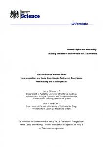
The HILDA Survey data shows that in 2006 just over 60% of Australians aged 15 and over were legally or de facto married, around a quarter had never been married and were not living with a partner, 7% were separated or divorced and had not re-partnered and the remaining 6% were widows or widowers. Figure 2.1 shows that there has been very little change in these proportions over the six years from 2001 to 2006. In 2006, there were 114,222 registered marriages— the highest number of marriages since 1999 and an increase of 4.5% from 2005 (Australian Bureau of Statistics (ABS), 2007a). The number of divorces in 2006 in Australia was 51,375—a decrease of 2% from 2005, and the fifth annual decrease since a high of 55,330 divorces in 2001 (ABS, 2007b). Table 2.1 summarises the changes in marital status among HILDA Survey respondents who were interviewed in both 2005 and 2006. Most people (98%) who were married in 2005 were still married in 2006. Of those who were in a de facto relationship in 2005, 10% had married and 11% were no longer living with a partner by 2006. A small proportion, 5%, of people who were divorced in 2005 were now in a de facto relationship, as were 7% of those who had never married

and were not in a de facto relationship in 2005.1 While things remained relatively stable during this 12 month period, a lot more happened over the five years from 2001 to 2006, as shown in Table 2.2. In the six years from 2001 to 2006, the most stable group was the widowed, with 98% retaining that status in 2006. Of those who were married in 2001, 92% were married in 2006—to the same person in 99% of cases. Of those whose marital status in 2001 was divorced, 9% had re-married by 2006 and a further 8% were cohabiting with a partner. Just over one-quarter of people who were never married and not living with a partner in 2001 had a partner by 2006, 15% had moved into a de facto relationship and 12% were married. The most volatile groups seem to be separated people and those in de facto relationships. However, most of the separated people who had changed marital status after 2001 had proceeded with a divorce; 32% of de factos who changed status after 2001 got married; 97% of them marrying the person they were living with in 2001. Furthermore, among those who were in de facto relationships in both 2001 and 2006, 85% were still living with the same partner.

Figure 2.1: Marital status at time of interview 60

50 Legally married Never married and not currently de facto married

40

De facto married % 30

Divorced Widowed

20

Separated

10

0 2001

2002

2003

2004

2005

2006

Note: Population weighted results.


5

Households and Family Life Relationship satisfaction Each year, individuals living with a spouse or partner at the time of their interview are asked to rate their satisfaction with their relationship with their partner, on a scale of 0 (completely dissatisfied) to 10 (completely satisfied). Average levels of relationship satisfaction by sex and marital status are shown in Figure 2.2. Compared to people in de facto relationships, relationship satisfaction was higher, on average, among married persons. In 2006, the average level of relationship satisfaction for married males was 8.6 out of 10, compared to 8.4 out of 10 for males in de facto relationships. For females, the average level of relationship satisfaction was only slightly higher for those married—8.3 out of 10 compared to 8.2 out of 10 for females in a de facto relationship. Using the 2005 HILDA Survey data, Headey and Warren (2008) found that, on average, individuals married for less than two years report the highest levels of relationship satisfaction; for males, average relationship satisfaction dropped to 8.5 out of 10 after two years of marriage and for females, average relationship satisfaction also dropped to 8.5 out of 10 for those who had been married for between two and five years, and down to 8.1 out of 10 for females who had been married for five

years or longer. The question remains, however, how much does relationship satisfaction change in a year? Table 2.3 compares relationship satisfaction in 2005 and 2006 for individuals who were married or in a de facto relationship in 2005. Most married people—90% in the case of men and 89% in the case of women—who reported high levels of relationship satisfaction in 2005, also reported high levels of satisfaction in 2006. Of those married persons who reported medium levels of relationship satisfaction—4 to 7 out of 10— 40% of males and 38% of females reported high levels of satisfaction with their relationship in 2006. For a substantial proportion of married people, it seems that low levels of relationship satisfaction were temporary, with 69% of married men and 57% of married women who reported low levels of relationship satisfaction in 2005— 3 out of 10 or lower—reporting an improvement in relationship satisfaction by 2006. For some this may have only been a slight improvement, but for almost 40% of married men who reported low levels of relationship satisfaction in 2005, it was an improvement to 8 or higher out of 10 by 2006. Compared to married couples, de facto relationships were much less stable, with 58% of men and 48% of women who reported relationship satisfaction of 7

Table 2.1: Changes in marital status, 2005–2006 (%)

Marital status in 2006

Marital status in 2005 Legally married De facto Separated Divorced Widowed Never married and not de facto Total

Legally married 98.3 9.5 *4.8 *1.2 *0.3 1.8 55.5

De facto *0.1 80.0 6.5 5.2 *0.3 7.3 9.4

Separated 1.0 0.6 71.7 2.2 0.6 *0.2 2.9

Divorced *0.0 1.7 17.0 89.1 2.1 *0.0 6.5

Widowed 0.5 *0.1 *0.0 2.3 96.7 *0.0 6.3

Never married and not de facto – 8.1 – – – 90.6 19.4

Total 100.0 100.0 100.0 100.0 100.0 100.0 100.0

Never married and not de facto – 10.8 – – – 72.5 19.1

Total 100.0 100.0 100.0 100.0 100.0 100.0 100.0


Table 2.2: Changes in marital status, 2001–2006 (%)

Marital status in 2006

Marital status in 2001 Legally married De facto Separated Divorced Widowed Never married and not de facto Total

Legally married 92.0 32.4 9.7 8.6 *0.5 11.9 55.4

De facto 0.9 49.5 11.6 8.0 *0.1 14.5 9.2

Separated 2.3 2.3 43.8 *0.8 *0.0 *0.7 2.9

Divorced 1.5 4.4 30.0 76.8 *1.7 *0.3 6.2

Widowed 3.2 *0.6 4.9 5.8 97.6 *0.1 7.2


6


Households and Family Life or lower in 2005 no longer living with their partner in 2006. Still, 40% of males and 22% of females who reported medium levels of relationship satisfaction in 2005 rated their satisfaction with their relationship as 8 or higher out of 10 in 2006. 76% of males and 78% of females who had high levels of relationship

satisfaction in 2005—8 or higher out of 10—also reported high levels of satisfaction in 2006. Table 2.3 suggests that people make more effort to save a marriage than to stay in a de facto relationship, with less than 2% of marriages ending compared to more than 10% of de facto relationships.

Figure 2.2: Mean satisfaction with partner (0–10 scale) Men

9

Women

9

8.8

8.8

Married De facto 8.6

8.6

8.4

8.4

8.2

8.2

8

8

7.8

7.8 2001

2002

2003

2004

2005

2006

2001

2002

2003

2004

2005

2006


Table 2.3: Changes in relationship satisfaction of married persons, 2005–2006 (%)

Relationship satisfaction in 2005 Males—married Low (0–3) Medium (4–7) High (8–10) Total Females—married Low (0–3) Medium (4–7) High (8–10) Total Males—de facto Low (0–3) Medium (4–7) High (8–10) Total Females—de facto Low (0–3) Medium (4–7) High (8–10) Total

Low (0–3)

Relationship satisfaction in 2006 Medium High No longer in (4–7) (8–10) relationshipa

Total

*27.7 5.8 *1.0 2.6

31.0 51.6 7.6 15.5

38.3 40.2 90.4 80.6

*3.0 *2.3 1.0 1.3

100.0 100.0 100.0 100.0

37.2 4.7 *0.7 2.9

38.7 54.9 9.3 20.3

*18.0 38.4 88.6 75.0

*6.1 2.0 1.4 1.7

100.0 100.0 100.0 100.0

*6.6 *3.4 *1.6 *2.2

*19.5 40.5 12.0 18.6

*20.3 39.5 76.1 65.8

*53.6 *16.6 10.4 13.4

100.0 100.0 100.0 100.0

*22.2 *10.1 *3.3 5.7

*35.0 51.9 10.9 22.8

*11.4 21.7 78.1 60.6

*31.4 16.3 7.7 10.8

100.0 100.0 100.0 100.0

Notes: Population weighted results. * Estimate not reliable. a Includes all individuals who were not living with the same spouse or partner from the previous year. For most (85.8%) this was because the relationship had broken up. Percentages may not add up to 100 due to rounding.


7


Table 2.4: Changes in relationship satisfaction of married persons, 2001–2006 (%)

Relationship satisfaction in 2001 Males—married Low (0–3) Medium (4–7) High (8–10) Total Females—married Low (0–3) Medium (4–7) High (8–10) Total Males—de facto Low (0–3) Medium (4–7) High (8–10) Total Females—de facto Low (0–3) Medium (4–7) High (8–10) Total

Low (0–3)

Relationship satisfaction in 2006 Medium High No longer in (4–7) (8–10) relationshipa

Total

*14.6 *6.4 1.4 2.3

*37.4 37.8 11.4 15.0

*21.5 44.1 81.6 76.0

*26.5 11.7 5.6 6.7

100.0 100.0 100.0 100.0

28.4 8.4 1.1 3.0

*21.6 41.1 14.1 18.6

*16.9 36.1 77.1 68.9

33.0 14.3 7.7 9.5

100.0 100.0 100.0 100.0

*10.5 *1.3 *1.2 *1.4

*0.0 35.5 12.3 16.2

*0.0 33.9 69.0 61.4

*89.5 29.3 17.6 21.1

100.0 100.0 100.0 100.0

*15.4 *8.6 *2.7 *4.3

*0.0 34.5 17.4 20.1

*16.0 26.2 59.6 51.2

*68.6 30.7 20.3 24.3

100.0 100.0 100.0 100.0

Notes: Population weighted results. * Estimate not reliable. a Includes all individuals who were not living with the same spouse or partner from 2001. For most (79.6%) this was because the relationship had broken up. Percentages may not add up to 100 due to rounding.

Table 2.4 compares levels of relationship satisfaction for married persons and those in de facto relationships between 2001 and 2006 and leads to the expected conclusion that happy relationships continue and unhappy ones usually do not. While 82% of married men and 77% married of women who had reported high levels of relationship satisfaction in 2001 were still very happy with their relationship in 2006, 6% of men and 8% of women were no longer married. The proportion of people who were no longer living with their spouse or partner from 2001 was much higher for those who were less satisfied with their relationship in 2001; 12% of men and 14% of women who were married in 2001 and reported medium levels of relationship satisfaction were no longer married, and one-third of women and around one-quarter of men who reported levels of relationship satisfaction of 3 out of 10 or less were no longer married. Only 69% of men and 60% of women who reported high levels of satisfaction with their de facto relationship were still highly satisfied with their relationship in 2006. The majority of the individuals who reported low levels of satisfaction

8


with their de facto relationship in 2001 were no longer living with that partner in 2006. Overall, around 30% of people who reported medium levels of satisfaction and 20% of people who reported high levels of satisfaction with their relationship with their de facto relationship in 2001 were no longer living with their partner by 2006. Endnote 1

This refers to all those whose marital status in 2005 was divorced, not people whose divorce was finalised in 2005.

References Australian Bureau of Statistics (2007a) Marriages, Australia, 2006, ABS Catalogue No. 3306.0.55.001, Canberra. Australian Bureau of Statistics (2007b) Divorces, Australia, 2006, ABS Catalogue No. 3307.0.55.001, Canberra. Headey, B.W. and Warren, D. (2008) Families, Incomes and Jobs, Volume 3: A Statistical Report on Waves 1 to 5 of the HILDA Survey, Melbourne Institute of Applied Economic and Social Research, Melbourne.


3.

Parenting stress and work–family stress

Most parents feel stressed from time to time. This stress may be a result of juggling work and family arrangements, finding adequate child care, taking care of ill or disabled children, parenting adolescents or teenagers, troubles getting along with stepchildren, or just the general daily stresses associated with being a parent. In each year of the HILDA Survey, individuals with parenting responsibilities for children aged 17 or younger are asked how strongly they agree or disagree with statements related to parenting stress like, ‘I feel trapped by my responsibilities as a parent’ and ‘I find that taking care of my child is much more work than pleasure’. The response scale runs from 1 (strongly disagree) to 7 (strongly agree). Table 3.1 compares the distribution of responses to the questions about parenting stress in 2006 for lone parents and parents who have a spouse or partner. It is much more common for women than men to agree with the statements ‘Being a parent is harder than I thought it would be’ and ‘I often feel tired, worn out or exhausted from meeting the needs of my children’, and compared to mothers

who had a spouse or partner, it is more common for lone mothers to agree with these statements. Although the proportion of parents who reported strong agreement with the statements ‘I feel trapped by my responsibilities as a parent’ and ‘I find that taking care of my children is much more work than pleasure’, is relatively small, a higher proportion of lone parents agreed with the statements. In previous HILDA Statistical Reports, it was found that, based on a measure of parenting stress calculated by taking the average of the responses to the four statements in Table 3.1, the majority of parents fall into the category of ‘medium’ parenting stress—3 to 5 out of 7. Sole parents reported higher levels of parenting stress than parents who were married or in a de facto relationship. Table 3.2 shows the proportion of parents who reported high levels of parenting stress—6 or 7 out of 7— in the six years from 2001 to 2006. The proportion of parents who reported high levels of parenting stress dropped by just over 4% since 2001, from 12% in 2001 to 7% in 2006. In 2006, 13% of lone mothers reported high levels of parenting stress, compared to 9% of partnered

Table 3.1: Parenting stress, 2006 (%)

Stress level Strongly disagree 1 2 3 4 5 Being a parent is harder than I thought it would be Lone mothers 7.0 8.7 12.5 12.3 23.4 Partnered mothers 7.0 13.8 10.7 14.4 22.1 Lone fathers *9.9 8.6 15.3 25.3 20.3 Partnered fathers 8.5 15.6 16.3 22.1 19.8 Total 7.7 13.8 13.4 17.8 21.2 I often feel tired, worn out or exhausted from meeting the needs of my children Lone mothers 5.7 11.9 11.6 21.1 19.1 Partnered mothers 4.9 14.1 11.8 17.0 21.3 Lone fathers *7.1 17.5 15.6 21.4 20.9 Partnered fathers 7.6 20.6 17.4 22.4 18.1 Total 6.2 16.7 14.3 19.9 19.7 I feel trapped by my responsibilities as a parent Lone mothers 26.8 23.8 12.4 16.1 9.8 Partnered mothers 29.1 27.5 15.1 12.9 7.3 Lone fathers 18.5 32.7 16.2 *7.2 *11.9 Partnered fathers 26.9 32.3 15.0 12.7 7.5 Total 27.4 29.3 14.8 12.9 7.9 I find that taking care of my children is much more work than pleasure Lone mothers 24.8 19.4 14.2 19.4 12.6 Partnered mothers 26.7 27.8 15.2 13.4 8.9 Lone fathers 18.8 36.2 19.4 9.7 *7.3 Partnered fathers 21.4 31.9 19.1 14.6 6.7 Total 23.9 28.9 16.9 14.4 8.3

6

Strongly agree 7

Total

Mean stress level

16.5 19.4 12.3 12.5 15.9

19.6 12.5 *8.3 5.3 10.1

100.0 100.0 100.0 100.0 100.0

4.6 4.4 4.1 3.9 4.2

16.1 20.1 13.6 10.3 15.3

14.6 10.8 *3.9 3.6 7.9

100.0 100.0 100.0 100.0 100.0

4.4 4.4 3.9 3.7 4.1

7.0 5.1 *9.8 4.0 5.1

4.1 2.9 *3.7 1.6 2.6

100.0 100.0 100.0 100.0 100.0

3.0 2.7 3.1 2.6 2.7

2.7 5.3 *3.5 4.2 4.5

6.8 2.7 *5.0 2.1 3.0

100.0 100.0 100.0 100.0 100.0

3.1 2.8 2.8 2.7 2.8



9

Households and Family Life mothers and only 4% of partnered fathers who were living with a spouse or partner. In all six years, women reported substantially higher levels of parenting stress than men, lone mothers had higher stress levels than partnered mothers and, in all but one year, lone fathers reported higher levels of stress than partnered fathers. Is parenting stress higher for parents with young children? How does the age of the children in the household affect parenting stress? Is parenting stress higher for people with young children, or are teenagers the most troublesome? Table 3.3 shows the proportion of parents with high levels of parenting stress (6 or 7 out of 7) in 2006, by the sex and marital status of the parent and the age of the youngest child in the household. In general, parents whose youngest child was under the age of 13 had slightly higher levels of parenting stress, with just over 7% reporting stress levels of 6 or higher out of 7, compared to 6% of parents whose youngest child was aged between 13 and 17.1 However, partnered fathers seemed to escape this stress, with only 4% reporting high levels of parenting stress, compared to 9% of part-

nered mothers, 11% of lone fathers and 13% of lone mothers. Compared to partnered mothers whose youngest child was not yet a teenager, partnered mothers whose youngest child was aged between 13 and 17 were less stressed, with 7% reporting high levels of parenting stress, compared to over 9% of partnered mothers whose youngest child was under the age of 13. One would also expect that the level of stress that parents feel would be higher if they have more than one child. In 2006, the proportion of parents with high levels of parenting stress ranged from 7% for parents whose children were all aged six or older, to 10% for parents with three or more children all under the age of six. Only 5% of parents with one child under the age of 19 reported high levels of parenting stress, compared to 6% of parents with two children under the age of 18 and 11% of parents with three or more children under 18.2 Table 3.4 shows the correlation between parenting stress and the age of the youngest child, as well as the correlations between parenting stress and the number of children aged five and under, and the number of children under 18. A weak negative correlation between parenting stress and the age of the youngest child is evident

Table 3.2: Proportion of parents with high levels of parenting stress by sex and marital status (%) Lone mothers Partnered mothers Lone fathers Partnered fathers Total

2001 16.9 13.7 11.8 7.6 11.5

2002 17.0 11.6 *5.1 5.5 9.4

2003 15.7 9.6 *6.9 4.8 8.2

2004 14.1 9.0 *8.2 4.3 7.7

2005 16.9 9.0 9.9 4.1 8.0

2006 12.9 9.1 *11.4 3.7 7.4

Notes: Population weighted results. * Estimate not reliable.

Table 3.3: Proportion of parents with high levels of parenting stress by sex, marital status and age of youngest child, 2006 (%)

Age of youngest child 3–5 6–12 *15.4 *10.6 9.9 9.4 *2.6 *8.1 *2.8 3.8 7.2 7.2

0–2 *13.8 9.0 *16.5 3.8 7.1

Lone mothers Partnered mothers Lone fathers Partnered fathers Total

13–17 *9.8 6.9 *15.0 *2.2 6.4

Total 12.9 9.1 11.4 3.7 7.4


Table 3.4: Parenting stress by age of youngest child and number of children—Correlations by sex and marital status, 2006 Lone mothers Partnered mothers Lone fathers Partnered fathers Total Note:

10

#

Age of youngest child –0.086^ –0.074 –0.130# –0.072# –0.061#

Number of children under 6 0.088^ 0.065# –0.053 0.065# 0.056#

and ^ indicate correlation is significant at the 5% level and 10% level respectively.


Number of children under 18 0.189# 0.106# 0.102 0.117# 0.113#

Households and Family Life in Table 3.4. In other words, as the age of the youngest child increases, parenting stress decreases slightly, particularly for lone fathers. On the other hand, there is a strong positive correlation between levels of parenting stress and the number of children under the age of 18, especially for lone mothers. Parenting stress also increases slightly with the number of children aged five or younger. Work–family stress Parents in paid work are also asked how strongly they agree or disagree with statements relating to work–family stress. Table 3.5 compares the average responses to the questions about work–family stress in 2006 for lone parents and parents who

have a spouse or partner, according to whether they work full-time or part-time. Apart from the small group of lone fathers who work full-time, lone mothers who are working either full-time or part-time have the highest levels of work–family stress. Partnered fathers on the other hand, have the lowest average work–family stress levels.3 It is slightly more common for lone mothers, working either full-time or part-time, to say that they have turned down work opportunities because of family responsibilities. Compared to parents who work part-time, it is more common for parents who are in full-time work to say that the time they spend at work is less enjoyable and more pressured because of family responsibilities, that they miss out

Table 3.5: Work–family stress, 2006 (means)

Because of my family Because of Because of the responsibilities, I my family requirements of Because of the have to turn down responsibilities, my job, I miss requirement of work activities the time I spend out on home or my job, my or opportunities working is less family activities family time is less that I would prefer enjoyable and that I would prefer enjoyable and to take on more pressured to participate in more pressured Employed full-time Lone mothers Partnered mothers Lone fathers Partnered fathers Employed part-time Lone mothers Partnered mothers Lone fathers Partnered fathers Total

Overall work–family stress

3.6 3.3 3.3 3.2

3.4 3.3 3.5 3.2

4.3 4.3 4.2 4.4

3.7 3.7 3.6 3.5

3.8 3.6 3.5 3.4

3.8 3.3 *3.6 3.4 3.3

3.4 3.0 *3.0 2.9 3.2

3.6 3.2 *2.9 3.7 4.1

3.1 2.8 *2.2 2.6 3.3

3.8 3.7 *4.2 3.4 3.5


Table 3.6: Proportion of parents with high levels of work–family stress by sex, marital status and working hours (%)

Employed full-time Lone mothers Partnered mothers Lone fathers Partnered fathers Employed part-time Lone mothers Partnered mothers Lone fathers Partnered fathers All employed Lone mothers Partnered mothers Lone fathers Partnered fathers Total

2001

2002

2003

2004

2005

2006

*10.5 9.5 *7.9 6.6

*13.1 11.1 *4.9 6.8

*13.8 9.9 *8.2 5.4

*10.4 7.1 *4.7 4.9

*15.5 8.5 *15.1 6.4

*10.6 10.2 *6.3 6.3

*7.3 4.9 *10.8 *10.2

*9.6 5.8 *0.0 *3.6

*7.1 4.8 *0.0 *5.6

*5.9 5.2 *9.8 *3.7

*7.5 3.2 *10.0 *7.2

*8.2 4.8 *0.0 *1.0

9.2 7.0 *8.6 7.2 7.4

11.3 7.8 *4.5 6.6 7.3

10.3 6.8 *6.3 5.4 6.4

8.2 5.9 *5.2 4.9 5.6

11.0 5.3 *13.8 6.4 6.8

9.7 7.0 *5.3 6.1 6.7



11

Households and Family Life on family activities because of the requirements of their job, and that family time is less enjoyable and more pressured because of their work requirements.

or part-time) reported high levels of work–family stress, compared to 7% of partnered mothers. Persistence of family-related stress, 2001 to 2006

Looking at average levels of work–family stress does not reveal much variation between the stress levels of parents who work full-time or part-time, or differences between men and women. Table 3.6 shows the proportion of parents who reported high levels of work–family stress (6 or 7 out of 7) in the six years from 2001 to 2006.

In previous HILDA Statistical Reports, it was found that while some parents manage to reduce their parenting stress, for others the problem persists for a fairly long time. For example, 25% of men and 32% of women who had high parenting stress in 2001 still had high levels in 2004, and only 15% of men and 3% of women had managed to reduce high levels of stress to low. Tables 3.7 and 3.8 compare the levels of parenting stress and work– family stress in 2005 and 2006 for persons who had parenting responsibilities in both years.

Overall, levels of work–family stress have dropped slightly since 2001. The proportion of parents who were employed full-time and reported high levels of work–family stress dropped from 7% in 2001 to 6% in 2004 and then increased to 7% in 2006. In all six years, it was more common for parents who work full-time to report higher levels of stress than parents who work part-time. This is particularly the case for partnered mothers. In 2006, 10% of partnered mothers who worked full-time reported high levels of work–family stress, compared to 5% of partnered mothers who were working part-time. Compared to mothers with partners, it is more common for lone mothers to report high levels of work–family stress. In 2006, 10% of lone mothers (who were working either full-time

Of those parents who reported high levels of parenting stress in 2005, 29% of fathers and 53% of mothers also reported high parenting stress levels in 2006. This suggests that for mothers, parenting stress does persist for some time. Over 80% of parents who reported medium levels of parenting stress in 2005—3 to 5 out of 7—also reported medium levels in 2006, while over 40% of people who reported low levels of parenting stress in 2005 had medium levels of stress by 2006. Of

Table 3.7: Persistence of parenting stress, 2005–2006 (%)

Parenting stress in 2005 Males Low (1–2) Medium (3–5) High (6–7) Total Females Low (1–2) Medium (3–5) High (6–7) Total

Low (1–2)

Parenting stress in 2006 Medium (3–5)

High (6–7)

Total

58.6 16.1 *4.7 24.6

40.8 80.2 66.2 71.3

*0.5 3.7 29.0 4.1

100.0 100.0 100.0 100.0

56.8 11.3 *2.0 17.2

43.2 82.9 44.6 72.2

*0.0 5.9 53.4 10.5

100.0 100.0 100.0 100.0


Table 3.8: Persistence of work–family stress, 2005–2006 (%)

Work–family stress in 2005 Males Low (1–2) Medium (3–5) High (6–7) Total Females Low (1–2) Medium (3–5) High (6–7) Total

Low (1–2)

Work–family stress in 2006 Medium (3–5) High (6–7)

52.0 10.8 *0.0 18.1

47.4 84.4 80.6 76.8

*0.6 4.9 19.4 5.1

100.0 100.0 100.0 100.0

53.2 14.5 *0.0 22.9

45.7 78.8 51.7 69.1

*1.0 6.7 48.3 8.0

100.0 100.0 100.0 100.0


12

Total


Households and Family Life course, the household situation may have changed during this time. For example, parents may have separated or had a new baby, causing higher levels of stress for one or both parents. On the other hand, the stress may have eased for parents whose children are now school age and more able to look after themselves. Parents’ working hours may also have changed—increased work hours of either parent may increase levels of work–family stress, while reducing work hours may have the opposite effect. In terms of work–family stress, almost half the mothers who reported high levels of work–family stress in 2005 also had high levels of stress in 2006. However, of the fathers who reported high levels of work–family stress in 2005, only 19% were still highly stressed in 2006. Just under 80% of mothers and 84% of fathers who reported medium levels of work–family stress in 2005 still had medium levels of stress in 2006, while more than 45% of mother and fathers whose work–family stress was low in 2005 had medium levels of stress in 2006. Tables 3.7 and 3.8 show that it is much more common for women than men to experience high levels of parenting stress and work–family stress that continues for at least one year, but Tables 3.9

and 3.10, which compare the levels of parenting stress and work–family stress in 2001 and 2006 for individuals with parenting responsibilities in both 2001 and 2006, show that most parents are able to reduce their stress in the longer-term. While very few parents who reported high levels of parenting stress in 2001 had reduced their stress levels to low by 2006, 72% of men and 66% of women who reported high levels of parenting stress in 2001 had medium levels of parenting stress in 2006. Just over three-quarters of parents who said their parenting stress was medium in 2001 reported medium levels in 2006, while 20% of men and 17% of women had gone from having medium levels of parenting stress in 2001 to low levels in 2006. Around half the parents who reported low levels of parenting stress in 2001 reported medium levels of parenting stress in 2006, but very few had gone from low levels of parenting stress in 2001 to high parenting stress in 2006. Similar to the pattern evident for parenting stress, Table 3.10 shows that, of those who reported high levels of work–family stress in 2001, few had been able to reduce their stress to low: 83% of men and 65% of women had lowered their level of work–family stress to medium, leaving 15% of

Table 3.9: Persistence of parenting stress, 2001–2006 (%)

Parenting stress in 2001 Males Low (1–2) Medium (3–5) High (6–7) Total Females Low (1–2) Medium (3–5) High (6–7) Total

Low (1–2)

Parenting stress in 2006 Medium (3–5)

High (6–7)

Total

50.3 20.3 *2.9 25.5

49.0 76.8 72.2 70.7

*0.7 2.9 24.9 3.8

100.0 100.0 100.0 100.0

46.5 16.5 *4.5 18.7

52.6 76.7 65.5 71.8

*1.0 6.8 30.0 9.5

100.0 100.0 100.0 100.0


Table 3.10: Persistence of work–family stress, 2001–2006 (%)

Work–family stress in 2001 Males Low (1–2) Medium (3–5) High (6–7) Total Females Low (1–2) Medium (3–5) High (6–7) Total

Low (1–2)

Work–family stress in 2006 Medium (3–5) High (6–7)

Total

37.6 13.6 *2.8 17.7

58.8 82.0 82.7 77.2

*3.6 4.4 14.5 5.0

100.0 100.0 100.0 100.0

45.0 13.2 *3.9 20.8

52.8 78.4 65.2 70.4

*2.3 8.3 31.0 8.8

100.0 100.0 100.0 100.0



13

Households and Family Life men and 31% of women who reported high levels of work–family stress in both 2001 and 2006. As with parenting stress, well over 50% of people with low levels of stress in 2001 reported medium levels of work–family stress in 2006, and approximately 80% of parents who reported medium levels of work–family stress in 2001 also reported medium stress levels in 2006. These results suggest that while many are able to reduce their levels of parenting stress and work– family stress to some extent, ‘medium’ levels of stress seem to persist for several years, and high levels of parenting stress and work–family stress are more persistent for mothers than for fathers.

4.

Endnotes 1

It should be noted that we are not implying that stress is related only to the age of the youngest child. There could be a combination of factors causing the stress, for example, a parent of a 5 year old and a teenage child may be stressed because of the older child.

2

There are too few cases to break down these figures by sex and marital status, therefore correlations are shown.

3

There is no significant correlation between age of youngest child and work–family stress observed for men or women. There is only a slight positive correlation (0.063) between work–family stress and the number of children under 18 for coupled men, while all other groups have no significant correlation.

Child care: Issues and persistence of problems

Issues related to child care have become more important over the last two decades. Changes in female employment patterns and changes in family structures—for example, a growing number of lone parent families—have created a growing need for child care that is both accessible and affordable. According to the Australian Institute of Health and Welfare (2005), 61,000 Australian children were prevented from attending child care in 2003 because of a lack of child care places; a further 30,000 children were not in child care because the cost was too high; and 22,000 could not access a place because there were none in the area. Table 4.1 shows the proportion of households with children under 15, as well as the proportion of households who had used or had considered using child care in the 12 months prior to their interview for the five years from 2002 to 2006.1 Work-related child care is more common than non-work-related child care; in 2006, 45% of households with children under 15 using workrelated child care, and 23% using child care while the parents are doing non-work-related activities. In all five years, approximately 28% of households had at least one child aged 14 or younger living in the household. In those households with children

aged 14 or less, approximately half had either used or considered using child care. The proportion of households with children aged 14 or younger who used some type of child care while the parents were at work increased from 40% of households in 2002 to 45% in 2006, while the proportion of households with children under the age of 15 who used child care while the parents were not at work declined slightly—from 26% of households in 2002 to 23% of households in 2006. Child care in 2006 In previous HILDA Statistical Reports, it was found that the use of child care is most common in households with children aged between two and five years. Figure 4.1 shows the proportion of households with children aged 14 or younger who used child care in 2006, broken down by the age of the children in the household. In 2006, use of work-related and non-work-related child care was most common in households with at least one child between the ages of two and five. While more than half of the parents in households where at least one child was under 10 years of age had used or considered using some form of child care, only 43% of households with children aged between 10 and 12 and 31% of households with

Table 4.1: Child care use (%) Proportion of households with children aged 14 or less Of those with children aged 14 or less… Proportion who used or considered using child care in the past 12 months Proportion who used work-related child care in the past 12 months Proportion who used non-work-related child care in the past 12 months

2002

2003

2004

2005

2006

28.6

28.5

28.3

28.0

27.6

49.5

49.6

49.0

49.2

51.1

40.3

40.8

42.2

41.3

44.8

26.3

26.4

26.5

24.3

23.2


14



Figure 4.1: Child care use, by age of children, 2006 70

60

50

40 % 30

20

10

0

0 in 2002 (%) Mean Median Assets Value of own home 70.6 79,180 80,124 82.9 33,299 15,249 Superannuation 18.0 145,194 –3,541 Value of other property 41.2 13,122 –1,573 Equity investments 15.1 –126,183 –22,485 Value of own business Other assets 99.7 7,933 730 Debts Home debt 40.5 –3,674 –12,075 8.6 –45,542 –58,634 Other property debt 33.8 205 –562 Credit card debt 43.9 –4,109 –4,112 Other personal debt Business debt 6.5 –85,832 –28,106

10th percentile

90th percentile

–93,170 –57,889 0 –16,863 –3,727 –68,257

306,521 136,003 280,000 20,634 8,758 75,715

–67,268 0 –1,907 –16,863 0

160,062 0 3,595 20,000 0

10th percentile

90th percentile

–166,959 –79,820 –361,340 –76,691 –674,536 –68,257

276,397 158,452 550,308 82,546 387,577 75,715

–146,150 –297,920 –5,621 –36,938 –292,299

157,639 125,464 6,814 26,019 37,752

Notes: Population weighted results. All monetary values expressed at September quarter 2006 prices.


99

Household Wealth Endnotes 1

The questions on wealth in the wave 6 survey were very similar to the wealth questions in the wave 2 survey, ensuring a high degree of comparability of wealth measures across the two waves. There are two minor differences in the questions. First, in 2006, separate information for each of six ‘other personal debt’ components was obtained, whereas in 2002 only the total of these components was obtained. Second, in 2006 the value of unpaid household bills was obtained separately.

2

In part, the difference reflects the fact that wealth is not adjusted for household size (equivalised) as is done for income.

3

Note that the Gini coefficient excludes persons with negative net worth, which may explain the fact that the Gini coefficient did not decline as did the percentile ratios.

4

The growth in millionaires would be even greater if wealth in 2002 had not been scaled up to September 2006 prices.

5

In part, the apparent weakness of the association between income and wealth at low levels of income can be attributed to given dollar-value changes in wealth at low wealth levels representing bigger proportionate changes than they do at high wealth levels. The apparent ordering of wealth inequality by income level may also be at least partially an artefact of given dollar values translating to smaller percentage changes at higher wealth levels.

Reference Australian Bureau of Statistics (2009) House Price Indexes: Eight Capital Cities, ABS Catalogue No. 6416.0, Canberra.

22. Experiences of people with the smallest and largest increases in wealth between 2002 and 2006 What happened to the people with the largest increases in wealth, and to the people whose wealth increased the least—or indeed fell? Are there systematic differences in experiences and outcomes of those with the biggest gains and those with the smallest gains? Or do differences in wealth accumulation simply reflect differences in characteristics, preferences (e.g. propensity to save) and various random factors (such as luck in winning a lottery)? We can use the information collected by the HILDA Survey in all of the years between 2002 and 2006 to describe the characteristics and experiences of people with the smallest wealth gains, and people with the largest wealth gains, in order to shed light on these questions. We define the ‘smallest gains’ and ‘largest gains’ groups as follows. The median of each decile of the 2002 net worth distribution is identified, and then each individual’s change in household wealth is expressed as a proportion of the median of the decile of the 2002 distribution to which the individual belonged. This produces a measure of each individual’s proportionate change in net worth that reduces the occurrence of extreme values caused by very low initial wealth. For example, any change in net worth is of infinite magnitude in percentage terms if an individual has zero initial net worth. Note also that expressing changes simply in terms of ‘dollar changes’ is not a desirable alternative to a ‘proportionate change’ measure, because it will over-represent the wealthy in both the smallest-increase and biggestincrease groups, since they tend to have the largest dollar changes in wealth, in both upward and downward directions.

100


Given the above measure of wealth change, we then assign each individual to a quintile of the distribution of changes. Those allocated to the bottom quintile—the 20% of the population with the lowest percentage increases in net worth— constitute the ‘lowest-increase’ group. Those allocated to the top quintile—the 20% of the population with the largest percentage increases in net worth—constitute the ‘biggest-increase’ group. For all of the analysis, we exclude persons under 25 years of age in 2002. The primary motivation is that many children will move out of the parental home between 2002 and 2006 and are then likely to dominate the low-growth group because of the precipitous decline in household (but not personal) wealth that accompanies the move. Such sources of wealth changes are of little interest from a research or policy perspective.1 Our analysis is therefore of individuals who, in 2002, were ‘Smallest wealth-gain’ and ‘largest wealth-gain’ groups For the purposes of identifying the two ‘wealth-gain’ groups, an individual’s ‘wealth-gain’ is defined to be the change in household net worth of that individual between 2002 and 2006 relative to the median (midpoint) of the 2002 wealth decile to which the individual belonged. Individuals are then sorted by wealthgain from lowest to highest, with the bottom 20% comprising the ‘smallest wealth-gain’ group (some or all of whom may have experienced declines in wealth) and the top 20% of people comprising the ‘largest wealth-gain’ group.

Household Wealth

Table 22.1: Wealth of those with the least growth in wealth and those with the greatest growth in wealth Median wealth in 2002 ($) Median wealth in 2006 ($) Median growth in wealth (%)

Least growth in wealth 406,127 186,000 –52.2

Greatest growth in wealth 76,470 372,500 325.5

All persons 316,613 427,891 35.2

Note: Population weighted results. Population is persons over 25 years of age in 2002.

over the age of 25 years, which is in any case the age at which the issue of wealth accumulation takes on significance. Furthermore, it is when individuals are over 25 years of age that their experiences and outcomes are likely to be relevant to wealth accumulation. Table 22.1 provides details on the wealth levels and growth of the two groups. Median wealth in 2002 was $406,127 for the low-growth group and $76,470 for the high-growth group. Thus, the lowgrowth group tends to be those who initially held considerable wealth, and the high-growth group tends to be those with relatively little to begin with. The median proportionate growth was –52.2% for the low-growth group and 325.5% for the high-growth group.

Characteristics of the wealth-gain ‘winners’ and ‘losers’ Table 22.2 compares demographic characteristics of individuals with the lowest growth in wealth and individuals with the greatest growth in wealth. The distribution of these individuals across the basic four household types is not greatly different. Those in the low-growth group are less likely to be in couple households with or without children than those in the high-growth group, and somewhat more likely to be in single-person households. Both groups are less likely to be in couple households without children in 2002 than the general population, and both are more likely to be in lone parent households in 2002. The two groups do, however, have differences in the number of

Table 22.2: Demographic characteristics in wave 2 of those with the least growth in wealth and those with the greatest growth in wealth

Least growth in wealth Type of household (%) Couple, no children Couple with children Lone parent Other Total Mean number of children aged under 15 years Age group (%) 25–34 years 35–44 years 45–54 years 55–64 years Over 65 years Total Educational attainment (%) Degree or higher Diploma or Certificate III/IV High school Certificate I/II Year 10/11 Less than Year 10 Total Full-time student (%) Mean general health (SF–36) Disabled (%) Disability in household (%) Home owner (%)

Greatest growth in wealth

All persons

24.3 39.8 11.6 24.2 100.0 0.6

26.5 43.4 11.0 19.1 100.0 0.8

29.9 42.8 8.7 18.6 100.0 0.6

24.7 21.6 20.6 15.8 17.2 100.0

38.3 29.7 16.2 9.8 6.0 100.0

22.3 24.5 22.0 15.3 15.9 100.0

15.7 30.1 13.3 1.6 22.0 17.3 100.0 17.2 66.6 28.9 43.5 67.3

20.8 27.1 13.1 2.6 23.3 13.2 100.0 10.3 70.0 20.0 31.2 52.6

18.9 29.0 12.2 2.0 23.3 14.5 100.0 9.5 68.5 23.7 36.7 75.3

Notes: Population weighted results. Population is persons over 25 years of age in 2002. Percentages may not add up to 100 due to rounding.


101

Household Wealth dependent children, people in the low-growth group averaging 0.6 children per household and people in the high-growth group averaging 0.8 children per household. The age profiles of the low- and high-growth groups differ considerably. Consistent with the prime-age years being the main wealth accumulation years, the high-growth group is predominately between 25 and 45 years of age. The low-growth group, by contrast has relatively high proportions in the young and older age groups—25–34 year olds and over 55s, respectively. While the prevalence of low-growth among the older age groups is unsurprising, it is at first glance surprising that younger individuals are over-represented in both the highest and lowest groups. In particular, it is perhaps not immediately obvious why younger age groups are over-represented in the lowgrowth group. One likely explanation is that this over-representation is driven by persons in this age range moving out of the parental home. Educational attainment is not greatly different for the two groups compared with the general population, although the low-growth group has a relatively low proportion with bachelor degree qualifications and a relatively high proportion that has not completed Year 10. Full-time enrolment in education was considerably higher for the low-growth group in 2002 than for the high-growth group, which in turn had a slightly higher rate of enrolment than the general population. Mean health as measured by the SF–36 general health measure was somewhat lower in 2002 for the low-growth group and higher for the highgrowth group than mean health in the general population. More pronounced are differences in the rates of personal and household disability: 29% of those in the low-growth group were disabled in 2002, compared with 20% in the highgrowth group and 24% in the general population;

and 44% of those in the low-growth group lived in a household containing a disabled person, compared with 31% of the high-growth group and 37% of the population. Disability within the household can provide an indication not only of lower ability to work of the person with the disability, but also lower ability to work of other household members who may need to provide care for the disabled person. Both the low-growth and high-growth groups had lower rates of home ownership in 2002 than the population at large. Surprisingly, the high-growth group had the lowest rate of home ownership of all—53%. One explanation for the low initial rate of home ownership among the high growth group is that the purchase of a dwelling is itself a significant driver of wealth increases (something we directly consider later in this chapter). Table 22.3 indicates that the lowest-growth group is disproportionately comprised of persons who in 2002 were resident in New South Wales. These residents accounted for 43% of the low-growth group, but only 28% of the high-growth group. Residents of Western Australia and Queensland, by contrast, are significantly over-represented in the high-growth group and under-represented in the low-growth group. House price growth over the 2002 to 2006 period is an important contributor to this pattern. More generally, Western Australia and Queensland have been the primary beneficiaries of the resources boom, which has had direct effects on employment and incomes, and in all probability also had indirect effects on property prices. People living outside the major cities were relatively less likely to have low wealth growth and also relatively more likely to have high wealth growth, making up 31% of the low-growth group, 35% of the high growth group, and 32% of the population aged over 25.

Table 22.3: Location of residence of those with the least growth in wealth and those with the greatest growth in wealth (%)

Least growth in wealth State of residence New South Wales Victoria Queensland South Australia Western Australia Tasmania Northern Territory Australian Capital Territory Total Remoteness of region of residence Major city Other region Total


All persons

42.5 25.4 14.5 7.1 6.0 1.9 0.8 1.7 100.0

27.8 21.1 20.7 8.6 16.1 3.4 0.8 1.6 100.0

34.5 24.9 18.1 7.8 10.1 2.3 0.7 1.6 100.0

69.1 30.9 100.0

65.2 34.8 100.0

67.6 32.4 100.0


102


Household Wealth Initial labour force status and income of the leastgrowth and greatest-growth wealth groups is considered in Table 22.4. Consistent with (substantial) employment being key to wealth accumulation, the initial rate of full-time employment was 40% for the low-growth group, 51% for the highgrowth group and 45% for the population aged 25 and over. However, these differences are perhaps not as large as expected. Also significant is that the low-growth group had an initial level of unemployment of 3.3% of persons, whereas the highgrowth group had 3.9% unemployed (although their higher rate of labour force participation meant that the unemployment rate, which measures unemployment relative to those in the labour force, was slightly lower). Household full-time employment rates in 2002 follow the same pattern as the personal rates, being lower than the general population for the low-growth group and higher for the high-growth. Finally, mean equivalent income in 2002 displays the expected ordering across the groups, given that it is a primary determinant of ability to accumulate wealth. That is, mean income was highest for the high-growth group and lowest for the lowgrowth group. However, differences were not large—the mean income of the high-growth group being less than 10% higher than the mean income of the low-growth group. Outcomes and experiences of wealth-gain ‘winners’ and ‘losers’ The above discussion suggests that differences in initial characteristics play some role in influencing whether an individual had very low (bottom 20%) growth, very high (top 20%) growth, or mediumlevel (middle 60%) growth. This does not, how-

ever, rule out an important role for outcomes and experiences in the period between 2002 and 2006 in affecting wealth growth. In Table 22.5, we look at changes between 2002 and 2006 in characteristics of individuals in the low- and high-growth groups. The characteristics examined essentially correspond to those considered in Table 22.2. A number of differences between the two groups are apparent. Those in the high-growth group are more likely to be partnered, more likely to partner and less likely to separate than those in the low-growth group. The highgrowth group is more likely to have had dependent children, with the low-growth group actually experiencing a slight decline in the mean number of dependent children. A small proportion, 3.5%, of the low-growth group are young people who moved out of the parental home between 2002 and 2006, and therefore did not necessarily have adverse changes in their personal wealth. Mean health remains lower for the low-growth group over the 2002 to 2006 period, although it declines less over the period than it does for the high-growth group. The rates of personal and household disability also remain higher for the low-growth group, and in fact increase slightly relative to the high-growth group between 2002 and 2006. The low-growth group starts out with a 15 percentage point higher rate of home ownership than the high-growth group, but ends up with a 15 percentage point lower rate of home ownership in 2006. This arises via 16% of the low-growth group moving from home ownership to non-ownership, and via 19% of the high-growth group moving from non-ownership to ownership. Table 22.6 examines labour market activity and household income between 2002 and 2006. The

Table 22.4: Labour force status and income in 2002 of those with the least growth in wealth and those with the greatest growth in wealth

Least growth in wealth Labour force status (%) Employed full-time 39.7 Employed part-time 14.9 Unemployed 3.3 Not in the labour force 42.0 Total 100.0 Household employment status (%) Someone employed full-time 58.6 Someone employed part-time; no one full-time 9.7 No one employed 31.7 Total 100.0 Household income ($) Mean annual labour income 56,211 Mean equivalised annual income 33,705


All persons

50.6 19.2 3.9 26.3 100.0

44.5 16.6 2.7 36.2 100.0

72.3 10.8 16.9 100.0

65.7 9.0 25.3 100.0

58,561 36,909

59,047 35,447

Notes: Population weighted results. Population is persons over 25 years of age in 2002. All monetary values expressed at September quarter 2006 prices. Percentages may not add up to 100 due to rounding.


103

Household Wealth low-growth group had lower participation in employment, and in full-time employment in particular, but it is essentially a case of the differences evident in 2002 persisting through to 2006. Between 2002 and 2006, there was only a slight net transition out of employment for the low-growth

group (i.e. slightly more people went from employment in 2002 to non-employment in 2006 than in the reverse direction) and only a slight net transition into employment for the high-growth group. Differences in transitions into and out of employment at the household level, especially full-time

Table 22.5: Changes in individuals’ characteristics, 2002–2006

Least growth in wealth Partner status (%) Partnered in both 2002 and 2006 49.9 Partnered in 2002 only 11.2 Partnered in 2006 only 5.6 Not partnered in 2002 or 2006 33.3 Total 100.0 Dependent children (%) Neither 2002 or 2006 66.2 Both 2002 and 2006 23.0 2002 only 7.7 2006 only 3.1 Total 100.0 Mean change in number of dependent children –0.1 Living in parental home (%) Neither 2002 or 2006 94.7 Both 2002 and 2006 1.8 2002 only 3.5 Total 100.0 Full-time student (%) Neither 2002 or 2006 96.9 Both 2002 and 2006 0.2 2002 only 2.3 2006 only 0.6 Total 100.0 Health (SF–36) Mean change in general health –1.8 Mean general health 2002–2006 65.7 Disability (%) Neither 2002 or 2006 54.4 Both 2002 and 2006 22.9 2002 only 6.2 2006 only 16.5 Total 100.0 Household disability (%) Neither 2002 or 2006 38.3 Both 2002 and 2006 33.0 2002 only 11.3 2006 only 17.4 Total 100.0 Home owner (%) Neither 2002 or 2006 30.2 Both 2002 and 2006 51.5 2002 only 15.8 2006 only 2.5 Total 100.0


All persons

64.8 4.5 9.2 21.5 100.0

67.0 5.4 4.4 23.3 100.0

47.4 36.0 7.4 9.2 100.0 0.0

62.3 25.5 7.0 5.2 100.0 0.0

98.7 1.2 0.1 100.0

97.6 1.6 0.8 100.0

96.3 0.2 2.5 1.0 100.0

97.8 0.2 1.5 0.6 100.0

–2.1 69.7

–1.8 68.2

67.6 14.4 5.7 12.3 100.0

61.4 18.1 5.6 14.9 100.0

52.9 22.9 7.6 16.6 100.0

45.4 27.9 8.5 18.1 100.0

28.4 49.7 2.9 19.0 100.0

18.3 70.1 5.2 6.3 100.0


104


Household Wealth employment, are somewhat greater, however. The outflow from household full-time employment between 2002 and 2006 was 12% for the leastgrowth group and 6% for the greatest-growth group, while the inflow was 5% for the least-growth group and 9% for the greatest-growth group.

the period, compared with $31,452 for the low growth group—a 29% difference. At September 2006 prices, the mean change in annual equivalent income from 2002 to 2006 was an increase of $6,863 for the high-growth group, and a decrease of $564 for the low-growth group.

The most striking results presented in Table 22.6 are the differences in household income over the 2002 to 2006 period. The high-growth group had mean equivalent income of $40,610 per year over

Figure 22.1 shows the proportions experiencing each major life event at any stage of the four years between wealth measurement—that is, between 2002 and 2006. These extreme groups in terms of

Table 22.6: Changes in individuals’ personal and household labour force status and household income, 2002 and 2006

Least growth in wealth Employed (%) Both 2002 and 2006 46.7 2002 only 7.8 2006 only 7.8 Neither 2002 or 2006 37.7 Total 100.0 Full-time employed (%) Both 2002 and 2006 30.5 2002 only 8.9 2006 only 7.7 Neither 2002 or 2006 52.9 Total 100.0 Unemployed (%) Both 2002 and 2006 0.4 2002 only 3.0 2006 only 3.8 Neither 2002 or 2006 92.8 Total 100.0 Employment in household—mean over the 2002–2006 period (%) At least 1 member employed full-time 53.6 At least 1 member employed part-time, none full-time 10.4 No one employed 36.0 Total 100.0 Any household member employed (%) Both 2002 and 2006 57.7 2002 only 9.1 2006 only 4.1 Neither 2002 or 2006 29.0 Total 100.0 Any household member employed full-time (%) Both 2002 and 2006 45.1 2002 only 12.4 2006 only 5.4 Neither 2002 or 2006 37.0 Total 100.0 Household annual income ($) Mean household income 2003–2006 54,888 Mean equivalised household income 2003–2006 31,452 Mean change in equivalised household income –564


All persons

62.0 7.8 8.6 21.6 100.0

53.8 7.3 6.6 32.3 100.0

41.9 8.5 10.1 39.5 100.0

36.0 8.4 7.0 48.6 100.0

0.3 3.6 1.2 94.8 100.0

0.4 2.4 1.6 95.7 100.0

74.7 9.8 15.5 100.0

62.8 9.4 27.8 100.0

78.3 4.7 5.7 11.3 100.0

67.7 6.6 3.7 22.1 100.0

66.0 5.8 9.0 19.2 100.0

56.1 9.0 5.3 29.6 100.0

73,167 40,610 6,863

65,221 36,382 3,272



105

Household Wealth wealth changes are in general more likely to have major life events occur than are other people. It seems that major life events, including events of the same type—namely, moving house, partnering, separating, changing jobs and even being fired or retrenched—can be either detrimental or beneficial to wealth changes. Differences between the two wealth-change groups in the incidence of most life events are, nonetheless, evident. They are generally consistent with expectations. High-growth individuals are more likely to have partnered and are less likely to have separated than the low-growth indi-

viduals. They are less likely to have suffered a serious injury, had a partner or child die, have been a victim of violent crime, have retired from the work force, have been fired or retrenched from their job, and—of course—had a major worsening of their finances. They are more likely to have had a close family member get seriously injured, have been a victim of a property crime, changed jobs, been promoted at work, had a major improvement in finances, and have moved house. The (slightly) higher rate of family injury may simply reflect the high-growth group having a larger average family

Figure 22.1: Percentage experiencing major life events in the four years between wave 2 and wave 6

Partnered Separated Pregnancy or childbirth Serious injury Injury of close family member Death of partner or child Victim of violence Victim of property crime Detained in jail Retired Fired or retrenched Changed jobs Promoted at work Major improvement in finances Major worsening of finances Moved house 0

5

10

15

20

25

30

35

40

45

50

% Lowest growth in wealth


Notes: Population weighted results. Population is persons over 25 years of age in 2002.

106


All persons

Household Wealth size, since a higher proportion of the high-growth group have partners and dependent children. The higher rate of property crime for the high-growth group could possibly be because they tend to be at home less—for example, because they are more likely to be employed full-time—and therefore are more vulnerable to burglary. The proportion experiencing pregnancy or childbirth is also higher among high-growth people, which is perhaps not expected, since one would not, at first glance, think children are beneficial to wealth accumulation. However, it may be that plans to give birth alter behaviour, including the decision to purchase a home and to save money for an anticipated income drop and increased needs when the mother stops work and gives birth. It is also possible that wealth growth impacts on fertility: persons with improving financial security may feel better able to cope with the financial demands of (additional) children. It should furthermore be noted that the association between income growth and childbirth may reflect other differences in characteristics associated with wealth changes that also happen to be correlated with childbirth, such as their age profile and extent of partnering.

Conclusion Those with the biggest wealth gains between 2002 and 2006 were largely prime-age persons and a key factor in their observed wealth growth was ownership or purchase of a home. Residing in Western Australia or Queensland was also very helpful to wealth growth over this period, not only because of the house price growth in those states, but also because employment and income growth was strong and therefore conducive to maintaining the household income needed to service mortgage debt on the home. However, given the unevenness of house price growth over time, and the significant differences in the timing of ‘surges’ in house prices across regions of Australia, it seems unlikely that the very high representation of residents of these states in the highest-growth quintile could persist over the longer-term, even if the resources boom continues unabated. Endnote 1

It would be possible to exclude only those who move out of the parental home, but the results obtained for the remaining individuals under 25 years of age would be difficult to interpret, because they would not be representative of all individuals in this age range.

23. Housing wealth As our analysis of the components of wealth earlier in this Report demonstrates, by far the singlemost important component of household wealth is housing wealth. In this section, we consider in more detail what has happened to individuals’ housing wealth between 2002 and 2006. This includes examining levels and changes in home ownership, housing values, housing debt and housing net worth. We examine holdings of both owner-occupied housing and ‘other property’, which mostly consists of investment properties and holiday homes. All of the analysis is restricted to persons aged 18 years and over, and we also assume all persons aged 18 years and over living with their parents own no property. That is, we assume the home and other property owned by the household is actually solely owned by their parents.1 Housing wealth A household’s housing wealth is equal to the value of housing owned by household members, whether residing in that housing or not, minus mortgage debt owed on that housing.

Property ownership in 2002 and 2006 According to the HILDA data (Table 23.1), in both 2002 and 2006, approximately 63% of individuals

were owner–occupiers. Between 2002 and 2006, the proportion owning their primary residence as well as other property increased from 13% to 16%, and the proportion not owning their primary residence but owning other property increased from 2.7% to 3.5%. At September 2006 prices, the mean value of owner-occupied homes (based on owners’ estimates) was $326,252 in 2002 and $423, 519 in 2006, a real (inflation-adjusted) increase of 30% in just four years. The median estimated value was $269,805 in 2002 and $350,000 in 2006, also a 30% increase. Interestingly, the percentage change in estimated home value is lower the higher up the distribution of home values we look. The value of the home at the 10th percentile was 73.5% higher in 2006 than in 2002, whereas the value of the home at the 90th percentile was only 24.5% higher in 2006 than in 2002. This would imply inequality in the distribution of home values really has decreased markedly in the four-year period, which is quite possible if lower-priced regions of Australia had faster house price growth than higher-priced regions. A household’s net home wealth depends on not only the value of the home, but also the debt held against it. Table 23.2 presents information on the distribution of home debt. Just under one-third of the (adult) population held any home debt in 2002, implying (in conjunction with Table 23.1) that 31% owned their homes outright. The proportion


107

Household Wealth carrying home debt increased slightly in 2006, to 34%. Among those with home debt, the mean debt increased by 39% to $181,509 in 2006; median debt increased 41% to $149,500. Average debt has therefore grown at a faster rate than average home values. Further accentuating the increase in debt per home (over all owner-occupied homes) is the increase in the proportion of owner-occupied home carrying debt, from 51% (32 divided by 63.2) to 54% (33.9 divided by 62.7). Note that this change in home values and home debt has not translated into a decrease in net housing wealth, because the dollar value of the average increase in home values far exceeds the dollar value of the average increase (over all homes) in home debt. In Table 23.3 we turn to net housing wealth, inclusive of property other than owner-occupied housing. In 2002, less than 1% of adults had negative net housing wealth, meaning they owed more money for property they owned than that property was worth. In 2006, just over 1% of adults had negative net housing worth. Somewhat remarkably, the mean net housing worth among individuals with negative net housing worth was –$89,424 in 2002, and –$112,364 in 2006. ‘Negative

equity’ of this magnitude has the potential to create very precarious financial circumstances for the individuals concerned. Most property owners of course have positive net housing wealth. Among these individuals, average housing wealth was $288,393 in 2002 and had increased to $379,759 in 2006, a 32% increase. Consistent with the changes in home values by location in the distribution, the percentage increase in housing wealth is lower the higher is initial housing wealth: the 10th percentile increased by 46%, compared with a 25% increase in the 90th percentile. ABS house price data (ABS, 2009) show that there can be substantial differences in house price growth across the states and territories over the medium-term. There is also the potential for rates of home ownership and levels of home debt to vary considerably across regions. In the top panel of Table 23.4, regional differences in levels and changes in home ownership rates, average home values and average net home worth are examined. The data indicate that there was some diversity in rates of home ownership in 2002, with the Northern Territory and the ACT in particular having high

Table 23.1: Home ownership

2002 Proportion owning property (%) Primary residence only 50.2 Primary residence and other property 13.0 Other property only 2.7 Own no property 34.1 Total 100.0 Home owners: Value of primary residence ($) Mean 326,252 10th percentile 112,419 25th percentile 168,628 Median 269,805 75th percentile 393,466 90th percentile 562,114

2006 46.5 16.2 3.5 33.7 100.0 423,519 195,000 260,000 350,000 500,000 700,000

Change –3.7 3.2 0.8 –0.4

29.8% 73.5% 54.2% 29.7% 27.1% 24.5%

Notes: Population weighted results. All monetary values expressed at September quarter 2006 prices. Percentages may not add up to 100 due to rounding.

Table 23.2: Home debt Proportion with home debt (%) Persons with home debt: Value of debt ($) Mean 10th percentile 25th percentile Median 75th percentile 90th percentile

2002 32.0

2006 33.9

Change 1.9

130,804 24,733 56,211 105,790 168,634 276,560

181,509 30,000 70,000 149,500 255,000 369,000

38.8% 21.3% 24.5% 41.3% 51.2% 33.4%


108


Household Wealth rates of ownership, but that there has been some convergence in home ownership rates by 2006. Differences in mean home values across the states were very large in 2002, ranging from $149,510 in Tasmania to $461,556 in New South Wales. Differential rates of growth between 2002 and 2006 have meant that the differences are generally (proportionately) smaller in 2006, with lower-value areas tending to grow faster than the higher-value areas. Growth was especially strong in Western Australia, which saw the real mean home value double in only four years. Queensland and the Northern Territory also had very strong growth.2 Differences in home ownership, home values and home debt by age are presented in the lower panel of Table 23.5. It shows home ownership is increasing in age up to the 55–64 year age range. This age profile is in part simply reflecting ‘age effects’—that as we age, we are more likely to own

our home—but it is also capturing ‘cohort differences’ in home ownership: people of different age cohorts (in essence, different generations) will have different rates of home ownership when at the same age. We see that the rate of home ownership is lower in 2006 than in 2002 for every age group other than the 65 and over group, a pattern which would be consistent with lower rates of home ownership at each age for more recent birth cohorts. That is, in 2006, the members of each age group will on average have been born more recently than the members of the age group in 2002 (e.g. a 24 year old in 2002 was born in 1978, while a 24 year old in 2006 was born in 1982). Thus, lower rates of home ownership for more recent birth cohorts would produce the observed time trend in home ownership rates by age. In common with rates of ownership, average home value also increases with age, although in this case only up to the 45–54 years age range,

Table 23.3: Net housing wealth

2002 Persons with negative net housing wealth Proportion of all persons (%) Mean net housing wealth ($) Persons with positive net housing wealth Proportion of all persons (%) Mean net housing wealth ($) 10th percentile of net housing wealth ($) 25th percentile of net housing wealth ($) Median of net housing wealth ($) 75th percentile of net housing wealth ($) 90th percentile of net housing wealth ($)

2006

Change

0.9 –89,424

1.2 –112,364

0.3 –25.7%

62.2 288,393 65,203 123,661 224,838 359,740 562,114

61.5 379,759 95,000 180,000 300,000 455,000 700,000

–0.7 31.7% 45.7% 45.6% 33.4% 26.5% 24.5%


Table 23.4: Home ownership by state of residence and age group

Home owners (%) 2002 2006 State of residence New South Wales Victoria Queensland South Australia Western Australia Tasmania Northern Territory Australian Capital Territory Age group (years) 18–24 25–34 35–44 45–54 55–64 65+

Mean home value ($) 2002 2006

Mean net home worth ($) 2002 2006

60.4 66.0 61.9 64.3 65.3 63.8 74.3 70.0

60.2 64.7 63.0 62.9 65.4 66.8 63.2 62.0

461,556 344,258 263,056 223,896 291,055 149,510 275,826 376,743

555,790 413,456 409,527 322,315 583,434 301,014 413,796 484,031

379,881 287,506 198,308 184,577 225,969 116,346 187,025 283,054

442,426 331,773 310,413 259,304 474,044 231,982 317,045 318,320

12.0 44.1 69.0 80.5 83.3 82.4

10.3 42.6 68.8 77.7 83.0 82.8

283,724 300,556 357,709 383,314 370,655 321,223

342,497 393,897 460,594 512,503 507,929 445,416

169,839 166,615 252,505 318,299 343,274 313,909

202,260 195,797 302,737 404,627 458,692 437,122



109

Household Wealth after which some decline is evident. Average net home wealth, however, does not peak until the 55–64 years age group, reflecting outstanding mortgage debt of the younger age group. Curiously, home owners in the 18–24 years age group have higher mean net worth than home owners in the 25–34 years age group. This is likely to be due to the nature of the (rather select) group of 18–24 year olds that own homes. For example, they may more-commonly have been bequeathed the home than owners in the other age groups. Beyond the 18–24 years age group, average net housing worth rises more steeply than average home value, a function of home debt decreasing in age as the mortgage principal is paid off. Individual changes in home ownership and housing wealth The analysis presented so far does not provide any indication of the changes at the individual level in home ownership, home values and home debts. For example, we do not know what proportion of home owners in 2002 were still home owners in 2006. In this section, we consider this longitudinal dimension of what has happened to individuals. We first consider, in Table 23.5, the degree of ‘fluidity’ in property ownership, examining changes in both home ownership status and other property ownership status. The table shows that nearly 5% of persons were owner–occupiers in 2002 but were not in 2006, while 8% of persons were not owner–occupiers in 2002 but were in 2006. While we cannot determine whether a person has previously been an owner–occupier for all respondents, it is likely that a significant proportion of the 8% who became owner–occu-

Table 23.5: Individuals’ housing ownership in 2002 and 2006 (%) In 2002 only In 2006 only In 2002 and 2006 Neither in 2002 nor 2006 Total

Home 4.8 8.0 60.2 27.0 100.0

Other property 5.5 10.6 11.3 72.6 100.0

Notes: Population weighted results for persons aged 18 years and over in 2002. Percentages may not add up to 100 due to rounding.

piers were first-home buyers. 60% of adults were in owner-occupied housing in both years. There is considerably more fluidity in ownership of other property, at least among those who owned other property in 2002 and/or 2006. Of the 27% of people in this category, 20% (5.5% of all people) owned non-home property only in 2002, and 39% (10.6% of all people) owned non-home property only in 2006. Table 23.6 presents statistics on individual-level changes in home value and in net home wealth for persons who were home owners in 2002 and/or 2006. Four groups are distinguished. The first column applies to persons who owned a home in 2002 but not 2006. Growth in home value is necessarily negative for these individuals, while net housing wealth will also decline unless housing debt had exceeded home value. The second column covers persons who did not own a home in 2002. The growth in home value for these individuals is simply the value of the home in 2006. However, the change in net home wealth is a

Table 23.6: Changes in home-owner housing wealth

Proportion (%) Home value in 2002 ($) Mean Median Home value in 2006 ($) Mean Median Changes in home value Mean ($) Median ($) Mean (%) Median (%) Changes in net home wealth Mean Median Mean (%) Median (%)

Home owner in 2002 only 4.4

Home owner in 2006 only 7.8

Home owner in both 2002 and 2006 Living in the Living in a same house different house 30.9 29.4

290,687 224,845

n.a. n.a.

361,466 303,541

338,871 275,436

n.a. n.a.

375,738 345,000

484,352 400,000

479,488 400,000

–290,687 –224,845 n.a. n.a.

375,738 345,000 n.a. n.a.

122,885 87,886 50.0 33.4

140,617 100,714 63.4 44.2

–197,056 –122,541 n.a. n.a.

187,593 145,000 n.a. n.a.

116,151 87,577 92.2 38.4

113,925 90,247 77.6 42.4


110


Household Wealth function of both the property value and the mortgage debt on the property. The third and fourth columns relate to persons who were home owners in both waves 2 and 6. The third column applies to persons who remained in the same house in the four years between 2002 and 2006. For these individuals, changes in home values reflect property price increases and improvements made by owners to their homes. Column 4 applies to persons who moved to a different house between 2002 and 2006.3 Changes in home value therefore reflect changes in houses occupied, as well as the property price and home improvement effects applicable to those who did not buy or sell housing. Individuals who were home owners only in 2002 had a median decline in home value of $224,845 and a median decline in home net worth (net of the change in home debt) of $122,541, implying the median debt on the home in 2002 was $102,304. The median home value in 2006 of individuals who acquired owner-occupied housing between 2002 and 2006 (and did not own their home in 2002) was $345,000. Net home wealth for these individuals had a median increase of $145,000, implying median home debt was $200,000. Among individuals who were home owners in both 2002 and 2006, just under half moved house between 2002 and 2006. Movers on average owned lower-value homes in 2002 than nonmovers (“stayers”), but in 2006 on average had very similar home values. Movers thus had greater median growth in home value, implying the moves on average involved ‘upgrading’ to higher quality homes, whether that be in terms of house size, location or other amenity. That is, movers on average moved to better homes than their 2002 homes. The bottom panel of Table 23.6 shows that

the upgrading was largely facilitated by increased debt, since the dollar value of the median increase in net home wealth of movers was only slightly greater than that experienced by stayers, and the mean increase was actually slightly lower. Conclusion The strong house prices growth over the 2002 to 2006 period has resulted in similarly strong growth in housing wealth, although it has also led to reasonably strong growth in housing debt. Some evidence of a decline in home ownership is apparent over the fouryear period, particularly among persons under 55 years of age, which may in part be attributable to the strong growth in house prices. Whether this simply represents a short-term dip in home ownership rates or is part of a longer-term trend remains to be seen. Endnotes 1

While in principle we can identify whether people living with their parents own other property, we cannot identify the value of this property as distinct from property owned by their parents, nor how much debt is held on the property.

2

Note that people residing in remote areas are under-represented in the HILDA Survey sample.

3

Respondents were asked in wave 6 if they had sold their home in the last four years. While some of these individuals remained in the same house, most moved houses. To account for persons who had moved but had not sold their home (e.g. because they kept the first house as an investment property), changes in the reported purchase date of the home between Wave 2 and Wave 6 are interpreted as signalling a change in home.

Reference Australian Bureau of Statistics (2009) House Price Indexes: Eight Capital Cities, ABS Catalogue No. 6416.0, Canberra.


111

Household Wealth

24. Credit card debt A recurring theme in the news media is that household debt is increasing to unsustainable levels, and key to the growth in debt is high levels of, and growth in, credit card debt.1 Such commentary is generally based on aggregate-level data on credit card use and debt produced by the Reserve Bank of Australia.2 While this data shows total credit card debt at $22 billion in September 2002 and $37 billion in September 2006, it is not clear that this translates into a significant issue at the individual or household level for many people. For example, the distribution of credit card debt—the extent to which it is borne by relatively few people, and which people are carrying the debt—is clearly critical to understanding whether credit card debt is a significant and widespread problem and, if so, who it affects. The HILDA wealth data allow us to investigate this issue, examining credit card ownership and credit card debt at the individual level, including the extent to which these aspects have changed between 2002 and 2006. In the following, we present information on how widespread credit card ownership is, who owns credit cards and how credit card debt is related to Table 24.1: Credit card possession and credit card debt

2002 Possess a credit card (%) 59.6 Value of credit card limit (credit card holders only) Mean 7,338 10th percentile 1,124 Median 4,497 90th percentile 16,863 Value of unpaid credit card debt (credit card holders only) Mean ($) 977 Median ($) 0 90th percentile ($) 3,092 Have credit card debt (%) 36.8 Mean of those with debt ($) 2,655

2006 60.5

9,091 1,500 5,000 20,000

1,198 0 3,700 32.4 3,699


Table 24.2: Credit card holders—How often individuals pay off the entire balance owing on credit cards (%) Hardly ever or never Not very often About half the time Most months Always or almost always Total

2002 17.0 11.0 6.6 10.0 55.3 100.0

2006 16.0 8.7 6.5 8.6 60.2 100.0

Notes: Population weighted results. Percentages may not add up to 100 due to rounding.

112


income, wealth, age, education, health and other characteristics. We also examine whether credit card ownership has been increasing, and who ‘gets into trouble’ with credit cards by mounting up high debt relative to income. Our analysis is of personal credit card use by persons aged 18 years and over. Balances and credit limits of joint accounts are split equally between all holders, except when one of the account holders is a dependent child, in which case the assumed share of the child is zero. For example, a credit card jointly held by two parents and one child is deemed to be 50% held by each parent, and each parent is assigned 50% of both the debt and the credit limit on the credit card. Credit card debt in 2002 and 2006 According to the HILDA data, in both 2002 and 2006, approximately 60% of adults in Australia held a personal credit card (Table 24.1). The median credit limit on all cards held by the individual was $4,497 in 2002 ($4,000 at the prices prevailing in 2002) and $5,000 in 2006. 10% of credit card holders had credit limits in excess of $20,000 in 2006. Credit card debt of credit card holders is summarised in the bottom panel of Table 24.1. Note that credit card debt is not simply the outstanding balance on the credit card. Rather, an individual’s credit card debt is the amount outstanding that was not paid by the statement due date. Mean credit card debt across all credit card holders was $977 in 2002 and increased to $1,198 in 2006. However, most holders had no credit card debt in either year, so that mean debt among those with any debt is considerably higher, at $2,655 in 2002 and $3,699 in 2006. Table 24.2 shows that, consistent with most credit card holders carrying no credit card debt, more people than not usually pay off the entire balance owing on their credit cards each month. There has, furthermore, been a noticeable increase in the proportion of individuals reporting that they always or almost always pay off the entire balance, rising from 55% in 2002 to 60% in 2006. But also consistent with Table 24.1 is that a significant minority—17% in 2002 and 16% in 2006—rarely if ever pays off the entire balance. This proportion has only decreased by one percentage point. The bigger decrease has been in the proportion reporting that they do not pay off the entire balance very often, falling from 11% to 9%. Characteristics of owners of credit cards The preceding has shown that credit card debt tends to be concentrated in relatively few people— approximately one-third of the 60% of adults who own a credit card, or 20% of the adult population.

Household Wealth

Table 24.3: Credit card debt by level of income and by level of wealth

2002 Have a credit Debt>0 Mean card (%) (%) debt ($) Credit card debt by household equivalent income quintile 1st quintile group 35.4 13.2 312 2nd quintile group 51.4 20.7 472 3rd quintile group 62.4 26.7 674 4th quintile group 68.8 24.2 566 5th quintile group 79.3 24.9 881 Total 59.6 21.9 582 Credit card debt by household wealth quintile 1st quintile group 39.4 24.4 705 2nd quintile group 58.6 31.0 802 3rd quintile group 58.0 21.2 495 4th quintile group 69.0 19.2 484 5th quintile group 73.6 13.7 422 Total 59.6 21.9 582

2006 Seldom pay off (%)

Have a credit card (%)

Debt>0 (%)

Mean debt ($)

Seldom pay off (%)

10.6 17.8 21.1 17.7 17.0 16.9

37.8 51.8 62.2 71.0 79.0 60.5

11.8 19.5 23.9 22.4 20.5 19.6

344 631 795 935 912 725

10.0 15.3 19.0 16.2 14.5 14.9

21.1 24.4 16.0 14.4 8.1 16.9

40.6 58.2 61.3 68.8 73.6 60.5

21.8 26.6 21.1 17.5 10.9 19.6

869 1,007 668 671 408 725

18.7 21.4 15.6 12.0 7.2 14.9

Notes: Population weighted results. All monetary values expressed at September quarter 2006 prices. ‘Debt>0’ is the proportion of all persons in the quintile group (not just those with credit cards) with unpaid credit card debt. ‘Mean debt’ is the mean debt evaluated over all persons in the quintile group, irrespective of whether they hold a credit card.

Table 24.4: Credit card debt for different demographic groups

2002

Type of household Couple, no children Couple with children Lone parent Other Age group (years) 18–24 25–34 35–44 45–54 55–64 65+ Region of residence Major city Other region Educational attainment Degree or higher Diploma or Certificate III/IV High school Certificate I/II Year 10/11 Less than Year 10 Home ownership status Home owner Not a home owner


Debt>0 (%)

64.4 62.3 46.8 53.3

2006 Mean debt ($)


Debt>0 (%)

Mean debt ($)

19.1 23.4 23.5 22.2

506 571 659 681

66.4 62.7 47.6 53.2

16.4 21.5 21.6 19.3

629 706 953 798

32.8 64.6 69.2 70.7 61.6 47.6

13.6 29.3 30.1 26.0 18.1 7.3

215 731 809 838 548 128

31.6 63.0 69.0 71.5 68.1 50.3

12.0 24.0 27.3 25.0 18.4 6.2

320 895 1,101 950 738 122

61.4 55.9

22.0 21.7

606 531

62.0 57.4

19.1 20.7

793 582

81.0 65.9 52.2 57.4 54.9 36.7

23.8 24.5 21.4 26.6 22.2 14.4

741 660 581 601 513 349

80.9 66.8 49.5 47.3 55.2 37.1

20.4 23.2 18.5 16.6 19.5 11.7

933 810 699 595 641 359

68.0 45.5

21.5 22.7

533 665

69.2 45.8

19.4 19.8

687 788

Notes: Population weighted results. All monetary values expressed at September quarter 2006 prices. ‘Debt>0’ is the proportion of all persons in the group (not just those with credit cards) with unpaid credit card debt. ‘Mean debt’ is the mean debt evaluated over all persons in the group, irrespective of whether they hold a credit card.


113

Household Wealth Who holds this debt? We first consider, in Table 24.3, credit card debt by level of income and by level of wealth. The top panel of Table 24.3 shows, for each quintile of the income distribution, the proportion that owns a credit card, the proportion with an outstanding credit card debt, the mean credit card debt, and the proportion who indicates the entire balance owing on credit cards is paid off ‘not very often’ or ‘hardly ever or never’. For example, the top left row indicates that in 2002, 35% of persons in the bottom income quintile owned a credit card, 13% had debt outstanding on credit cards (corresponding to 37% of those who owned a credit card), the mean credit card debt evaluated over all adults in the income quintile was $312, and 11% of people in this quintile seldom paid off their credit cards. The lower panel of Table 24.3 presents the same information for each quintile of the wealth distribution. Credit card debt is of more concern the more it is held by low income and low wealth individuals. The table shows that those in the bottom income quintile in fact have the lowest rate of credit card ownership, at 35% in 2002 and 38% in 2006. Indeed, credit card ownership is increasing in income quintile, with 79% of those in the top quintile owning a credit card. Furthermore, the proportion of persons carrying debt is lower for those in the bottom quintile than for any other quintile. The bottom line on the relationship between credit card debt and household income is given in the mean debt column, which shows average debt is lowest for those in the bottom income quintile, averaging $312 in 2002 and $344 in 2006. Aside from the low mean debt of the fourth quintile in 2002, the clear pattern is that those in higher income quintiles tend to have higher mean credit card debt. It would thus seem from the associations between income and credit card debt that it is individuals who can most afford to repay credit card debt that have the greatest debt. That said, it is also clear

that lower-income persons do carry significant amounts of debt, and such people are likely to be particularly vulnerable to hardship because of their low capacity to repay debt. Also significant is the evidence in the lower panel of Table 24.3 on differences in credit card debt by wealth. The proportion of persons with outstanding credit card debt tends to be higher for the lower-wealth quintiles, as does the proportion that seldom pays off the entire credit card balance. In addition, and most importantly, mean debt is highest for the bottom two wealth quintiles. This is likely to be connected to the different lifecycle stages of the lower and upper wealth quintiles, given the strong association between wealth and age (as described earlier in this Report). Nonetheless, it would seem that credit card debt cannot be said to be only held by those best placed to service the debt. Table 24.4 presents information on credit card ownership and debt for groups in the community defined by demographic characteristics. As indicated by Table 24.3, it appears that those best able to service credit card debt have the greatest access to credit card debt. Rates of credit card ownership are highest for persons in couple households, persons aged 35–54 years, the most educated and those that own their home. Conversely, rates of ownership are lowest for persons in lone parent households, aged 18–24, and to a lesser extent aged over 65, with educational attainment of less than Year 10, and who do not own their home. Use of credit, as measured by mean debt levels, is not so clearly greater for those best able to service credit card debt. While differences by age and educational attainment are consistent with greater debt holdings by those better able to repay the debt, mean debt is relatively high for lone parents and persons living in ‘other’ (mostly single-person) households, and also for non-home owners, who are mostly renters in the private rental market. As might be expected, the employed, and particularly the full-time employed, have the highest rates

Table 24.5: Credit card debt, by labour force status and welfare recipient status

2002

Labour force status Employed full-time Employed part-time Unemployed Not in the labour force Income support status On income support Not on income support


Debt>0 (%)

72.2 60.5 34.3 45.9 39.9 68.1

2006 Mean debt ($)


Debt>0 (%)

Mean debt ($)

28.2 24.8 16.8 13.0

889 529 367 244

72.1 60.7 31.2 46.6

26.5 20.7 16.2 9.7

1,135 608 710 226

14.0 25.3

300 704

41.4 68.0

12.4 22.4

345 875

Notes: Population weighted results. All monetary values expressed at September quarter 2006 prices. ‘Debt>0’ is the proportion of all persons in the group (not just those with credit cards) with unpaid credit card debt. ‘Mean debt’ is the mean debt evaluated over all persons in the group, irrespective of whether they hold a credit card.

114


Household Wealth of credit card ownership (Table 24.5). The full-time employed also have, by a quite large margin, the highest average levels of credit card debt. The unemployed have a comparatively low rate of credit card ownership, at 34% in 2002 and 31% in 2006. However, while only 17% of the unemployed had unpaid credit card debt in 2002 and only 16% had unpaid debt in 2006, average debt levels of the unemployed are still quite high. In 2006, the mean debt over all unemployed persons was $710, or $4,383 per unemployed person with any unpaid credit debt.3 Unemployed persons with credit card debt at those levels are likely to be in a great deal of financial difficulty if they do not secure substantial employment reasonably quickly. Like the unemployed, income support recipients (some of whom are of course unemployed) also have comparatively low rates of credit card ownership. In contrast to the unemployed, the mean value of unpaid credit card debt among income support recipients is relatively low. This is likely to be driven by long-term income support recipients,

Table 24.6: Proportion of persons in credit card ‘difficulty’, by demographic characteristics (%) Males Females Age group 18–24 25–34 35–44 45–54 55–64 65+ Region of residence Major city Other region Educational attainment Degree or higher Diploma or Certificate III/IV High school Certificate I/II Year 10/11 Less than Year 10 Place of birth and Indigenous status Born in Australia Born outside of Australia Home ownership status Owner Not an owner Long-term health condition No long-term health condition Condition that does not limit work Condition that does limit work Can’t work Note: Population weighted results.

2002 4.0 4.0

2006 4.5 4.2

0.9 4.9 5.6 5.2 4.2 1.5

2.7 4.9 5.7 5.5 4.6 1.8

3.9 4.2

4.8 3.4

3.4 4.5 4.2 6.1 3.7 3.5

3.9 5.1 4.8 3.7 4.0 3.6

4.1 3.7

4.6 3.7

3.4 4.9

3.8 5.3

3.8 4.2 4.5 8.1

4.2 5.3 4.7 3.4

especially recipients of the Age Pension, who know their capacity to repay credit card debt in future is low—which credit providers are also no doubt aware of. Who gets into ‘difficulties’ with credit cards? It is likely that few people experience severe financial difficulties, such as bankruptcy, that can be attributed to excessive credit card debt. However, unpaid credit card debt that is high relative to income could conceivably create substantial financial discomfort for many people. While there is some degree of arbitrariness in determining the threshold at which credit card debt becomes a problem for an individual, a reasonable candidate threshold—which we adopt—is outstanding debt in excess of ten per cent of household annual equivalised income. That is, a person is defined to be in credit card difficulty if credit card debt exceeds ten per cent of equivalent income. We furthermore impose the additional requirement that the person reports that it is ‘not often’ that he or she pays off the entire credit card balance, to eliminate persons for whom credit card debt is only temporarily high. As noted, the ten per cent threshold is an arbitrary criterion, but one that seems reasonable given that, for a single person, credit card debt would exceed total monthly income. Table 24.6 indicates that few people get into difficulty with credit cards. In 2002, 4% of the population was in credit card difficulty, increasing to 4.5% for males and 4.2% for females in 2006. The table indicates that prime-age people (aged 25–54 years), persons born in Australia, non-home owners and persons with disabilities are more likely to get into credit card difficulty, but differences in likelihood of difficulty by characteristics are generally not large. Furthermore, there are no clear patterns evident in the proportion in credit card difficulty by location of residence or educational attainment. Other than the fact that demographic characteristics are not strong predictors of experience of credit card difficulties, the most notable finding in Table 24.6 is the aggregate rise in the proportion in difficulty, although the increase is not large. How do the economic circumstances of individuals in credit card difficulty compare with the general population? Table 24.7 indicates that they have lower average wealth and income than the general population, but most do not have extremely low wealth or income. This is not unexpected. Very poor individuals are unlikely to be attractive customers to credit card providers, and so will generally have less access to credit, and correspondingly less ability to get into credit card difficulties. This can also help explain the absence of large differences across demographic groups in the likelihood of getting into credit card difficulty. Demographic groups that we might think are more susceptible to financial difficulties are also groups that credit card providers are likely to be less willing to advance credit to.


115

Household Wealth

Table 24.7: Wealth and income of those in credit card trouble ($)

Mean net worth Mean household equivalent income

2002 Persons in credit card difficulty 264,697 30,266

General population 494,279 33,467

2006 Persons in credit card difficulty 329,893 32,679

General population 664,867 37,986


Recent outcomes and experiences of persons with credit card difficulties in 2006 While characteristics of individuals, including their financial circumstances, do not seem to be good predictors of credit card difficulty, it is possible that recent events in individuals’ lives could help explain credit card trouble. For example, unanticipated expenses (e.g. due to injury) or drops in income (as distinct from low income per se) may lead to credit card difficulties. In Table 24.8 we describe, for individuals who had difficulty with

credit cards in 2006, various aspects of experiences in the immediate period leading up to the wave 6 interviews. Specifically, recent experiences of those in credit card difficulties in 2006 are compared with recent experiences of those not in credit card difficulty in 2006. Here we restrict attention to persons aged 18–64 years in 2006. Panel A considers recent experience of unemployment, which is likely to be associated with a negative income shock, and one that was in many cases not anticipated. The proportion of the last

Table 24.8: Experiences in the period leading up to wave 6, persons with credit card difficulties in wave 6 compared to persons without credit card difficulties

In credit card difficulty Not in credit card difficulty A. Recent experience of unemployment Proportion of last year unemployed (mean %) 3.3 3.7 Proportion of last 3 years unemployed (mean %) 3.9 3.8 B. Changes from wave 5 to wave 6 Experience of change in labour force status (% experiencing the indicated change) Full-time employed ➝ Part-time employed 2.1 3.4 Part-time employed ➝ Full-time employed 7.2 4.0 Full-time employed ➝ Unemployed *0.7 0.6 Part-time employed ➝ Unemployed *1.0 0.6 Unemployed ➝ Part-time employed *0.0 1.2 Unemployed ➝ Part-time employed *1.5 1.0 Experience of a change in health (% experiencing the indicated change) Health improved 10.2 9.5 Health worsened 8.7 8.2 Change in equivalised income ($) Mean –1,208 2,275 25th percentile –3,745 –3,169 Median 310 1,534 75th percentile 3,877 6,842 C. Life events in the year leading up to wave 6 (% experiencing the indicated event) Partnered 1.8 3.0 Separated 5.6 4.0 Pregnancy/childbirth 4.2 7.3 Injured 10.8 7.6 Injury of partner or child 15.3 15.9 Death of partner or child *0.1 0.6 Victim of violence 1.6 1.5 Victim of property crime 4.6 5.3 Retired *0.9 1.8 Fired or retrenched 3.9 3.1 D. History of credit card difficulty Had credit card difficulties in 2002 (%) 28.6 2.9 Notes: Population weighted results. * Estimate not reliable. All monetary values expressed at September quarter 2006 prices.

116


Household Wealth year unemployed is, on average, actually slightly lower for those in credit card difficulties—at 3% compared with 4% for other 18–64 year olds. The proportion of the last three years unemployed is almost exactly the same for the two groups.

predisposition towards mismanaging personal finances that is responsible for people getting into credit card difficulty.

Panel B looks directly at changes in labour force status from wave 5 to wave 6, as well as changes in health and in equivalent income over the same period. Moves from full-time employment to parttime employment or unemployment and from part-time employment to unemployment, would be expected to be more prevalent among those in credit card difficulty, since they are likely to correspond to adverse income shocks. However, again there is no (statistically robust) evidence of this. Health changes between wave 5 and wave 6 likewise are not substantially different for those in credit card difficulty.

The HILDA data suggest that credit card debt does not represent a significant problem for most members of the Australian community. Mean credit card debt across all adults was $725 in 2006, and less than 4.5% of the population can be regarded as experiencing credit card difficulty. Nonetheless, 4.5% of the population does represent a significant segment of the community, implying financial hardship associated with excessive credit card debt relative to income could be an important community issue.

For income changes we do find the expected differences between those in credit card difficulty and those not in difficulty. The mean income change for those in difficulty is a decline in (real) income of $1,208, compared with an increase of $2,275 for other persons. Similarly, the median increase for those in difficulty was $310, compared with $1,534 for those not in difficulty. Recent adverse changes in income are therefore strong predictors of high levels of unpaid credit card debt. Panel C of Table 24.8 looks at the incidence of major life events in the year leading up to the wave 6 interview. Those in credit card difficulties have comparatively high rates of marital separation, injury, and dismissal from employment, all of which are often associated with a fall in income relative to living costs. They also have comparatively low rates of marital partnering and pregnancy or childbirth. While pregnancy generates additional expenses and, in many cases, a reduction in income, a key distinguishing feature is that it is usually planned. Many people will lower their expenditure in anticipation of the increase in living costs and decrease in income, which would then in turn make high credit card debt less prevalent among this group. The last row of Table 24.8 indicates that the characteristic that most distinguishes those in credit card trouble is a history of credit card trouble— 29% of those in difficulty in 2006 were also in difficulty in 2002, compared with 3% of other people. This perhaps suggests that, rather than particular adverse circumstances or experiences leading to credit card difficulty, it is more often an innate

Concluding comments

There is no clear systematic relationship between characteristics of individuals and likelihood of getting into credit card difficulty. In part, this state of affairs is likely to be a product of supply decisions of credit card providers, who do not wish to make more credit available to people than they are in a position to repay. It is notable, however, that some increase in the proportion of the population getting into credit card difficulties is evident over the 2002 to 2006 period. One possible explanation for this trend is that financial institutions’ criteria for supplying credit have been relaxed slightly over the period, perhaps due to competitive pressures. Another hypothesis is that behaviour of individuals has changed, such that they are more predisposed to acquiring credit card debt. However, it is not clear why this would have occurred, especially given the strong employment and income growth between 2002 and 2006. Endnotes 1

To give but a few examples: ‘Debt levels soar to record high’, Lateline, 22 July 2003; ‘Put away the plastic, consumer experts warn’, The Age, 24 October 2004; ‘Australia’s credit card love affair makes for massive debt’, The World Today, ABC Radio, 16 May 2005; ‘Life in the red’, Sydney Morning Herald, 21 June 2006; ‘Credit card debt surges to record high’, Sydney Morning Herald, 19 July 2007; ‘Credit card debt soars to record $41b’, The Australian, 21 September 2007; ‘Credit card debt hits record $44 bn’, News.com.au, 17 August 2008.

2

Reserve Bank data on credit card debt is accessible at .

3

Of course, the mean debt of $4,383 among those holding debt could be driven by a small number of individuals with extremely high credit card debt. However, median debt among unemployed persons with outstanding credit card debt was still quite high at $2,500.


117

Household Wealth

25. Who are the persistently poor? In Part A of this Report we presented estimates of income poverty, including its persistence over time. However, as noted, measures of inadequacy of living standards based on reported income have a number of shortcomings. One important deficiency is the failure to consider the benefits to material living standards provided by wealth. Wealth is an important potential economic resource at an individual’s disposal, delivering inkind services (e.g. of housing) and also providing an avenue for consumption via selling or borrowing against assets. Furthermore, while both realised and unrealised capital gains can in principle be measured and included as income of individuals, in practice unrealised capital gains (such as on property that is not sold in the period under review) are rarely measured, and even realised gains are usually only measured for some financial assets (such as bank deposits). The collection of wealth data in waves 2 and 6 of the HILDA Survey provides us with a unique opportunity to examine the persistence of low living standards using information on both income and wealth. This is much more likely to produce a satisfactory measure of persistence of being ‘poor’ than one based on income alone. Using such a measure, in this section we examine the prevalence of, and the characteristics associated with, persistently low living standards. For the purposes of this analysis, we define a person as ‘poor’ if that person is both in the bottom quintile of the household income distribution and in the bottom quintile of the household wealth distribution. One alternative for the income criterion would be to adopt the half-median definition of poverty employed in Part A. However, this poverty standard is premised on the absence of additional criteria—in our case, low wealth— and it does not retain the same meaning when additional criteria for defining poor are employed. In particular, the half-median standard is likely to Persistently poor In this article, a person is defined to be persistently poor if that person is in the bottom quintile of: •

118

the distribution of household equivalised income for 2001 and 2002 combined;

•


•


•

the distribution of household wealth in 2002; and

•

the distribution of household wealth in 2006.


represent too-austere a standard in the presence of the wealth criterion. A potential criticism of the ‘bottom quintile’ approach to defining low wealth and low income is that, no matter what policy action is taken, 20% of the population is destined to be low income and 20% is destined to be low wealth. However, for a study of the intersection of low income and low wealth, and more particularly persistence in this intersection, these concerns are not so relevant. It is theoretically possible for the proportion of people that is both low income and low wealth to be anywhere between 0 and 20%—likewise, the proportion persistently low income and low wealth could lie anywhere between 0 and 20%. Consistent with our focus on the persistence of low living standards, in defining low income at a point in time, we examine income over a two-year period to minimise measurement error problems and to reduce the potential for short-term fluctuations in income to impact on the analysis. Specifically, we construct measures of income over waves 1 and 2, over waves 3 and 4, and over waves 5 and 6. For convenience, these are referred to as 2001–02, 2003–04 and 2005–06 income. This is done by first calculating equivalent income in each year (at September 2006 prices) and then taking the average for 2001 and 2002, 2003 and 2004, and 2005 and 2006, producing an ‘average equivalent annual income’ measure. As in earlier analysis in this Report, the income variable is the annual disposable income of the individual’s household, adjusted for household composition using the OECD equivalence scale.1 Prevalence of persistently low living standards Table 25.1 presents information on the number of people with low income and low wealth. Recall that, by construction, 20% of individuals are ‘wealth poor’ in 2002, 20% are ‘wealth poor’ in 2006, and 20% are ‘income poor’ in each of Table 25.1: Number of persistently poor persons (%) ‘Wealth poor’ in both wave 2 and wave 6 ‘Income poor’ in both waves 1–2 and waves 5–6 ‘Income poor’ in waves 1–2, waves 3–4 and waves 5–6 Poor in waves 1–2 Poor in waves 5–6 Poor in both waves 1–2 and waves 5–6 Poor in waves 1–2 , waves 3–4 (income only) and waves 5–6 Poor in waves 1–2 but not poor in waves 5–6 Not poor in waves 1–2 but poor in waves 5–6

% poor 12.9 13.1 11.4 7.5 8.3 4.7 4.2 2.8 3.6

Notes: Population weighted results. ‘Poor’ means both income poor and wealth poor.

Household Wealth

Table 25.2: Net worth and household income of the persistently poor ($)

Thresholds that define ‘poor’ ‘Wealth poor’ threshold (quintile 1) ‘Income poor’ threshold (quintile 1) Median household income Non-poor Poor All persons Median net worth Non-poor Poor All persons

2001–02

2003–04

2005–06

43,957 17,847

–11 18,446

63,550 19,741

30,516 13,683 29,596

31,237 13,841 30,249

33,479 14,741 32,446

312,198 3,035 293,463

–11 –11 –11

418,965 4,650 392,500


2001–02, 2003–04 and 2005–06. Out of a maximum of 20%, 12.9% of the population was wealth poor in both 2002 and 2006, 13.1% was income poor in both 2001–02 and 2005–06, and 11.4% was income poor in all three wave-pair periods (2001–02, 2003–04 and 2005–06). Combining the income and wealth criteria, 7.5% of the population was poor in 2001–02 and 8.3% was poor in 2005–06, a 0.8 percentage point increase. In terms of persistence, 4.7% of persons were poor in both 2001–02 and 2005–06, while the group that we define to be persistently poor— low income and low wealth in all waves of the HILDA Survey—constitute 4.2% of the population. From the preceding figures, we can also infer that 2.8% were poor in 2001–02 and not poor in 2005–06, that is, ‘escaped’ poverty, and 3.6% were not poor in 2001–02 but poor in 2005–06. Thus, more people became poor over this period than became non-poor. The 4.2% of the population who are persistently poor over a six-year period is considerably lower than the 11–14% of the population typically found by recent Australian studies to be income poor at any one point in time, based on a half-median income definition of poverty (e.g. Saunders and Bradbury, 2006; Rodgers, 2007; Wilkins, 2007). The group of persistently poor based on both their income and wealth, would seem to be of greater policy concern than the 11–14% found to be income poor at a point in time. Table 25.2 provides information on what it means to be poor in terms of income and wealth (expressed at September 2006 prices) when using the bottom-quintile definitions of low income and low wealth. The table presents the income and wealth thresholds that define low income and low wealth, as well as median income and net worth of the persistently poor, defined as individuals who are low income in 2001–02, 2003–04 and 2005–06, and low wealth in 2002 and 2006. Equivalent income is below $17,847 in 2001–02, $18,446 in 2003–04 and $19,741 in 2005–06 for

an individual to be classified as low income in each of those year pairs. Low wealth in 2002 is net worth below $43,957 and in 2005–06 is net worth below $63,550. The average persistentlypoor person, however, has considerably lower income and wealth than these thresholds. Median income of the persistently poor was $13,683 in 2001–02, $13,841 in 2003–04 and $14,741 in 2005–06. Median wealth was only $3,035 in 2002 and $4,650 in 2006. Characteristics of the persistently poor In describing their characteristics, we define the persistently poor to be low income in 2001–02, 2003–04 and 2005–06, and low wealth in 2002 and 2006. Note that a condition of entry into our population is that the individual be alive and living in Australia for the entire six-year period—that is, born before 2001 and if a migrant, arrived before 2001; and still alive and living in Australia in 2006. Table 25.3 examines the household type, age, educational attainment, place of birth, Indigenous status, English proficiency and housing situation of the persistently poor in both 2002 and 2006. Compared with the non-poor, the persistently poor are much less likely to be in couple households, with much higher proportions living in lone parent or other (mostly single-person) households. Despite a low proportion living in couple with children households, the mean number of dependent children in the household is actually higher among the persistently poor than among the non-poor. This reflects the relatively high proportion of the persistently poor living in lone parent households. One might have expected that the addition of the wealth criterion would decrease the number of elderly classified as persistently poor, since many older persons own their home and have no mortgage debt. This is not the case: 20% of the persistently poor were over 65 years of age in 2002, compared with 11% of the non-poor. Persons aged 55–64 years in 2002 were also at slightly greater risk of being persistently poor, as were persons


119

Household Wealth aged under 24 years in 2002. The relatively high incidence of persistent poverty among persons under 24 years of age primarily derives from children living in lone parent households. The corollary of the relative high rates of persistent low living standards of the young and the old is that prime-age persons, in the 25–54 years range, have comparatively low rates of persistently low living standards. They account for 45% of the non-poor population, but only 33% of the persistently poor. As might be expected, the persistently poor tend to have low educational attainment—29% had not completed Year 10 in 2002, and 28% had still not

done so in 2006. A further 32% had in 2002 completed only Year 10 or 11, compared with 24% of the non-poor. This did fall to 27% in 2006, but the proportion of the non-poor with only Year 10 or 11 also fell—to 21%. Indigenous people and immigrants from nonEnglish speaking countries are also substantially over-represented among the persistently poor. The HILDA data show 5.4% of the poor are Indigenous, compared with only 1.3% of the nonpoor, and 26% are non-English speaking background immigrants, compared with 15% of the non-poor.2 Consistent with the latter result, the

Table 25.3: Demographic characteristics of the persistently poor

2002 Persistently poor Type of household (%) Couple, no children Couple with children Lone parent Other Total Mean number of children aged under 15 years Age group (%) 0–24 25–34 35–44 45–54 55–64 65+ Total Educational attainment (%) Degree or higher Diploma or Certificate III/IV High school Certificate I/II Year 10/11 Less than Year 10 Total Place of birth and Indigenous status (%) Born in Australia Indigenous Born in English-speaking country Born in Non English-speaking country Total Poor English proficiency (%) Housing situation (%) Home owner Private renter Public housing tenant Other Total

2006 Not persistently poor

Persistently poor

Not persistently poor

14.9 27.6 26.7 30.8 100.0

23.0 51.5 10.6 15.0 100.0

14.3 25.5 26.8 33.4 100.0

24.5 47.0 10.4 18.1 100.0

1.2

0.9

1.0

0.8

35.5 10.2 12.8 10.2 11.4 19.9 100.0

33.5 14.7 15.9 14.6 10.2 11.0 100.0

– – – – – – –

– – – – – – –

8.0 14.2 12.6 *4.2 31.8 29.2 100.0

17.1 27.6 17.2 1.9 24.2 11.9 100.0

9.0 18.5 13.0 *4.1 27.1 28.3 100.0

19.6 30.7 15.2 2.2 20.9 11.3 100.0

58.8 5.9 9.4 26.0 100.0 *7.2

72.9 1.3 10.6 15.2 100.0 2.3

– – – – – *5.4

– – – – – 1.9

*1.4 40.5 53.7 4.4 100.0

76.5 18.9 2.5 2.0 100.0

*2.9 39.0 52.1 6.0 100.0

75.8 19.7 2.3 2.3 100.0

Notes: Population weighted results. Educational attainment, place of birth and Indigenous status, and poor English proficiency apply only to persons over 15 years of age. * Estimate not reliable. Percentages may not add up to 100 due to rounding.

120


Household Wealth point estimates show poor English proficiency is much more prevalent among the persistently poor than among the non-poor (although estimates are not statistically reliable). Nearly all of the persistently poor rent their housing, more often than not from a government housing authority. Home owners account for approximately 76% of the non-poor population, but a negligible proportion of the poor, which is unsurprising because of the implications of home ownership for wealth. Private renters make up approximately 40% of the persistently poor, compared with 19% of the non-poor, while public housing tenants account for approximately 53% of the persistently poor, compared with only 2% of the nonpoor. In part, the high measured incidence of persistent poverty among public housing tenants may reflect the failure of our income and wealth measures to take into account in-kind income provided by the housing subsidy afforded to public housing tenants. In Table 25.4 we consider the health status and behaviours of the persistently poor. Mean general health, as measured by the SF–36 general health measure, is considerably lower among the poor. Consistent with this, the rate of disability among the persistently poor is more than double that of the non-poor. The proportion of the poor residing in a household in which someone has a disability is likewise higher, although in 2006 the difference in household disability between the poor and non-poor is not as large as the difference in own disability. In 2006, additional information was collected on whether the individual was a carer for a

person with a disability.3 Being a carer adversely impacts on ability to undertake paid work, and consistent with this, we see that 8.4% of the persistently poor were carers for another household member with a disability, compared with 4.7% of the non-poor.4 The wave 6 survey also collected information on respondents’ height and weight, which can be used to construct the ‘body mass index’ or BMI, a measure of healthiness of weight, equal to weight (in kilograms) divided height (in metres) squared. According to the Australian Medical Association, a BMI under 18.5 is considered ‘underweight’, between 18.5 and 25 is considered ‘normal’, between 25 and 30 is considered ‘overweight’ and over 30 is considered ‘obese’.5 Table 25.4 reports the proportion of poor and non-poor in each of these categories. The persistently poor are overrepresented in both the underweight and obese categories. Interestingly, the proportions of the poor and non-poor in the ‘normal’ range are similar; it is in the ‘overweight’ category that the poor are under-represented. Alcoholic drinking and smoking behaviour are examined in the bottom panels of Table 25.4. The persistently poor are much less likely to drink alcohol than the non-poor, which most likely to a large extent reflects their low income. However, their low income is not such a barrier to smoking. In 2002, 37% of the persistently poor were smokers, compared with 23% of the non-poor. In 2006, the proportion of the poor who were smokers had declined to 36% for the poor, but smoking had declined by even more for the non-poor, to 20%.

Table 25.4: Health-related characteristics and behaviours of the persistently poor

2002

Health and disability Mean general health (SF–36) Disabled (%) Disability in household (%) Carer for person with disability (%) Body Mass Index (%) Underweight Normal Overweight Obese Total Alcoholic drinking behaviour (%) Not at all 1–4 days per week 5 or more days per week Total Smoker (%)

2006

Persistently poor


Persistently poor


54.6 47.3 60.2

69.7 20.7 31.7

53.5 61.3 65.9 8.4

68.1 28.8 40.7 4.7

– – – – –

– – – – –

*3.9 36.7 30.2 29.2 100.0

2.1 38.9 36.1 22.9 100.0

39.4 50.7 9.8 100.0 37.4

16.4 67.1 16.5 100.0 22.5

32.9 57.8 9.3 100.0 35.8

16.3 66.2 17.4 100.0 19.7

Notes: Population weighted results. Population comprises only persons over 15 years of age at the time of interview. * Estimate not reliable. Percentages may not add up to 100 due to rounding.


121

Household Wealth Is persistent poverty distributed throughout Australia, or is it more heavily concentrated in certain regions? Table 25.5 briefly examines the location of residence of the persistently poor. The persistently poor are as equally likely as the non-poor to reside outside the major cities, but striking differences by state of residence are evident. In 2002, New South Wales accounted for 42% of the persistently poor, yet only 33% of the remaining pop-

ulation. South Australia and Tasmania also have comparatively high rates of persistent poverty. Residents of Western Australia and Queensland, by contrast, have much lower shares of the persistently-poor population than they do of the population as a whole. A notable pattern when comparing 2002 with 2006 is that some of the persistently poor appear to move from the states with relatively high rates of persistent poverty to states

Table 25.5: Location of residence of the persistently poor (%)

2002

State of residence New South Wales Victoria Queensland South Australia Western Australia Tasmania Northern Territory Australian Capital Territory Total Remoteness of region of residence Major city Other region Total

2006

Persistently poor


Persistently poor


41.8 24.2 12.6 11.1 5.4 4.1 *0.0 *0.7 100.0

33.4 25.4 18.8 7.6 9.8 2.5 0.8 1.7 100.0

41.2 24.0 13.2 10.9 6.0 4.0 *0.0 *0.7 100.0

32.7 25.3 19.5 7.6 9.7 2.6 0.8 1.8 100.0

33.3 66.7 100.0

33.0 67.0 100.0

34.7 65.3 100.0

33.9 66.1 100.0


Table 25.6: Labour force and welfare recipient status of the persistently poor (%)

2002

Labour force status Employed full-time Employed part-time Unemployed Not in the labour force Total Household employment status Someone employed full-time Someone employed part-time; no one full-time No one employed Total Welfare recipient status Not on income support On income support Total Household welfare recipient status Not on income support On income support Total

2006

Persistently poor


Persistently poor


*2.9 8.5 11.3 77.3 100.0

45.0 19.8 3.5 31.7 100.0

*3.4 14.3 7.0 75.3 100.0

47.3 18.8 2.0 31.9 100.0

8.0

70.9

12.2

69.7

12.5 79.5 100.0

9.8 19.2 100.0

20.6 67.2 100.0

10.0 20.2 100.0

10.0 90.0 100.0

73.6 26.4 100.0

13.7 86.3 100.0

72.7 27.3 100.0

9.0 91.0 100.0

68.2 31.8 100.0

9.7 90.3 100.0

67.7 32.3 100.0

Notes: Population weighted results. Labour force status and (personal) welfare recipient status apply only to persons over 15 years of age at the time of interview. * Estimate not reliable. Percentages may not add up to 100 due to rounding.

122


Household Wealth with relatively low rates. This is indicated by the proportion of the poor living in New South Wales, South Australia and Tasmania being lower in 2006 than in 2002, while the proportion of the poor living in Queensland and Western Australia is higher in 2006 than in 2002. (Recall that the same group of people is being examined in 2002 and 2006.) It may well be that individuals with poor economic outcomes attempt to relocate to areas of greater economic opportunities, which Western Australia and Queensland would seem to have been in this period. Labour market activity is likely to be very limited for the persistently poor, and rates of welfare receipt are likely to be high. Table 25.6 confirms this to be the case. Very few of the persistently poor are employed full-time and indeed very few have anyone in the household employed full-time. It is relatively common for the household to have one or more members in part-time employment with no-one in full-time employment, but the most common situation is for no-one to be employed, applying to 80% of people in poor households in 2002, compared with only 19% of non-poor households. Correspondingly, 90% of the poor were in receipt of income support in 2002. The employment situation of the persistently poor did improve between 2002 and 2006, with household full-time employment increasing from 8% to 12% and household part-time employment (with no-one employed full-time) increasing from 13% to 21%. This may to some extent be driven by children from poor households entering employment, but not yet earning enough, and not yet having acquired enough wealth, to have made the transition out of the bottom 20% of the household income and wealth distributions. One would be optimistic that these individuals would make that transition. Conclusion Persistent poverty, as defined here, affects a small but significant segment of the community. It particularly afflicts elderly renters, lone parent households, Indigenous persons, immigrants from nonEnglish speaking countries and persons with disabilities. Almost all the persistently poor are long-

term income support recipients. Of course, most people with these characteristics are not persistently poor, which makes appropriate targeting of policy to alleviate such persistent economic disadvantage difficult to achieve. Nonetheless, it is clearly useful information to have in hand when formulating social and other policies. Endnotes 1

See the glossary for an explanation of the OECD equivalence scale.

2

Recall that persons living in remote areas are under-represented in the HILDA sample, which will lead to underrepresentation of Indigenous persons. This is also likely to lead to underestimation of the extent of disadvantage among Indigenous persons.

3

The information was first collected in wave 5.

4

It should also perhaps be noted that we are likely to underestimate the number of disabled persons who have inadequate living standards. Costs of equipment, aids, medical services and the like can mean that the income required to achieve an adequate living standard is higher for people with disabilities, yet we assume the income requirements are the same for people irrespective of disability. Saunders (2007) produces estimates of the additional income requirements of the disabled to avoid a situation of poverty.

5

AMA Position Statement on Nutrition, .

2005,

References Rodgers, J. (2007) ‘Statistically Significant Changes in the Poverty Rate, 1997–98 to 2002–03’, University of Wollongong Economics Working Paper No. 07-06. Saunders, P. (2007) ‘The Costs of Disability and the Incidence of Poverty’, Australian Journal of Social Issues, vol. 42, no. 4, pp. 461–80. Saunders, P. and Bradbury, B. (2006) ‘Monitoring Trends in Poverty and Income Distribution: Data, Methodology and Measurement’, The Economic Record, vol. 82, no. 258, pp. 341–64. Wilkins, R. (2007) ‘The Changing SocioDemographic Composition of Poverty in Australia: 1982 to 2004’, Australian Journal of Social Issues, vol. 42, no. 4, pp. 381–501.


123

Household Wealth

26. Superannuation in 2002 and 2006 Today, almost all workers are entitled to superannuation—a form of compulsory saving for retirement.1 As part of the ‘Superannuation Guarantee’, employers are required to contribute at least 9% of an employee’s earnings to a superannuation account, funds that are not accessible by the employee until they reach the superannuation ‘preservation age’.2 However, this was not always the case. Prior to the Superannuation Guarantee’s introduction in 1992, superannuation coverage in Australia was low, and mainly limited to white collar workers.3 In the 1970s, superannuation became more widely available through negotiation for its inclusion in industrial awards, but by 1974, only 32% of wage and salary earners—41% of males and 17% of females—were covered by superannuation (Treasury, 2001). The 1986 National Wage Case provided for a minimum level of superannuation for employees covered by awards, when half of the negotiated 6% wage rise was to be paid in the form of a 3% employer superannuation contribution, which produced an immediate jump in superannuation coverage in the public sector to over 90% (Australian Bureau of Statistics (ABS), 1993). In the private sector, superannuation coverage increased progressively over the next four years, and after the introduction of compulsory award-based superannuation in 1991, superannuation coverage increased to 79% of employees (Bateman and Piggott, 2001). The introduction of the Superannuation Guarantee in 1992 further increased coverage. Initially, employer contributions were 4% of earnings, with progressive increases until the target of 9% was reached in July 2002. By June 2004, 90% of employees had some form of superannuation coverage in a superannuation system that included 10 million employees and 1.1 million employers (Australian Taxation Office, 2005). In July 2003, the superannuation co-contribution scheme—an initiative to assist eligible individuals to save for their retirement—was introduced. Under this scheme, the government would match personal superannuation contributions, dollar for dollar, up to a maximum of $1,000 for people whose annual income was less than $28,000. The scheme was extended in 2004 to cover those with incomes of up to $58,000, and the maximum cocontribution available was increased to $1,500. In order to encourage older people to make additional contributions to superannuation, the work test on who can contribute to superannuation was removed for those under the age of 65 in July 2004. From 1 July 2005, the work test for males and females aged 65 to 74 was changed from a weekly to an annual test in order to allow people in this age group doing irregular part-time or short term contract work to make additional superannu-

124


ation contributions if they choose to. Also from 1 July 2005, those who have reached their superannuation preservation age are able to access their superannuation as a non-commutable income stream, allowing those who want to remain in the workforce but reduce their working hours, to supplement their income with superannuation (Treasury, 2004). Another recent change to superannuation rules is the Superannuation Legislation Amendment (Choice of Superannuation Funds) Act 2004, also known as the Choice of Fund Act, which took effect from 1 July 2005. This legislation gave employees the right to choose which superannuation fund their compulsory superannuation contributions are paid into—increasing the popularity of self-managed superannuation funds and raising awareness about superannuation in general (Treasury, 2004).4 How much superannuation do Australians have? In 2002, questions about personal and household wealth, including superannuation, were asked in the HILDA Survey for the first time, and these wealth-related questions were included again in 2006. Using the HILDA Survey superannuation data from 2002 and 2006, we are able to compare superannuation holdings, personal contributions to superannuation, and general awareness of superannuation before and after the introduction of the superannuation co-contribution scheme, the Choice of Fund Act and changes to the work test rules. Table 26.1 compares the superannuation coverage and superannuation holdings of males and females who were not yet retired, in 2002 and 2006.5 In 2002, most prime-age males and females had at least some superannuation and by 2006, the proportion reporting holding some superannuation savings had increased in all age groups.6 Compared to prime age men and women, superannuation coverage was quite low among workers aged 65 and older. However, the proportion of men and women in this age group who had some superannuation increased substantially between 2002 and 2006, possibly because of the relaxation of the work test affecting those aged 65 and over. Average superannuation balances in 2002 ranged from $1,353 for males and $4,871 for females in the 15 to 19 age group to $154,371 for males, and $68,064 for females aged between 55 and 64. On average, superannuation balances rose substantially between 2002 and 2006, with the average superannuation balance for males increasing from $60,992 in 2002 to $96,303 in 2006 and for females, average superannuation balances increased from $33,209 in 2002 to $50,946 in 2006. The increase in an individual’s superannuation

Household Wealth balance depends on several factors, such as their income, the amount of individual and employer contributions and the proportion of time employed as well as returns on superannuation. Still, as an investment, superannuation has performed quite well in recent years—while returns were low, and even negative between 2001 and 2003, in the period from 2004 to 2006, most superannuation funds provided average returns of more than ten per cent per annum (Australian Prudential Regulation Authority, 2007). One thing that is quite clear from Table 26.1 is the difference in male and female superannuation savings. In 2002, the median level of superannuation for males was twice that of females, and in 2006 the median superannuation balance for males was 1.9 times that of females. The reasons for this gender difference in superannuation savings have been identified in several studies, including Clare (2004), Olsberg (2004) and Warren (2006). Firstly, prior to the introduction of compulsory superannuation, females were more likely to be in jobs where their employer did not contribute to a superannuation fund on their behalf. Even with the introduction of compulsory superannuation, females receive less because contributions are usually based on a percentage of total salary and, on average, male earnings are higher than female earnings and more women than men work in lowpaying occupations.7 Furthermore, females are more likely to work part-time and to experience periods of career interruption because of caring responsibilities (caring for young children, elderly relatives, etc.).

What type of superannuation fund? Individuals who reported having some superannuation were asked whether their superannuation fund was a defined benefit fund or an accumulation fund.8 Table 26.2 shows the proportion of males and females whose superannuation was in a defined benefit fund or an accumulation fund, as well as the proportion who said they did not know what type of fund their superannuation was invested in. The most common type of superannuation fund is an accumulation fund, with 70% of men and 66% of women saying their superannuation was in an accumulation fund in 2002, and 64% of men and 57% of women saying their superannuation was in an accumulation fund in 2006. One would expect that with the publicity that accompanied recent changes to superannuation rules, particularly regarding the choice of superannuation funds legislation, that people would be more aware of what type of superannuation fund they had, but this does not appear to be the case. In 2006, 25% of males and 31% of females reported they did not know what type of fund their superannuation was invested in, compared to 17% of males and 22% of females in 2002. In both 2002 and 2006, it was much more common for younger people than for older people to say they did not know what type of superannuation fund they had. For example, in 2006, 50% of males and 49% of females aged between 15 and 19 said they did not know what type of fund their superannuation was in, compared to 18% of males and 23% of females aged between 55 and 64.

Table 26.1: Superannuation coverage and superannuation holdings of persons who were not yet retired

Age group Males 15–19 20–24 25–34 35–44 45–54 55–64 65+ Total Females 15–19 20–24 25–34 35–44 45–54 55–64 65+ Total

% with superannuation

2002 Superannuation balance of those with super ($) Mean Median

% with superannuation

2006 Superannuation balance of those with super ($) Mean Median

33.8 83.0 90.6 91.4 91.2 81.2 41.6 81.7

1,353 7,761 23,788 54,805 105,322 154,371 134,410 60,922

623 2,669 13,343 22,238 57,818 75,608 88,950 17,790

37.3 83.6 92.7 92.6 94.5 82.8 48.4 83.6

3,911 8,060 35,007 76,329 149,205 262,453 274,010 96,303

1,000 4,900 20,000 42,000 80,000 120,000 153,000 32,000

29.6 74.7 82.3 79.7 86.3 78.7 40.7 74.7

4,871 4,067 18,920 32,316 59,017 68,064 63,607 33,209

445 2,224 8,895 12,008 20,459 31,133 10,674 8,895

38.0 77.2 84.3 87.0 88.0 84.2 47.1 79.2

1,391 5,841 23,913 46,780 87,922 111,338 150,032 50,946

525 3,000 15,000 23,000 33,000 55,000 50,000 17,000

Notes: Population weighted results. * Estimate not reliable. All monetary values expressed at September quarter 2006 prices.


125

Household Wealth

Table 26.2: Type of superannuation fund, by sex and age group (%)


Defined benefit fund

2002 Accumulation fund

*5.8 10.9 12.4 10.8 15.3 14.5 *16.5 12.4

65.7 63.0 70.1 73.5 70.4 74.4 64.4 70.4

10.8 13.3 13.2 11.2 13.4 10.6 *16.6 12.4

46.0 61.1 66.1 68.6 66.0 73.9 *57.2 65.7

Defined benefit fund

2006 Accumulation fund

Don’t know

28.5 26.0 17.4 15.7 14.3 11.1 *19.1 17.2

9.2 10.6 8.7 9.7 14.6 14.4 *16.8 11.3

40.6 54.0 62.0 71.4 66.6 67.3 67.6 64.0

50.2 35.3 29.3 18.9 18.8 18.3 *15.6 24.7

43.2 25.6 20.7 20.2 20.5 15.5 *26.2 21.9

10.6 12.6 12.5 11.7 11.3 9.9 *13.3 11.7

40.1 38.9 54.4 64.2 62.0 67.0 64.6 57.3

49.2 48.5 33.1 24.1 26.7 23.1 *22.0 31.0

Don’t know


Employer contributions All HILDA respondents who were employees at the time of interview were asked whether their employer currently made contributions to a superannuation fund on their behalf. While the answer to this question should be ‘yes’ for almost all employees, there are still some employees for whom superannuation contributions are not compulsory, for example, employees who earn less than $450 per month before tax, employees aged 70 or over, and employees under 18 years of age who work less than 30 hours a week. Table 26.3 shows the proportion of employees who said their employer made superannuation contributions on their behalf, the proportion who said their employer did not make superannuation contributions, and the proportion who did not know whether their employer made any superannuation contributions on their behalf. Overall, the proportion of employees who said their employer made superannuation contributions on their behalf rose slightly—from 87% of males and 86% of females in 2002, to 89% of males and 90% of females in 2006—and the proportion who said that their employer did not make any superannuation contributions dropped from 11% of males and 12% of females in 2002 to 10% of males and 9% of females in 2006.9 For females, the proportion who said they did not know whether their employer made any superannuation contributions on their behalf also dropped slightly, from 3% in 2002 to 2% in 2006. Table 26.3 shows that, while over 90% of prime-age persons reported that their employer made contributions to a superannuation fund on their behalf,

126


the proportion of those aged between 15 and 19 who said their employer made superannuation contributions on their behalf was substantially lower. The main reason for this is that people in this age group are more commonly working in jobs where employer superannuation contributions are not compulsory because they are earning less than $450 per month, or are under 18 and working fewer than 30 hours per week. Individuals in their late teens are also much less aware of whether their employer makes superannuation contributions on their behalf. 8% of males and 13% of females aged 15 to 19 in 2002, and 6% of males and 9% of females aged between 15 and 19 in 2006, said they did not know whether their employer made superannuation contributions on their behalf. The proportion of males and females aged 65 and over who received employer superannuation contributions was also relatively low—many people in this age group would be working part-time—possibly only a few hours per week, so earning less than $450 per month, and for those aged 70 and over, employer superannuation contributions are not compulsory. Compared to those who are employed on a permanent basis or a fixed-term contract, casual employees are likely work fewer hours, and to be in an age group where employer superannuation is not compulsory. Table 26.4 compares the proportion of employees who reported their employer makes superannuation contributions on their behalf, according to their contract of employment. While over 95% of people employed on a permanent or ongoing basis and more than 90% of those employed on a fixed-term contract said that their

Household Wealth

Table 26.3: Employer currently makes contributions into a superannuation scheme—Employees, by sex and age group (%)


Yes

2002 No

Don’t know

Yes

2006 No

52.2 87.3 93.1 92.7 92.3 85.8 49.6 87.4

39.7 12.0 6.0 7.1 7.6 12.8 46.5 11.3

8.1 *0.7 *0.9 *0.2 *0.1 *1.5 *3.9 1.3

58.4 88.5 95.1 92.9 94.2 85.8 57.3 89.0

35.9 9.5 4.2 6.3 5.8 13.7 41.6 9.9

5.7 *1.9 *0.6 *0.7 *0.0 *0.5 *1.2 1.1

42.8 89.0 90.7 92.2 91.6 90.1 66.7 85.7

44.7 9.7 8.1 6.3 6.5 9.6 23.2 11.7

12.5 *1.3 *1.2 *1.5 *1.9 *0.3 *10.1 2.6

59.6 89.6 92.3 93.3 95.3 91.5 64.1 89.6

31.4 7.8 6.4 6.3 4.4 8.1 35.9 8.8

9.1 *2.7 *1.3 *0.5 *0.3 *0.4 *0.0 1.6

Don’t know


employer made superannuation contributions on their behalf, the proportion of casual employees who said that their employer made superannuation contributions on their behalf was only around 66% in 2002. By 2006, the proportion of casual employees who received superannuation contributions from their employer had increased to 70% of males and 77% of females, but this is quite low compared to permanent and fixed-term employees. Table 26.5 shows that, when asked about the amount of employer superannuation contributions they

receive, most said that they received the standard 9% employer contribution. However, a relatively large proportion revealed that either they did not know the amount their employer contributed to their superannuation, or that their employer’s contribution was less than 9% of their gross wage or salary. For men, the proportion who said they received the standard 9% employer contribution increased from 54% in 2002 to 62% in 2006, while the proportion who stated that they received less than 9% decreased from 20% in 2002 to 9% in 2006.

Table 26.4: Employer currently makes contributions into a superannuation scheme—Employees, by sex and contract of employment (%)

Contract of employment Males Employed on a fixed term contract Employed on a casual basis Employed on a permanent or ongoing basis Other Total Females Employed on a fixed term contract Employed on a casual basis Employed on a permanent or ongoing basis Other Total

Yes

2002 No

Don’t know

Yes

2006 No

92.6 65.5

6.3 30.5

*1.1 4.0

91.8 70.1

7.2 26.3

*1.0 3.6

96.7 *30.6 87.4

2.9 *63.6 11.3

*0.4 *5.7 1.3

96.7 *85.0 89.0

2.9 *15.0 9.9

*0.4 *0.0 1.1

92.2 65.9

6.8 28.4

*1.0 5.7

97.1 76.9

2.9 18.9

*0.0 4.2

96.6 *76.0 85.7

2.4 *24.0 11.7

*1.0 *0.0 2.6

97.0 *91.9 89.6

2.3 *8.1 8.8

*0.7 *0.0 1.6

Don’t know



127

Household Wealth Similarly, for women, the proportion who reported that they received 9% employer contributions increased from 57% in 2002 to 62% in 2006 and the proportion who said that they received less than 9% was only 8% in 2006, compared to 18% in 2002. These figures suggest that many people were more aware of superannuation and the amount their employer was contributing in 2006 than they were in 2002. Still, a relatively high proportion in 2006 said they did not know

how much their employer’s contributions were. For example, over 20% of people aged between 20 and 24 said they did not know how much their employer contributed to their superannuation. Looking at employer contributions according to contract of employment, Table 26.6 shows that casual employees are the least likely to know how much their employer contributed to their superannuation, while permanent and fixed-term contract

Table 26.5: Employer contributions as a proportion of gross wage—Employees, by age group (%)


2002 >9% Don’t know Mean

9% Don’t know Mean

Incomes and Economic Wellbeing

Incomes and Economic Wellbeing

Suggest Documents

Economic Policies, Tenancy Relations and Household Incomes ...

Subjective Wellbeing and Economic Development ...

Opportunities, Preferences and Incomes

Economic Wellbeing and Where We Live: Accounting for

Wellbeing & happiness Wellbeing and happiness describes ...

Incomes of seniors

Health and Wellbeing leaflet.indd - Devon Health and Wellbeing

Health and Wellbeing leaflet.indd - Devon Health and Wellbeing

Incomes - Sharyn Nilsen

Trust and Wellbeing - CiteSeerX

fair and sustainable wellbeing

housing and wellbeing - WordPress.com

Incomes of seniors - StatCan

Wellbeing and civil society

housing and wellbeing - WordPress.com

Mental Capital and Wellbeing

fair and sustainable wellbeing

Homes and wellbeing - VIVID

ANALYSIS OF PRODUCTIVITY, PROFITABILITY, INCOMES AND ...

ORGANIC FARM INCOMES IN ENGLAND AND WALES

Estimation of causal effects of fertility on economic wellbeing ...

Enhancing the Socio-Economic Wellbeing of Malaysian Local Women ...

Tipping the Scale: How Assets Shape Economic Wellbeing for Women ...

ORGANIC FARM INCOMES IN ENGLAND AND WALES