for the CE [20]. In another proof of the AT, Avron et al. [10] require the Hamiltonian to be at least twice con- tinuously differentiable, which is also fulfilled by the ...
Inconsistency in the application of the adiabatic theorem Karl-Peter Marzlin and Barry C. Sanders Institute for Quantum Information Science, University of Calgary, 2500 University Drive NW, Calgary, Alberta T2N 1N4, Canada (Dated: February 1, 2008)
arXiv:quant-ph/0404022v6 12 Aug 2004
The adiabatic theorem states that an initial eigenstate of a slowly varying Hamiltonian remains close to an instantaneous eigenstate of the Hamiltonian at a later time. We show that a perfunctory application of this statement is problematic if the change in eigenstate is significant, regardless of how closely the evolution satisfies the requirements of the adiabatic theorem. We also introduce an example of a two-level system with an exactly solvable evolution to demonstrate the inapplicability of the adiabatic approximation for a particular slowly varying Hamiltonian. PACS numbers: 03.65.-w, 03.65.Ca, 03.65.Ta
Introduction.— Since the dawn of quantum mechanics [1, 2, 3], the venerable adiabatic theorem (AT) has underpinned research into quantum systems with adiabatically (i.e. slowly) evolving parameters, and has applications beyond quantum physics, for example to electromagnetic fields. The AT lays the foundation for the Landau-Zener transition (LZT) (including the theory of energy level crossings in molecules) [4], for the Gell-Mann–Low theorem in quantum field theory [5] on which perturbative field theory is constructed, and for Berry’s phase [6]. More recently the AT has renewed its importance in the context of quantum control, for example concerning adiabatic passage between atomic energy levels [7], as well as for adiabatic quantum computation [8]. Essentially the standard statement of the AT implies that a system prepared in an instantanous eigenstate of a time-dependent Hamiltonian will remain close to an instantaneous eigenstate of the Hamiltonian provided that the Hamiltonian changes sufficiently slowly. Here we demonstrate that the application of the standard statement of the AT leads to an inconsistency, regardless of how slowly the Hamiltonian changes; although the AT itself is sound provided that deviations from adiabaticity are properly accounted for, the standard statement alone does not ensure that a formal application of it results in correct results. In addition, we will present a simple two-level example for the failure of the AT even in a case when all the criteria for the AT seem to be met. The results of this paper are intended to serve as a warning that the incautious use of the AT may produce seemingly unproblematic results which nevertheless may be grossly wrong. Before demonstrating the inconsistency arising from the standard statement of the AT, it is useful to give a simple exposition of the theorem’s proof as given in Ref. [9] . The evolution of a quantum state |ψ(t)i under a unitary evolution U (t, t0 ) is described by |ψ(t)i = U (t, t0 )|E0 (t0 )i. We assume that the initial state |E0 (t0 )i is an eigenstate of the initial Hamiltonian H(t0 ). The time-dependent Hamiltonian is related to U (t) by H(t) = iU˙ U † [18], such that |ψ(t)i fulfills the usual Schr¨odinger equation. In the instantaneous eigenbasis
{|En (t)i} of H(t), the state can be expressed as |ψ(t)i = R P −i En |E ψ (t)e n (t)i, where we have introduced the n n R Rt short-hand notation En ≡ t0 En (t′ )dt′ . Inserting this expansion into the Schr¨odinger equation leads to the following differential equation for the coefficients, X R iψ˙ n = −i ei (En −Em ) ψm hEn |E˙ m i . (1) m
The AT relies on the requirement that H(t) is slowly varying according to |hEn |E˙ m i| ≪ |En − Em |
,
n 6= m .
(2)
Transitions to other levels are then supposed to be negligible due toR the rapid oscillation arising from the phase factor exp(i (En − Em )), yielding R
(3) |ψ(t)i ≈ e−i E0 eiβ0 |E0 (t)i R with βn = i hEn |E˙ n i the geometric phase (GP) [6]. Condition (2) and approximation (3) summarize the standard statements of the AT. Proof of inconsistency.— The inconsistency implied ¯ := by Eq. (3) is evident by considering the state |ψi † † U (t, t0 )|E0 (t0 )i. Using ∂t (U U ) = 0 it is easy to see that this state fulfills an exact Schr¨odinger equation with ¯ Hamiltonian H(t) = −U † (t, t0 )H(t)U (t, t0 ). To demonstrate the inconsistency, we commence with a claim that is shown to yield a contradiction. Claim: The AT (3) implies ¯ = ei |ψi
R
E0
|E0 (t0 )i .
(4)
Proof of inconsistency: Because U (t0 , t0 ) = 1, result (4) fulfills the correct initial condition so it remains to show that (4) also fulfills the Schr¨odinger equation: ¯ = −E0 (t)|ψi ¯ i∂t |ψi = −E0 (t)U † U ei † iβ0
R
E0
|E0 (t0 )i
≈ −E0 (t)U e |E0 (t)i = −U † H(t)eiβ0 |E0 (t)i ≈ −U † H(t)U ei ¯ . ¯ = H(t)| ψi
R
E0
|E0 (t0 )i (5)
2 The AT is explicitly used in the lines with ≈. However, Eq. (4) implies ¯ hE0 (t0 )|U U † |E0 (t0 )i = hE0 (t0 )|U |ψi 6 1 , (6) ≈ eiβ0 hE0 (t0 )|E0 (t)i = which is false �. Clearly the inconsistency is a consequence of neglecting the deviations of Eq. (3) from the exact time evolution which is free of inconsistencies. Stated another way, approximation (3), without correction terms, could only be exact in the limit of infinitesimally slow evolution, for which the system is constant over finite time and the evolution is indeed given by a multiplicative phase cofactor. However, evolution is not infinitesimally slow, and neglect of the correction terms leads to the inconsistency demonstrated above. To elucidate this point we define the following unitary transformation, X −i R t E UAT (t, t0 ) ≡ e t0 n eiβn (t) |En (t)ihEn (t0 )| . (7) n
The (exact) time evolution generated by UAT is equivalent to the standard statement (3) of the AT for adiabatic motion in a finite-dimensional Hilbert space with nondegenerate energy levels. It is straightforward to write ¯ AT (t) = −iU † U˙ AT in the form H AT X ¯ AT (t) = − H En (t)|En (t0 )ihEn (t0 )| n
−i
X
m6=n
ei
R
(En −Em ) −i(βn −βm )
e
×hEn (t)|E˙ m (t)i |En (t0 )ihEm (t0 )| . (8) The second sum in this expression has the same structure as those terms that are omitted in the adiabatic approximation, and by omitting these terms one again arrives at the inconsistent result (4). However, evaluating Hamil˜¯ in the interaction picture with respect to the tonian H AT ¯ AT , one finds first line of H X ˜¯ (t) = −i H e−i(βn −βm ) AT m6=n
×hEn (t)|E˙ m (t)i |En (t0 )ihEm (t0 )| . (9)
In this Hamiltonian the transition matrix elements between the different initial eigenstates are not rapidly oscillating anymore and therefore cannot be neglected. However, perfunctory use of the standard statement of the AT (3) implicitly neglects such terms. Thus we have shown that the standard statement of the AT may lead to an inconsistency no matter how slowly the Hamiltonian is varied, but so much science rests on the AT that the implications of this inconsistency are important and require exploration. Perhaps the most important application of the AT is the slow evolution of an initial instantaneous eigenstate |E0 (t)i into
a later instantaneous eigenstate |E0 (t)i that is meant to be quite different; i.e. F0 = |hE0 (t)|E0 (t0 )i| ≪ 1. For example the famous LZT [4] evolves a two-level molecule or atom with orthogonal basis states |0i and |1i from |E0 (t0 )i = |0i to |E0 (t)i = |1i with near-unit probability so that F0 ≈ |h0|1i| = 0. On the other hand, the quantity F1 = |hE0 (0)|U U † |E0 (0)i| should always be unity, but (6) implies F1 ≈ F0 ≈ 0. Thus, the deviation of the overlap function F0 from unity is an alarm indicator for when the AT is vulnerable to the inconsistency: whenever |E0 (t)i deviates strongly from the initial state |E0 (0)i, the inconsistency is a potential problem, regardless of how slowly H(t) changes. Counterexample of a two-level system.— The inconsistency introduced above is due to a particular inverse time evolution which causes rapidly oscillating terms to become slowly varying. One may see this as a resonance problem which can also appear for U itself. As a specific example, consider a two-level system with exact time evolution defined by U (t) = exp (−iθ(t)n(t) · σ) = cos θ11 − in · σ sin θ (10) with θ(t) = ω0 t, n(t) = (cos(2πt/τ ), sin(2πt/τ ), 0) and σ = (σx , σy , σz ) denoting the Pauli spin vector operator. The associated Hamiltonian can be calculated using H(t) = iU˙ U † and can be written in the form H(t) = R(t) · σ, with ˙ + cos θ sin θn˙ + sin2 θ(n × n) ˙ R = θn − sin( 2πt ) cos(ω0 t) τ 2π sin(ω0 t) cos( 2πt = ω0 n(t) + τ ) cos(ω0 t) τ sin(ω0 t) ≡ ω0 n(t) +
sin(ω0 t) ˜ R(t) . τ
(11)
This Hamiltonian is similar to that of a spin- 12 system in a magnetic field of strength proportional to ω0 that rotates with period τ in the x − y-plane. The exact Hamiltonian ˜ for the latter case would correspond to R(t) = 0; we will discuss the importance of this difference below. The eigenvalues of H(t) are given by q (12) E± (t) = ±|R(t)| = ± θ˙2 + sin2 θn˙ 2
It is easy to show that the evolution operator (10) fulfills requirement (2) for adiabatic evolution as long as the vector n changes slowly compared to ω0 , i.e. for ω0 τ ≫ 1. The time scale τ corresponds to the large time scale which appears in the mathematically more elaborated forms of the AT [2, 3, 10]. These correction terms are resonant [19] so that a large deviation from the AT predictions can accumulate over time. To evaluate the predictions of the AT it is convenient to consider projection operators instead of the state itself. Projectors onto eigenstates of H(t), which fulfill H(t)| ±
3 (t)i = ±|R(t)| | ± (t)i, can generally be written as � � 1 R(t) · σ P|±(t)i = 1± . (13) 2 |R(t)| If we consider the evolution at time T = τ /2 and assume for simplicity that ω0 T is a multiple of 2π, we have R(T ) = −R(0) and U (T ) = 1. We thus find P|+(T )i = P|−(0)i , but PU|+(0)i = U (T )P|+(0)i U (T )† = P|+(0)i . In other words, the perfunctory prediction U (T )P|+(0)i U (T )† ≈ P|+(T )i
(14)
of the AT is invalid. Thus, whereas a resonant but weak time-dependent oscillatory term in the evolution represents an unusual application of the AT, this system meets the criteria of the AT and therefore casts doubt on the general applicability of criterion (2). For two-level systems, it is possible to derive a general criterion on when the AT is bound to fail, i.e., when the quantity Q := |h+(t)|U (t)| + (0)i|2 = Tr PU|+(0)i P|+(t)i strongly deviates from one. It is evident that this criterion depends on U (t) at time t only, as well as on the Hamiltonians H(t) and H(0). There is no direct reference to the slow evolution of the Hamiltonian because ˙ For a unitary transthe criterion does not depend on H. formation of the form (10) with general θ(t) and n(t) it is straightforward to derive ! ˙ + cos θ sin θn˙ − sin2 θn × n˙ θn 1 1 + n(0) · . Q= 2 |R| (15) We have assumed that U (0) is given by the identity ma˙ trix so that θ(0) = 0 and R(0) = θ(0)n(0). To examine when Q can become small we focus on a special case ˙ of adiabatic evolutions, characterized by θ˙ ≫ |n|. In this case we can neglect all terms containing n˙ such that ˙ We then arrive at the conclusion that the AT |R| ≈ θ. is maximally violated if n(t) ≈ −n(0), as in the case for the example given above. We remark that many other ˙ since it implies adiabatic evolutions do not fulfill θ˙ ≫ |n|, that θ˙ > 0 so that U (t) has to become equal to the iden˙ For instance, a tity again within the fast time scale 1/θ. ˙ LZT, for which R(t) = Ωex − ∆0 t/2ez for constant real ˙ 0 , asymptotically fulfills R(t) ≈ −R(−t), but Ω and ∆ ˙ ˙ so that Q ≈ 1 is still valid. not θ ≫ |n| Eq. (15) is a universal criterion for the failure of the AT for two-level systems. Although it is likely that the small but resonant terms in our counterexample (CE) are the cause for this failure, a non-resonant CE to the consistency of the standard statement of the AT is not necessarily excluded. This is because Eq. (15) depends only on the initial and final Hamiltonian and the final unitary matrix U , and therefore makes no reference to the behaviour during the evolution. It is worthwhile to examine if a resonant behaviour as in our CE is excluded by the conditions imposed on the
Hamiltonian in more rigorous forms of the AT. The two cases we do consider both require the usual gap condition for the energy levels, which is fulfilled in the CE. In addition, Kato [3] demands dH(s)/ds to be finite for τ → ∞, where s = t/τ is a scaled time variable. This is the case for the CE [20]. In another proof of the AT, Avron et al. [10] require the Hamiltonian to be at least twice continuously differentiable, which is also fulfilled by the CE [21]. In this case the AT (Theorem 2.8 of Reference [10]) is slightly different and states that PU|+(0)i stays close to PUA |+(0)i , where the unitary operator UA (t) is generated by the modified Hamiltonian HA (t) = H(t) + i[P˙|+(t)i , P|+(t)i ]
(16)
(c.f. Eq. (1.0) and Lemma 2.2 of Ref. [10]). For the CE presented above, we have numerically solved the Schr¨odinger equation (in the scaled time s = t/τ ) for the propagator UA and calculated the fidelity (or overlap) q 1/2 1/2 F = Tr PU|+(0)i PUA |+(0)i PU|+(0)i (17)
between the exact time evolution and the eigenvector subspace propagated with HA . The result is shown in Fig. 1. As in our analytical results the overlap becomes zero for t/τ = 1/2 where the maximal violation occurs. Thus it seems that the conditions on the AT are not strict enough to exclude the CE. A way to exclude resonant but small behaviour may be to demand continuous differentiability of H(s) even in the limit τ → ∞. However, while this would be a sufficient criterion to exclude resonances it may not be a necessary criterion and thus could exclude other cases in which the AT works well. Also, since it is not proven that resonances are the cause of problems, this criterion might not exclude other cases where the AT may become problematic. Remarks on the validity of the AT.— Although the standard statement of the AT may be problematic in certain applications, previous results based on the AT are generally not necessarily affected. The reason is that the inconsistency is not related to the validity of the AT as an approximation but to its application in formal derivations. In addition, most applications of the AT as an approximation do not include resonant perturbations, so that the AT should provide an excellent approximation to the exact time evolution. This is the case, for instance, for a real spin- 21 system in a slowly rotating mag˜ = 0 in the Hamiltonian above) and for netic field (R LZTs. The correctness of the LZT may also guarantee that the results of adiabatic quantum computation [8] remain valid because, for a two-level system, the latter can be mapped to the first. However, if the reversed time evolution U † (t, t0 ) were to be computed using Eq. (4), the inconsistency could yield an incorrect state. An example where the inconsistency associated with the AT poses a significant problem is a perturbative
4 treatment of the GP. For brevity we refer to Refs. [6, 9, 11] for explanations of the technical terms and the GP used in this paragraph. Under the condition of parallel transport [11] the GP of an evolving state is given by the phase of hψ(0)|ψ(t)i = hψ(0)|U (t)|ψ(0)i. If we consider the case that the unitary operator is slightly perturbed by an operator P , one can show that for an open quantum system the associated corrections include terms of the form hψ(0)|U (t)P |ψ(0)i and hψ(0)|P U (t)|ψ(0)i [12]. In order to calculate these corrections one needs in particular to find an expression for the state hψ(0)|U (t) = (U † (t)|ψ(0)i)† . It is obvious that the inconsistency would then lead to a wrong result for the GP. In general, a potential problem in the application of the AT could be the presence of small fluctuations in an experiment, even if the ideal case would not be affected by the inconsistency. The reason is that example (10) indicates that small changes can invalidate the predictions of the AT, even if they respect the adiabadicity criterion (2). In the two-level CE, the omission of the small terms ˜ in the Hamiltonian changes a system proportional to R where the AT is valid to one where it is maximally violated. Likewise, the Hamiltonian (8) shows that it is exactly the omission of the small terms which leads to the inconsistency. Thus whenever adiabatic fluctuations are present in an experiment, it seems to be necessary to check the predictions of the AT. This could be done by checking the quantities F0 and Q for mixed states. To be more specific, we consider a system with fluctuations in the classical parameters that determine its Hamiltonian. Thus, in each run the system undergoes a unitary evolution, described by a Hamiltonian H (α) (t) which occurs with probability pα . Assuming that the system initially is always prepared in an eigenstate |Eα (0)i, the density P matrix for the fluctuating system is given by ρ(t) = α pα Uα (t)P|Eα (0)i Uα† (t). and one finds X F0 = Tr pα P|Eα (0)i P|Eα (t)i (18) α
Q = Tr
X
pα PUα |Eα (0)i P|Eα (t)i .
(19)
α
For some index α, the application of the AT may fail, but averaging over α could mitigate the deleterious effects. The exploration of the AT for fluctuating systems and mixed states [13] is an important future direction for acertaining the validity and limits of the AT. In conclusion, we have demonstrated an inconsistency implied by the standard statement of the AT and presented a counterexample of a two-level system. Both examples alert us to the fact that the AT must be applied with care. Further work will concern testing the AT for various systems, especially those that involve stochastic fluctations and mixed states. Since this work first appeared as a preprint [14], two subsequent preprints appeared that deal with our inconsistency. Sarandy et al. [15] have presented a simplified
form of the inconsistency which they regard as a validation of the standard statement of the AT. We interpret their work as an alternative explanation of the cause of the inconsistency and a second demonstration that the standard statement of the AT, taken as it is, can lead to contradictory results. Pati and Rajagopal [16] have found a different form of inconsistency associated with the adiabatic GP. Comments on their work and the present inconsistency have been made in Ref. [17]. Acknowledgments We thank D. Feder, S. Ghose, D. Hobill, and E. Zaremba for helpful discussions and appreciate critical comments by D. Berry, E. Farhi, T. Kieu, M. Oshikawa, and A. Pati. We also appreciate D.A. Lidar for informing us about Ref. [15].
[1] [2] [3] [4] [5] [6] [7] [8] [9] [10] [11] [12] [13] [14] [15] [16] [17] [18] [19] [20] [21]
P. Ehrenfest, Ann. d. Phys. 51, 327 (1916). M. Born and V. Fock, Z. Phys. 51, 165 (1928). T. Kato, J. Phys. Soc. Jap. 5, 435 (1950). L. D. Landau, Phys. Zeitschrift 2, 46 (1932); C. Zener, Proc. R. Soc. Lond. Ser. A 137, 696 (1932). M. Gell-Mann and F. Low, Phys. Rev. 84, 350 (1951). M.V. Berry, Proc. Roy. Soc. (Lond.) 392, 45 (1984). J. Oreg et al., Phys. Rev. A 29, 690 (1984); S. Schiemann et al., Phys. Rev. Lett. 71, 3637 (1993); P. Pillet et al., Phys. Rev. A 48, 845 (1993). E. Farhi et al., quant-ph/0001106; A. M. Childs et al., Phys. Rev. A 65, 012322 (2002). Y. Aharonov and J. Anandan, Phys. Rev. Lett. 58, 1593 (1987). J. E. Avron et al., Commun. Math. Phys. 110, 33 (1987). J. Samuel and R. Bhandari, Phys. Rev. Lett. 60, 2339 (1988). K.-P. Marzlin et al., quant-ph/0405052. M.S. Sarandy and D. A. Lidar, quant-ph/0404147. K.-P. Marzlin and B. C. Sanders, quant-ph/0404022. M. S. Sarandy et al., quant-ph/0405059. A. Pati and A.K. Rajagopal, quant-ph/0405129. D. M. Tong et al., quant-ph/0406163. We set ~ = 1 and f˙ ≡ df /dt. We thank M. Oshikawa for making us aware of this. Kato includes the possibility that H(s) depends τ . Additional, more technical conditions (s-independent closed domain, boundedness) are also fulfilled. F 1 0.8 0.6 0.4 0.2 0.2
0.4
0.6
0.8
1
tΤ
FIG. 1: Fidelity F between the exact evolution (10) and the instantaneous eigenvector for ω0 = 1s−1 and τ = 2π · 10s−1 .