Incorporating Domain Knowledge into the Fuzzy Connectedness Framework: Application to Brain Lesion Volume Estimation in Multiple Sclerosis Mark A. Horsfield, Rohit Bakshi, Marco Rovaris, Mara A. Rocca, Venkata S.R. Dandamudi, Paola Valsasina, Elda Judica, Fulvio Lucchini, Charles R.G. Guttmann, Maria Pia Sormani and Massimo Filippi Abstract—A method for incorporating prior knowledge into the fuzzy connectedness image segmentation framework is presented. This prior knowledge is in the form of probabilistic feature distribution and feature size maps, in a standard anatomical space, and "intensity hints" selected by the user that allow for a skewed distribution of the feature intensity characteristics. The fuzzy affinity between pixels is modified to encapsulate this domain knowledge. The method was tested by using it to segment brain lesions in patients with multiple sclerosis, and the results compared to an established method for lesion outlining based on edge detection and contour following. With the fuzzy connections (FC) method, the user is required to identify each lesion with a mouse click, to provide a set of seed pixels. The algorithm then grows the features from the seeds to define the lesions as a set of objects with fuzzy connectedness above a pre-set threshold. The FC method gave improved inter-observer reproducibility of lesion volumes, and the set of pixels determined to be lesion was more consistent compared to the contouring method. The operator interaction time required to evaluate one subject was reduced from an average of 111 minutes with contouring to 16 minutes with the FC method. Index Terms—fuzzy connectedness, lesion volume, MRI, multiple sclerosis, prior knowledge
Manuscript received November 1, 2006. M. A. Horsfield is with the Department of Cardiovascular Sciences, University of Leicester, Leicester LE1 5WW, UK (phone: +44-116-258-5080; fax: +44-116-250-5979; e-mail: mah5@ le.ac.uk). R. Bakshi (e-mail:
[email protected]), V.S.R. Dandamudi (email:
[email protected]) and C.R.G. Guttmann (e-mail:
[email protected]) are with the Departments of Neurology and Radiology, Brigham & Women’s Hospital, Harvard Medical School, and the Center for Neurological Imaging, Partners MS Center, Boston, MA, USA. M.Rovaris (e-mail:
[email protected]), M.A. Rocca (e-mail:
[email protected]), P. Valsasini (e-mail:
[email protected]), E. Judica (e-mail:
[email protected]), F. Lucchini (e-mail:
[email protected]) and M. Filippi (e-mail:
[email protected]) are with the Neuroimaging Research Unit, University Hospital San Raffaele, via Olgettina 60, 20132 Milan, Italy. M.P. Sormani (e-mail:
[email protected]) is with the Biostatistics Unit, Department of Health Sciences (DISSAL), University of Genoa, Genoa, Italy.
I. INTRODUCTION
I
N multiple sclerosis (MS), focal areas of tissue damage (lesions) occur in the brain and spinal cord, and magnetic resonance imaging (MRI) is the most sensitive technique for detecting MS lesions [1]. The change in lesion volume over time is often used as an objective measure of the evolution of the disease. Treatments have recently become available for MS, which may improve the long-term prognosis for patients [2]-[4], and measuring the change in lesion load is likely to play an import part in many future phase III clinical trials in MS as a secondary measure of outcome [5]. The most basic form of assessment involves manually tracing the outline of each MS lesion on each MRI brain slice to compute the total area and volume of lesions [2]. However, quantitative assessment of lesion load is not without difficulty. The main issues are that many currently-employed image analysis methods are time consuming, and the volumes obtained are operator-dependent and prone to operatorinduced errors [6],[7]. Lesions seen on MRI often have no clearly-defined borders, and the delineation of such borders is highly subjective. Several workers have addressed the problem of improving the reproducibility of the measurement of MS lesion volumes using computer-assisted or fully automated computerized methods. Methods include edge detection and contour following [8],[9], region growing [10], multi-parametric image analysis [11]-[16], template-driven segmentation [16],[17] and fuzzy connectedness [18]. The results are normally reported as the intra-observer reproducibility, found when the same observer evaluates a set of scans on more than one occasion. Additionally, the inter-observer reproducibility may be reported, found when two or more observers evaluate the same set of scans. However, these types of assessment neglect an important part of the process of measuring the lesion volume: that of the influence of the MRI scanning procedure. If the scanner is considered to be a measurement instrument, then its influence on the computed lesion volumes must also be taken into account when assessing reproducibility. When taken into account, the reproducibility
Copyright (c) 2007 IEEE. Personal use of this material is permitted. However, permission to use this material for any other purposes must be obtained from the IEEE by sending a request to
[email protected].
TMI-2006-0767.R1
of the whole assessment process (the scan-scan reproducibility) is normally considerably worse than the intraobserver reproducibility [19],[20]. As has been noted previously [18], the more automated an assessment procedure, the higher its intra-observer and interobserver reproducibility is likely to be. However, this is no guarantee that an objective and accurate measure is being found: any fully-automatic method that reported (for example) a fixed lesion volume, would give perfect intra- and interobserver reproducibility, but the results would, of course, be meaningless. The accuracy of automated segmentation procedures is typically assessed with respect to manuallydrawn lesion outlines obtained from the same MRI images by experienced operators, since the "true" lesion volume cannot be assessed in the living brain. Fuzzy connectedness [21] is a general method for image segmentation in which the object membership of pixels depends on the way they “hang together” spatially in spite of gradual variations in their intensity. For the task of measuring lesion volumes, Udupa et al. [18] adopted a three-part procedure: first was the manual identification by the operator of a few typical tissue types on the scan: MS lesion, normal white matter, normal gray matter, and CSF. Next, the fuzzy connectedness algorithm automatically identified “candidate” MS lesions, and in the final stage these candidate lesions were presented to the operator who reviewed them and accepted, rejected or modified them. Thus, the method implicitly recognized that human operators are good at identifying image features, but do not perform well when attempting to delineate the poorly-defined borders of the lesions. The operator time required to assess typical image sets from MS patients was between 2 and 20 minutes, depending on the number and complexity of the lesions. In this paper, we show how to include prior knowledge into the fuzzy connectivity algorithm, using templates containing information about the spatial distribution and size characteristics of MS lesions. The aims were to reduce the operator time needed as much as possible, and to reduce the computational complexity so as to produce a more general tool for assessing lesion volume. There is nothing in the models built into our tool that is specific to the image contrasts and thus it could be used to assess lesion volumes on T1-weighted images (volume of Gd-enhancing or hypointense lesions) or could be used with images of different types of contrast (such as FLAIR images) without modification. Our aim was to produce a general tool that matched the performance of a human operator performing the measurements using an established method, but with considerably less drudgery and strain caused by operating the computer mouse. We test our method and compare it with another commonlyused semi-automated method based on edge detection and contour following [8], as implemented in our own software package [9]. We also compare it with a fuzzy connectivity segmentation without the incorporation of domain knowledge. We evaluated the scan-rescan reproducibility, and the intra-
2 observer and inter-observer reproducibilities. In delineating the lesions on an MRI scan, if the reproducibility of repeated lesion measures is good, we would expect that an operator would always produce the same segmentation (i.e., the set of pixels identified as lesions on each occasion would be approximately the same). We therefore also assessed the degree to which lesion pixels correspond spatially between assessments, as another indicator of the quality of the lesion volume assessment. I. THEORY A. Fuzzy Connectedness Principles The algorithm used is based on that put forward by Udupa and Samarasekera [21],[22]. The fuzzy affinity between any two image elements (pixels) depends on the degree of adjacency of the pixels, as well as the similarity of their intensity values. The closer the pixels are, and the more similar their intensities, the greater should be the affinity between them. The strength of connectedness between any pair of pixels (c, d) is defined by considering all possible connecting paths of pixels between c and d, where such a path is a sequence of links between adjacent pixels along the path. The strength of any one such path is the strength of the weakest link in it. Finally, the strength of connectedness between c and d is the strength of the strongest of all possible paths between c and d. Udupa and Samarasekera [21] designed an efficient algorithm for evaluating this fuzzy connectedness (FC), given a set of seed pixels that are pre-defined to be members of a fuzzy-connected object. The algorithm produces a new image of the strength of connectivity of all pixels in the original image to the set of seed pixels. A fuzzy threshold θx is then set by the user, to define a fuzzy-connected object as all pixels that have a strength of connection above θx. The fuzzy affinity μK(c, d) between pixels can take many forms, but is generally composed of two components: μα(c, d) which expresses the adjacency between pixels, and a function that depends on the similarities of the intensities of the pixels. Normally, μα is a hard adjacency relation, such that only edgeconnected pixels (4-adjacency for 2-dimensional images, and 6-adjacency for 3-dimensional images) have non-zero adjacency: N
1, if i 1
ci
di
2
1
,
(1)
0, otherwise where the N is the dimensionality of the image, and ci and di refer to the sample indices of pixels c and d in dimension i of the image. The general form of μK is: h c, d , f c , f d , c, d (2) K c, d where h is a scalar-valued function with range [0, 1]. Although h, as in the expression above, can depend on the location of the pixels, most previous work has made μK(c, d) shift invariant. Later in this work, we will show how the domain
TMI-2006-0767.R1
3
knowledge can be built in to fuzzy connectedness by making μK a spatially varying function. Typically, μK(c, d) is made a function of the pixel intensities at c and d, and with a form that depends on the intensities and differences (gradient magnitudes) as compared to the characteristics of pixels that are defined by the user to be within the object. In some previous studies [21], and here, we use a form that depends only on the mean intensity of pixels c and d, and not on the differences. Thus: 1 K
c, d
c, d e t
f c
f d /2 m S 1 f c
increased by 2. If a “darker” intensity hint is provided for input image i and fi(c) < mi and fi(d) < mi, then again t is increased by 2. Thus, an intensity hint allows the intensity distribution in the feature to be highly skewed, where our domain knowledge tells us that these pixels must be part of the feature. ii) Expected Feature Size. The adjacency relation is modified to incorporate the expected spatial distribution of the size of the feature. The size of the feature is modeled as a spatially-varying correlation function of the form:
f d /2 m
(3) where f(c) and f(d) are intensity column vectors, and each component is the intensity from one of the input images. For the work presented here, dual-contrast (double-echo) MRI scans were used where the first image is a PD-weighted image and the second is a T2-weighted image with the same pixel locations. m is the mean intensity vector for the seed pixels defined by the user, and S-1 is the inverse covariance matrix of the intensities of the seed pixels. t is a factor that determines the width of the presumed distribution of intensities within the object; the choice of t is discussed later. B. Incorporating Domain Knowledge MS lesions are not randomly distributed throughout the brain or white matter, but are known to occur more frequently in certain locations and have characteristic sizes [23]. The pathological features of MS lesions vary widely, but the result is usually an increase in the water content, T1 and T2 of the tissue water within lesions [24]. The incorporation of domainspecific prior information is therefore in three parts. The first relates to the known intensity characteristics of the image feature – in this case MS lesions – relative to the surrounding non-feature pixels. The second consists of a probabilistic model of the spatial variation in the size characteristics of the features. Finally, we incorporate a probabilistic model of the known spatial distribution of the feature. The probabilistic models for size and distribution of MS lesions were derived from a sample of 300 MRI scans from the MS patient population, with the lesions manually segmented by domain experts. i) Intensity Hints. Often, the intensity distribution of image features relative to the background non-feature pixels is nonGaussian, but well characterized. For example, on PDweighted images, MS lesions are brighter than the background tissue and cerebro-spinal fluid (CSF), and very bright pixels adjacent to a seed pixel would always be considered part of the lesion, regardless of the brightness relative to the mean. The Gaussian form of (3) does not take this into account. We permit the user to provide this type of information in the form of “intensity hints”. For each input image, the user may indicate that the feature to be extracted is brighter, darker, or of unknown or variable intensity relative to the surrounding tissue. Then, the factor t in (3) is the computed as follows. The default value of t is 2. If a “brighter” intensity hint is provided for input image i and fi(c) > mi and fi(d) > mi, then t is
C r, r0
e
r r0 X r0
(4)
where X(r0) is a spatially-varying characteristic size of the feature, which is found as detailed in the Methods section. Then, (c, d) is:
c, d
e
r c r d X c X d
2
N
, if i 1
ci
di
2
1.
(5)
0, otherwise iii) Expected Spatial Distribution. A major problem when attempting to automate the extraction of MS lesions from MR images, is that other structures with similar intensities, mainly the gray matter and the CSF in the ventricles, often directly abut the lesions. With simple fuzzy connectivity algorithms based on intensity characteristics, we often found that the extracted feature often extended well into the gray matter. We use prior knowledge of the expected spatial distribution of the feature in the form a probability (frequency of occurrence) map, derived as detailed in the Methods section, as a fuzzy feature mask to help prevent this problem. This is done by introducing a new term into the definition of affinity, (c, d), which is simply the number of occurrences of a lesion at a particular anatomical location (the mid-point between c and d) in a large sample of MS patients, divided by the sample size. This is incorporated into the definition of affinity as: K c, d (6) 1 f c f d /2 m S 1 f c f d /2 m w1 c, d e t w2 c, d where w1 and w2 are weights that determine the relative importance given to the prior distribution, and w1+w2= 1. In this work, we used w1 = 0.5 and w2 = 0.5. II. METHODS A. Software All image analysis was performed using commerciallyavailable software written in-house (Jim version 4.0), using the Java programming language (Sun Microsystems, Santa Clara, CA). B. Construction of the Prior Distributions A sample of 300 MS patients was used as a representative selection from the population. All were scanned as part of other MRI-based studies using a double-echo pulse sequence, and all had given written informed consent for their scans to be used for research purposes. All scans were acquired with 0.94 mm in-plane resolution, 3 mm slice thickness, a 256x256
TMI-2006-0767.R1
image matrix and 44 slices covering the entire brain. The patients were from three MS disease subtypes (primaryprogressive, relapsing-remitting, and secondary progressive), with 100 patients in each group. These subgroups have different typical lesion volumes [25] and possibly different spatial distributions. However, when we examined visually the spatial distribution for the sub-groups individually, we found no discernible differences between them except for an intensity scaling because of the differences in mean lesion volume. Thus, it was decided to combine scans from all three subgroups to form a single template. We later checked to ensure that the fuzzy connections method did not bias the segmented lesion volume according to the patient's lesion load, and would thus be suitable for segmenting lesions in patients from all subgroups (see the Results section). The lesions on each scan were identified by a neurologist with neuroimaging expertise, and outlined by an experienced neurologist or technician, who delineated the borders as regions of interest (ROIs) using the contouring method [8]. Three sets of observers performed the segmentation, with all observers being involved in the segmentation of all patient sub-groups. It is expected that any errors in segmentation would be averaged out over the large sample of 300 patients, unless such errors are systematic as could result, for example, if lesions in certain locations are less distinct and more difficult to delineate. In order to form the lesion size and probability maps, it was first necessary to register all images into a standard anatomical space. First, the PD images from all patients were averaged to form an initial target image. The target was then downsampled from the original 256x256x44 pixels to 64x64x44 pixels. Next, each of the PD images was registered to the target image, and the registered images were averaged to form a new target image. This process was repeated five times, when no substantive changes were seen in the target after a further iteration. Registration was performed using the root mean square difference in intensity as the similarity measure to assess the difference between the target and registered images [26], and the types of deformation of the registered image allowed were rigid body (translation and rotation) and scaling in three orthogonal directions. Intensity rescaling was performed as part of the registration procedure so that all registered images contributed equally to the final average PD template image. Two representative slices from the resulting average PD template image are shown in Fig. 1. Using the lesion ROIs as a mask, binary images of the lesions were produced for each patient, which were then transformed to the coordinate space of the template image, using the same transform as was found when registering the PD image to the template. The transformed binary images were then summed, divided by the number of patients in the sample, and downsampled to 64x64x44 pixels, to give the probability (relative frequency) of lesion occurrence at each anatomical position (Fig. 1). This downsampling provides additional spatial smoothing so that the lesion frequency map
4 can be constructed using a smaller patient sample. Furthermore, any subsequent slight errors in registration to the template will have minimal impact because the spatial smoothing. Finally, the correlation function (4) was computed at each pixel location from the individual registered binary lesion images. At each location, a 3-D kernel of pixels of radius 6 mm was evaluated, centered on the location of the pixel under consideration. For each pixel within the kernel, the conditional probability of finding lesion at the kernel pixel location, given that the pixel under consideration was within a lesion, was calculated. An exponential fit of the form given by (4) was then performed to estimate X, the characteristic lesion size. An image of X is also shown in Fig. 1 for two representative slices of the template image. Any morphological differences between the individual patients' brains not compensated by the deformation allowed by registration, resulted in blurring of the final template images. However, when the template images are used in the fuzzy connectedness algorithm (see below), registration of a patient scan to be analyzed is subject to the same potential registration errors, and so this blurring is appropriate since it reflects the limitations of the registration procedure. C. MRI Scanning A total of fourteen subjects participated into the main part of the study, which was carried out with the approval of the local ethical committees; written informed consent was obtained from all subjects. In order to ensure that our results were not specific to just one scanner and pulse sequence implementation, scanning was carried out at two centers on platforms from two vendors: either in Italy (10 subjects, Siemens Vision 1.5T) or the USA (4 subjects, General Electric Signa Lx 1.5T). All subjects had clinically-definite MS with a range of disease courses (one primary progressive, four relapsing-remitting, and nine secondary progressive) and their EDSS scores [27] were between 2.0 and 8.0. There were seven male and seven female patients, and their mean age was 40 years. Subjects were positioned comfortably within the head coil of the scanner, and a localizer scan was performed in the coronal plane. A second localizer was performed in the central sagittal plane, using the coronal to correct for any head tilt. A series of 44 near-axial, 3 mm thick slices was then performed prescribing the slices using the sagittal localizer, and positioning the central slice so that it touched the most frontoinferior and posterio-inferior margins of the corpus callosum. The scan was a dual-echo fast spin-echo sequence, and the following parameters was used with a permitted range to allow for differences between scanner types: TR=2200-2800 ms, TE1=15-50 ms, TE2=80-120 ms, echo train length 4-6, number of acquisitions=1). A 256×192 raw data matrix with a ¾ rectangular field-of-view gave an in-plane resolution of 0.98 mm. The 44 slices were acquired in two sequential sets of 22 slices, each with a gap of 3 mm between slices; thus the second set of slices filled in the gaps of the first set to give
TMI-2006-0767.R1
whole-brain coverage with no cross-talk between slices. The parameters are typical of those used in MS trials, for the measurement of lesion volume [1]. Because of severe motion artifacts, one of the subjects was excluded from the analysis. The subjects were removed from the scanner and an interval not less than one hour and not more than 4 hours elapsed before they were rescanned using the same protocol and scan parameters, in order that scan-rescan reproducibility could be assessed. At least one other person was scanned between the two scanning sessions, to ensure that the scanners performed the full pre-scan procedure to calibrate the pulse flip angles and receiver gains settings. D. Analysis using Contouring Two separate “observers” (Observer 1 in Milan, Italy and Observer 2 in Boston, MA, USA) performed an analysis of each of the scans. Each “observer” actually consisted of two people: an expert neurologist who identified the MS lesions, and an experienced operator (either a neurologist or a technician) who outlined the lesions. The observers followed previously-published guidelines aimed at reducing the interobserver variability as much as possible [28]. However, it should be emphasized that Observer 1 and Observer 2 were operating completely independently on two different continents, and at no time did they confer. The contouring method has been widely used in MS research and clinical trials, and has been shown to give good reproducibility [6],[8]. Analysis using the contouring method proceeded as follows. The neurologist used the software to place point markers to identify the lesions seen on each slice of the PD-weighted images. In the case of large, confluent or diffuse lesions, more than one marker was used to ensure that all parts of the lesion were identified. Next, the technician outlined the identified lesions using the previously-described semi-automated edge detection and contouring technique [8], as implemented in our own software [9]. For both stages, the T2-weighted image was used as reference to increase confidence in the correct identification and delineation of the lesions. These markers and outlines were then saved, and the lesion volume computed as the summed area of the lesion outlines, multiplied by the slice thickness. All 26 MRI scans (13 patients, two scans each) were analyzed in this way in a randomized order. In addition, Observer 1 repeated this analysis after an interval of two weeks in order that the intraobserver variability could be estimated. E. Fuzzy Connectedness Analysis It was first necessary to select the fuzzy threshold x for the FC algorithm. x, can be set arbitrarily, and determines the degree to which the initial seed pixels will spread. Using all results from Observer 1, x was fixed by ensuring that in a plot of the lesion volume found using FC versus that found using the contouring method, a regression line had unit slope (i.e., the FC algorithm gave, on average, the same lesion volumes as Observer 1). Observer 1 was chosen because, as will be seen below, they found lower lesion volumes than Observer 2, and
5 the guidelines for lesion volume assessment call for a conservative approach to defining the extent of the lesions [28]. The FC algorithm starts with a pre-processing step to correct intensity non-uniformities throughout the imaged volume that are caused by variation in the transmission and reception properties of the RF coils (the bias field) [29]. The algorithm used models the bias field as a 3-dimensional polynomial surface of order 3, which is estimated by restoring the sharpness of the intensity histogram [30]. The original image is then divided by the estimated bias field, to give a uniformity-corrected image. The bias field was estimated using the PD-weighted image, and the same bias field correction was then applied to the T2-weighted image. Next, the correlation and probability template images must be transformed to the anatomical space of the patient scan. The PD-weighted template image is registered to the PD-weighted patient scan using a rigid-body with scaling transform – the same type of transform that was used to create the template image. Normalized mutual information is used as the similarity measure to ensure that the same analysis procedure can be applied to images with different contrast [31]. The fact that the template images have been downsampled to low resolution considerably speeds up the registration procedure. Then the correlation and probability template images are spatially transformed using the same image transform, with linear interpolation, so that they can be evaluated at the locations of the pixels in the patient scan being analyzed. The correlation image is transformed, using (5) to a map of edge connection strengths according to the pixel dimensions of the image being analyzed. Thus the fuzzy connectedness segmentation is performed in the subject's native space, rather than the template space, which has the following advantages. First, no resampling of the patient scan needs to be performed, so there are no consequent blurring or resampling artifacts introduced. Secondly, the fuzzy connected regions are already in the subject's native space. Since the fuzzy connected lesions are formed as ROIs in the original image planes so that they can be subsequently reviewed (see below), we do not have the problem of handing ROIs that do not lie in the imaging plane after back-transformation. Then, using only the markers defined by the neurologist observers as seed pixels, the mean vector and covariance matrix needed in (6) were determined as the mean and covariance of the intensities of all the seed pixels and their inplane edge-connected neighbors in the two input images (the PD and T2-weighted images). The fuzzy object labeling algorithm defined in [21] then produced a map of fuzzyconnectedness to the seed pixels, and contours of constant connectedness at the level of the previously-determined x were used to produce ROIs encircling the lesions. We encountered a problem when attempting to connect features in three dimensions: patient motion during the scans caused slight misregistration between the odd- and even-numbered image slices in some of the scans. We therefore only propagated the
TMI-2006-0767.R1
fuzzy connectedness map in two dimensions (4 adjacency), and because of this it was necessary to place seed markers on each lesion in all slices where the lesion was visible. It is possible that registration of the odd- and even-numbered slices as a preprocessing step would have corrected this problem, but that was not investigated here. Again, the lesion volume was computed as the summed area of the lesion outlines, multiplied by the slice thickness. F. Fuzzy Connectedness Analysis Without Domain Knowledge In order to asses the effectiveness of incorporating domain knowledge into the fuzzy connectedness algorithm, we performed an additional analysis using the basic form of fuzzy affinity given by (3). In this expression, t was fixed at a value of 2.0 and the fuzzy threshold x was again fixed by ensuring that in a plot of the lesion volume found using FC versus that found using the contouring method by Observer 1, a regression line had unit slope. G. Assessing the Degree of Concordance As well as assessing the reproducibility of the lesion volumes, we also wanted to evaluate the degree to which the lesion pixels determined on each analysis corresponded spatially. If the lesion volumes correspond to a high degree, but are determined using a different set of pixels, then other factors must be at work when an observer determines the lesion volume. If an observer delineates a set of pixels, A, on a scan on one occasion and a different set of pixels, B, on a second evaluation, then we define the concordance between the two measures as: A B (8) concordance 100% A B When exactly the same set of pixels are delineated on both occasions, the concordance will be 100%; when there is no overlap of the pixels delineated, the concordance will be zero. In order to assess the concordance on the scan-rescan evaluations, it is, of course, first necessary to spatially register the two scans in order that the pixel locations correspond anatomically. The registration was performed using the root mean square difference in intensity as the similarity measure [26], and allowing a rigid-body transform (translation and rotation). The same transform was applied to a binary lesion image produced by using the lesion ROIs as a mask, with linear interpolation. The resulting transformed lesion image was, however, blurred by the interpolation process and it was necessary to threshold this transformed image to produce a new binary lesion image. The threshold level was set so that the lesion volume in the transformed image was the same as the volume in the original untransformed binary image. The degree of concordance was then assessed using (8). Since the registration process is not perfect, there were some small residual differences in the anatomical positions of the pixels. Therefore, the concordance should be taken as an indication of the relative performance of the various methods of segmenting lesions, rather than as an accurate measure.
6 We also measured the degree of concordance between the segmentations produced by the contouring method and the FC algorithm. We did this separately for each of the two Observers, since the FC algorithm's fuzzy threshold was set to produce volumes that matched those of Observer 1; we would therefore expect greater concordance for Observer 1 than for Observer 2. Processing time, including bias field estimation, registration to the template image, fuzzy connectedness propagation and ROI generation was approximately 3 minutes per subject image-set using a 3 GHz Intel Pentium PC running Linux. H. Statistical Methods Previous studies have found that the standard deviation of lesion volume measures is proportional to the volume, and thus applied a log transform to the volumes to give the coefficient of variation (CoV) as a summary statistic of the reproducibility [8],[32]. We did not find this to be the case, and it was necessary to apply a square root transform to the lesion volumes in order to give a standard deviation that was independent of the transformed variable [33]. Therefore, all the analyses were performed on the square root of the volume (√V). Scan-rescan, intra- and inter-observer and betweenmethods measurement variations were estimated through statistical modeling. The different sources of variation for the lesion volume measurements were modeled with a random effect analysis of variance. One model was built for each volume measurement method, including three random factors: subject (n=13), observer (n=2) and scan (n=2). The total variance of an observation was partitioned into seven sources: the three defined above, three interaction terms (subject observer, observer scan, subject scan) plus an error term which accounts for the variability in the measured lesion volumes not explained by these six factors. A separate, simpler model for Observer 1 was run to evaluate the intra-observer variability, with only the main factors and no interaction terms included in the model. Results are presented in the form of ANOVA tables assessing the significance of each term contributing to the volume measurement variation. The variance estimates due to each term are also reported. The variance estimates obtained using the two different measurement methods were compared after a log transform according to the model proposed by Bossi et al.[34]. The concordance between segmented lesion pixels was summarized as the mean of the concordances for all patients calculated using (7). The operator times required for assessment using the contouring and FC techniques were also noted. III. RESULTS The amount of interactive operator time required to perform the analyses was on average 111 minutes per patient for the contouring method (including the time required to mark the lesions) and 16 minutes per patient for the fuzzy connections method. Table I reports the average values and the standard
TMI-2006-0767.R1
deviations of lesion volumes measured by each Observer (twice for Observer 1) and each scanning occasion for the three segmentation techniques. Table II shows the components of variance model for each technique, estimating the contribution to the total variance by each source of variation. The full model includes all the two-way interaction terms. As shown in the table, the scan-rescan variability is considerably lower than the variability due to other sources, and all the terms including variation due to scanning occasion are not significant, for all three measurement methods. The estimated variances due both to scanning occasion and to the interaction term “scan×observer” are negligible, indicating a low and homogeneous variability between the two observers due to scanning occasion. For this reason, a reduced model was also run not including the scanning occasion (scan-rescan was treated as a measure replicate). The major source of variability for the contouring and fuzzy connections (incorporating domain knowledge) methods is the inter-observer variability, accounting for 23% and 11% of total variance for the contouring and fuzzy connections methods, respectively. The inter-observer variability was significantly lower for the fuzzy connections method than for the contouring method (p=0.004). The intra-class correlation coefficient, assessing the reliability of volume estimates for both techniques was =0.74 for contouring and =0.85 for the fuzzy connections method. As shown in Table III, the intra-observer variability (as for the scan-rescan variability) is negligible for all segmentation methods. Without domain knowledge, the fuzzy connections algorithm produces segmentations that clearly worse than the other methods: the residual variance is very high and the variance across different subjects is lower. Thus, the method has a lower power to discriminate inter-subject differences in lesion volume. The problem with attempting to use fuzzy connections without domain knowledge is illustrated in Fig. 2, which shows one slice from a typical segmentation using all three methods. The fuzzy-connected regions tend to propagate from the lesions identified into adjacent white and gray matter because of their similar intensity characteristics. In order to obtain lesion volumes that are similar to those found using contouring, it is therefore necessary to set the fuzzy threshold relatively high. With this high threshold, the seed pixels do not propagate to encompass the lesions fully. Table IV shows the concordances between delineated lesion volumes for the three analysis methods. In all cases, the concordance is greater for the fuzzy connections method when domain knowledge is incorporated than for the contouring method. Without the incorporation of domain knowledge, however, the fuzzy connections method produces very variable segmentations, with typically only 23-25% of pixels in common being segmented for scan-rescan evaluations and 41% for repeated measurement of the same scan (intraobserver concordance). The mean concordance between the segmentations produced by the contouring and fuzzy connections methods was 53.6% for Observer 1, and 39.8%
7 for Observer 2. In order to test whether the fuzzy connections method biased the segmented lesion volume according to the patient's lesion load, we plotted the difference between √V obtained using the fuzzy connections method and using the contouring method against the √V obtained using the contouring method (Fig. 3). There was no significant association between the difference in volume computed using the fuzzy connections method (compared to the 'gold-standard' contouring method) and the lesion volume, indicating that the method is suitable for use across the range of lesion volumes encountered. IV. DISCUSSION We have shown how domain knowledge, in the form of feature size and feature probability distributions, can be incorporated into the fuzzy connectedness segmentation algorithm. We have developed a method based on these ideas with the aim of substantially reducing the time required to evaluate brain lesion volumes from MRI scans of patients with multiple sclerosis. On many types of MRI scan, gray matter in particular has intensity characteristics that strongly overlap with those of indistinct MS lesions, which often abut the gray matter. When an MS lesion segmentation is performed using the fuzzy connectedness algorithm from a set of user-selected seed pixel, then the incorporation of domain knowledge is a highly effective way of suppressing the propagation into adjacent areas of gray and white matter. A template-driven approach has previously been used to assist in MS lesion segmentation, where a gray-matter template derived from normal anatomy was used to reduce the interference of the overlapping pixel intensities for gray matter and lesions [17]. The lesion frequency and feature size maps have a similar function, but we have incorporated these into the fuzzy connectedness framework in a natural way. Note that the form of (6) does not preclude the algorithm from delineating lesions in brain areas where none were found in the 300-patient sample from which the templates were derived. However, stronger evidence (in the form of pixel intensity characteristics typical of MS lesions) is needed for the seeds to propagate as far as they would in areas where lesions are typically found. When constructing the template images, we experimented with using fewer patient scans. Initially, we attempted to a construct a template using only 30 scans (10 from each patient subgroup). However, the resulting lesion frequency template showed marked unevenness because of the influence of individual patients' lesion locations. The final decision to use 300 scans was made because, using this number, the lesion frequency template was smooth; it also shows the expected well-documented pattern of lesion location in MS [10],[23]. The lesion maps were derived from patients with a range of disease phenotypes (PP, RR and SP) with different typical lesion volumes [23],[25], and we have shown that there is no bias in the computed lesion volume across a wide range of lesion volumes. Thus, the fuzzy connections algorithm should
TMI-2006-0767.R1
be suitable for use general use within the MS population. This is important because clinical trials and natural history studies are performed in many patient subgroups, with differing lesion load. This study examines the reproducibility of measures of MS lesion volumes using the new algorithm and an established method for delineating the lesions. For use in clinical studies and clinical trials of agents designed to treat MS, a method of estimating the lesion volume must be both reproducible, and capable of being implemented with data collected from multiple MRI scanning centers [1]. In order to ensure that our results were not specific to one manufacturer, scans were performed at two centers using two models of MRI scanner. Reproducibility was assessed by repeating each scan, with a sufficiently short time interval between them that no material change in the lesion volume was likely to occur. However, we did not find (as was reported in previous studies) that the standard deviation of the measurement error was proportional to the lesion volume. Instead, we found that the measurement error was proportional to the square root of the lesion volume. Thus, it is much more difficult to achieve the same degree of reproducibility (CoV) when the lesion volume is small, which has implications for trials involving patients early on in their disease course [35]. It is common when reporting the variability of newlydeveloped algorithms for segmenting lesions, to report only the intra- or inter-observer variability [8],[10],[18]. However, this is not sufficient to demonstrate the value of a technique, since any fully or near fully automated method will give the same or very similar results when operating on the same input data. To ensure that the measure is objective, it is necessary to consider the whole of the measurement process, including any machine (in our case the MRI scanner) that collects the data [20]. Thus, a test of the scan-rescan reproducibility should be performed. It is also necessary to show agreement between the values measured by any new technique and the current "gold standard". In our case, the measured lesion volumes are very subjective, and thus the algorithm's adjustable parameter (the fuzzy threshold) was set to achieve average agreement with one of the observers' results. For future studies using the FC method, the fuzzy threshold can be set to obtain similar agreement between the algorithm's average computed volume and that of any observer; thus the method is not specific to one observer, unless that observer has a very different perception of the appearance of an MS lesion from that which was used in constructing the template images. The scan-rescan variability is negligible and not different between observers for both techniques. It is worth noting that the Observer 1 had considerably more experience with the contouring method than Observer 2, having evaluated many hundreds of scans as part of clinical trials for MS. Despite working to the same guidelines, Observer 2 produced volumes that were, on average, approximately twice those of Observer 1 (Table I), which underscores the notion that MS lesions have no clearly-defined edges and therefore the definition of the
8 edge is down to the subjective judgment of the observer (high inter-observer variability). An interesting finding of this study can be seen by examining the concordance between the regions of the brain that are defined to be lesion. In all cases, the fuzzy connections algorithm gave greater concordance than the contouring method, the average degree of improvement being between 7% and 15%. Although, because of imperfections in the registration of scans when evaluating scan-rescan concordance, the concordance values should only be taken as indicative, visual inspection of the segmented lesions showed that indeed different areas of the brain were being defined as lesion when evaluating two scans of the same patient performed very close together in time. This happened particularly in cases where lesions were small, indistinct or had poorly-delineated borders (see Fig. 2). Thus, Observer 1 in particular has the remarkable ability to measure very similar lesion volumes on the same patient, giving good reproducibility, whilst defining those volumes on sets of lesions that are relatively dissimilar. This may be a result of the extensive experience of the observer: when lesions are fuzzy and ill-defined, the identification of which lesions to include in the volume calculation is not clear cut. In this case, the observer may decide to include some lesions and not others to "average out" the lesion inclusion criteria. If this happens, different sets of lesions may be included on different occasion, but the resulting volume could be similar. This seems to be the strategy adopted by Observer 1. The greater concordance for the FC algorithm reinforces the idea that what is being measured is more consistent than for the contouring technique. It is difficult to interpret the significance of the relatively low concordance between the segmentations produced by the contouring and fuzzy connections methods (53.6% for Observer 1, and 39.8% for Observer 2), because lesion segmentation is so subjective. However, since the FC algorithms fuzzy threshold was set to give lesion volumes similar to those of Observer 1, it is not surprising to see the higher concordance for that Observer. One of the objectives when developing the fuzzy connections algorithm was to reduce the amount of operator time needed to perform an evaluation, and reduce the potential for repetitive strain injury caused by detailed mouse movement. Average operator time was reduced from 111 minutes to 16 minutes per scan, and the marking of the lesions is accomplished using a simple point and key press operation. We were limited in this study to propagating lesions within each scan plane individually because of mis-registration between adjacent slices caused by patient motion. It is possible that a pre-processing step to correct this misregistration would allow propagation in three dimensions, leading to further reductions in operator time since then it would not be necessary to mark every lesion in every image slice. It is also possible that this would improve the reproducibility, although that was not tested here. Another aim was to develop a method whereby the
TMI-2006-0767.R1
9
operator's role was one of lesion identification rather than delineation, since computer algorithms should be more consistent in the deciding the lesion border when it is indistinct. The contouring algorithm already reduces some of these issues, since the exact lesion edge position is decided by a local edge detection algorithm [8]. However, the interobserver agreement was much better when using the FC algorithm. Thus, the FC method addresses important issues in relation to clinical studies and clinical trials of new therapeutic agents for MS. Clinical trials can run for several years, and it is important that the same observer evaluates all scans for any given patient because of the poor inter-observer reproducibility of current methods [1]. Use of the FC method reduces the inter-observer differences in volume and perhaps, with guidelines for its use, the need for one observer could be relaxed. Secondly, the much shorter time needed to perform the evaluations may make it feasible to evaluate all scans for one patient when that patient has completed all scans for the study; the evaluation order could then be randomized, helping to prevent any bias in the study because of changing behavior of the operator over time [4]. V. CONCLUSIONS We have developed a method based on the fuzzy connectivity framework, but incorporating prior knowledge from the domain of MRI scanning in the brain of patients with multiple sclerosis. This allowed the process of measuring lesion volumes in these patients to be reduced to one of lesion identification, with the new algorithm automatically delineating the borders of the lesion. Thus, the time required to perform an analysis of lesion volume was considerably reduced. The reproducibility of the new FC method was compared with an established semi-automated method based on local edge detection and contouring. Our analysis showed that the main source of variability that can have an impact on lesions discrimination ability is the inter observer variability: the reproducibilities of lesion measurements between two different observers (intra-class correlation coefficient) were 74% and the 85% for the contouring and the fuzzy connections method, respectively. The FC algorithm was demonstrated to give significantly more consistent inter-observer lesion volumes. The segmentation was also more consistent (in terms of the actual pixels that were defined to be lesions) for all evaluations when using the FC method. Since this is the first use of the new algorithm, there is considerable scope for improving the reproducibility by developing guidelines for its use. Also, since the lesions delineated by the algorithm are in the form of editable polygons, there is scope for further improvement if a final manual review of lesions is performed after automatic delineation, correcting any obvious gross errors. This review stage was not incorporated here, since the aim was to reduce
the human interaction time to a minimum. There is nothing built into the algorithms that is specific to the image contrasts of the scans used for segmentation. Therefore, with just a change of the fuzzy threshold, x, it should be possible to use the method to segment lesions from different types of scan (for example, FLAIR images [12]), or different types of MS lesion (such as Gd-enhancing [36] or “black hole” lesions [37]). While "black hole" lesions are more difficult to identify than PD/T2 lesions, and thus more difficult to seed reliably, the borders of these lesions are usually indistinct; the FC method might be helpful here in removing the subjective judgment about the boundary location from the evaluation. The method can also work with as many image contrasts are available; in principle the use of more scans with different contrasts should make the delineation of the lesion boundaries more reliable. ACKNOWLEDGMENT The authors thank Dr. Federica Agosta for contributing assessments of lesion volume that were used to create the template images. REFERENCES [1] M. Filippi, M.A. Horsfield, H.J. Ader, et al., "Guidelines for using quantitative measures of brain magnetic resonance imaging abnormalities in monitoring the treatment of multiple sclerosis," Annals of Neurology, vol. 43, pp. 499-506, 1998. [2] D.W. Paty, D.K.B. Li, P. Duquette, et al., "Interferon Beta-1b is effective in relapsing-remitting multiple sclerosis. 2. MRI analysis results of a multicenter, randomized, double-blind, placebo-controlled trial," Neurology, vol. 43, pp 662-667, 1993. [3] G. Comi, M. Filippi, and J.S. Wolinsky, "European/Canadian multicenter, double-blind, randomized, placebo-controlled study of the effects of glatiramer acetate on magnetic resonance imaging-measured disease activity and burden in patients with relapsing multiple sclerosis," Annals of Neurology, vol. 49, pp. 290-297, 2001. [4] L.D. Jacobs, D.L. Cookfair, R.A. Rudick, et al., "Intramuscular interferon beta-1 alpha for disease progression in relapsing multiple sclerosis," Annals of Neurology, vol. 39, pp. 285-294, 1996. [5] F. Lublin, "Multiple sclerosis trial designs for the 21st century: building on recent lessons," Journal of Neurology, vol. 252 suppl. 5 , pp. V46V53, 2005. [6] M. Filippi, M.A. Horsfield, S. Bressi, et al., "Intra- and inter-observer agreement of brain MRI lesion volume measurements in multiple sclerosis: a comparison of techniques," Brain, vol. 118, pp 1593-1600, 1995. [7] M. Filippi, J.H. van Waesberghe, M.A. Horsfield, et al., "Interscanner variation in brain MRI lesion load measurements in MS: implications for clinical trials," Neurology, vol. 49, pp 371-377, 1997. [8] J. Grimaud, M. Lai, J. Thorpe, et al., "Quantification of MRI lesion load in multiple sclerosis: a comparison of three computer-assisted techniques," Magnetic Resonance Imaging, vol. 14, pp. 495-505, 1996. [9] S. Cader, A. Cifelli, Y. Abu-Omar, J. Palace J and P.M. Matthews. "Reduced Brain Functional Reserve and Altered Functional Connectivity in Patients with Multiple Sclerosis". Brain, vol. 129, pp. 527-537, 2006. [10] R.C. Parodi, F. Sardanelli, P. Renzetti, et al., "Growing region segmentation software (GRES) for quantitative magnetic resonance imaging of multiple sclerosis: intra- and inter-observer agreement variability: a comparison with manual contouring method," European Radiology, vol. 12, pp. 866-871, 2002. [11] R. Kikinis, M.E. Shenton, G. Gerig, J. Martin, M. Anderson, D. Metcalf, C.R. Guttmann, R.W. McCarley, W. Lorensen and H. Cline, "Routine quantitative analysis of brain and cerebrospinal fluid spaces with MR imaging," JMRI, vol. 2 pp. 619-29, 1992.
TMI-2006-0767.R1 [12] B.J. Bedell, P.A. Narayana, and J.S. Wolinsky, "A dual approach for minimizing false lesion classifications on magnetic resonance images," Magn Reson Med, vol. 37, pp 94-102, 1997. [13] A. Zijdenbos, R. Forghani, and A. Evans, "Automatic quantification of MS lesions in 3D MRI brain data sets: validation of INSECT," Lecture Notes in Computer Science, vol. 1496, pp. 439-448, 1998. [14] R. Kikinis, C.R. Guttmann, D. Metcalf, et al., "Quantitative follow-up of patients with multiple sclerosis using MRI: technical aspects," JMRI, vol. 9 pp. 519-30, 1999. [15] P. Anbeek, K.L. Vincken, M.J.P. van Osch MJP, et al., "Probabilistic segmentation of white lesions in MR imaging," NeuroImage, vol. 21, pp. 1037-1044, 2004. [16] K. Van Leemput, F. Maes, D. Vandermeulen, A. Colchester and P. Suetens. “Automated segmentation of multiple sclerosis lesions by model outlier detection, “ IEEE Trans Medical Imaging, vol. 20 pp. 677-688, 2001. [17] S. Warfield, J. Dengler, J. Zaers, et al., "Automatic identification of gray matter structures from MRI to improve the segmentation of white matter lesions," J Image Guid Surg, vol. 1 pp. 326-38, 1995. [18] J.K. Udupa, L. Wei, S. Samarasekera, et al., "Multiple sclerosis lesion quantification using fuzzy-connectedness principles," IEEE Trans Medical Imaging, vol. 16, pp. 598-609, 1997. [19] M. Rovaris, M.L. Gawne-Cain, M.P. Sormani, et al., "The effect of repositioning on brain MRI lesion load assessment in multiple sclerosis: reliability of subjective quality criteria," Journal of Neurology, vol. 245 pp. 273-275, 1998. [20] C.R. Guttmann, R. Kikinis, M.C. Anderson, et al., "Quantitative followup of patients with multiple sclerosis using MRI: reproducibility," JMRI, vol. 9 pp. 509-18 1999. [21] J.K. Udupa and S. Samarasekera, "Fuzzy connectedness and object definition: Theory, algorithms, and applications in image segmentation," Graphical Models and Image Processing, vol. 58 pp. 246-261, 1996. [22] P.K. Saha, J.K. Udupa, and D. Odhner, "Scale-based fuzzy connected image segmentation: Theory, algorithms, and validation," Computer Vision and Image Understanding, vol. 77, pp. 145-174, 2000. [23] P.M. Pretorius and G. Quaghebeur, "The role of MRI in the diagnosis of MS", Clinical Radiology vol. 58, pp. 434-448, 2003. [24] J.P. Mottershead, K. Schmierer, M. Clemence et al., "High field MRI correlates of myelin content and axonal density in multiple sclerosis - A post-mortem study of the spinal cord", Journal of Neurology, vol. 250 pp. 1293-1301, 2002. [25] S. Mammi, M. Filippi, V. Martinelli, et al., "Correlation between brain MRI lesion volume and disability in patients with multiple sclerosis," Acta Neurologica Scandinavica, vol. 94, pp. 93-96, 1996. [26] D.L. Collins, P. Neelin, T.M. Peters, et al., "Automatic 3D Intersubject Registration of MR Volumetric Data in Standardized Talairach Space," J Comput Assist Tomogr, vol. 18, pp. 192-205, 1994. [27] J.F. Kurtzke, "Rating neurological impairment in multiple sclerosis: an expanded disability status scale (EDSS)," Neurology, vol. 33: pp. 14441452, 1983. [28] M. Filippi, M.L. Gawne-Cain, C. Gasperini, et al., "Effect of training and different measurement strategies on the reproducibility of brain MRI lesion load measurements in multiple sclerosis," Neurology, vol. 50, pp. 238-244, 1998. [29] J.G. Sled, A.P. Zijdenbos, and A.C. Evans, "A nonparametric method for automatic correction of intensity nonuniformity in MRI data," IEEE Trans Med Imag, vol. 17, pp. 87-97, 1998. [30] M.A. Horsfield, M. Rovaris, M.A. Rocca, et al., "Whole-brain atrophy in multiple sclerosis measured by two segmentation processes from various MRI sequences," Journal of the Neurological Sciences, vol. 216, pp. 169-177, 2003. [31] C. Studholme, D.L.G. Hill, and D.J. Hawkes, "Automated threedimensional registration of magnetic resonance and positron emission tomography brain images by multiresolution optimization of voxel similarity measures," Medical Physics, vol. 24, pp. 25-35, 1997. [32] M. Rovaris, G. Mastronardo, M.P. Sormani, et al., "Brain MRI lesion volume measurement reproducibility is not dependent on the disease burden in patients with multiple sclerosis," Magnetic Resonance Imaging, vol. 16, pp. 1185-1189, 1998. [33] J.M. Bland and D.G. Altman, "Statistical methods for assessing agreement between 2 methods of clinical measurement," Lancet, vol. 8476, pp. 307-310, 1986.
10 [34] A. Bossi and S. Milani, "Linear models for the analysis of variability in factorial design: an application to anthropometric indicators," Stat Med, vol. 4, pp. 379-386, 1985. [35] P. O'Connor, P. Fleming, T. Gray, et al., "Baseline MRI characteristics of patients at high risk for multiple sclerosis: results from the CHAMPS trial," Multiple Sclerosis, vol. 8, pp. 330-338, 2002. [36] S. Samarasekera, J.K. Udupa, Y. Miki, et al., "A new computer-assisted method for the quantification of enhancing lesions in multiple sclerosis," J Comput Assist Tomogr, vol. 21, pp. 145-151, 1997. [37] L. Truyen, J.H.T.M. van Waesberghe, M.A.A. van Walderveen, et al., "Accumulation of hypointense lesions (black holes) on T1 spin-echo MRI correlates with disease progression in multiple sclerosis," Neurology, vol. 47 pp. 1469-1476, 1996.
TMI-2006-0767.R1
Fig. 1. Two representative slices from the template images formed from 300 MS patients, where the lesions have been outlined using the contouring method [8]: on the left is the proton-density weighted template; centre is the lesion probability; and on the right is the lesion feature size image. The intensity scale applies to the lesion probability images. Note the high frequency of occurrency of lesions in the periventricular areas, particularly around the horns of the lateral ventricles, a well-documented feature of typical MS lesions. The feature size image is noisy in locations where there are few lesions amongst the 300 patients at that location, and so the feature size estimate is based on only a few data.
Fig. 2. Example segmentations produced by both Observers using the three methods investigated; the segmented lesions are outlined in white. One slice at the level of the lateral ventricles from the 44-slice dataset is shown. The left column shows segmentations using contouring that are broadly similar, but differ in detail. For example, two low-intensity lesions (arrowed) have been identified by Observer 2, but have not been included by Observer 1. Without domain knowledge with the Fuzzy Connections method (central column) there is a tendency for seed pixels to propagate to surrounding white matter (as seen for Observer 1), and not to encompass the whole of the lesion (Observer 2). With the incorporation of domain knowledge (right column), the low-intensity lesions seeded by Observer 2 have barely propagated or not propagated at all, and the large lesions have a similar shape. Note that in when using Fuzzy Connections, the lesion boundaries often extend beyond those visible on these proton-density-weighted images because of information included from the T2-weighted image (not shown).
11
Fig. 3. Relationship between the error in lesion volume using the fuzzy connections method (compared to the 'gold standard' contouring method) and the measured lesion volume. On the x-axis is plotted the mean of √V for the two measurements made by Observer 1 using the contouring method, while the y-axis shows the difference between √V obtained using fuzzy connections and that obtained using contouring, for both measurements by Observer 1, on each of the scans. The regression line has a slope of -0.011 and an intercept of 1.147.
TMI-2006-0767.R1 TABLE I MEASURED LESION VOLUMES Fuzzy Connections (no domain Fuzzy Contouring knowledge) Connections Scan 1 7.4 (8.0) 7.1 (6.8) 7.7 (7.8) Scan 1 (repeat) 7.3 (7.8) 5.6 (5.8) 7.1 (7.8) Observer 1 Scan 2 7.0 (7.5) 8.9 (13.2) 7.5 (8.3) Scan 2 (repeat) 7.1 (7.4) 8.5 (10.2) 7.2 (7.4) Scan 1 15.1 (14.0) 7.3 (4.6) 10.6 (8.3) Observer 2 Scan 2 14.6 (13.9) 11.3 (17.2) 10.5 (8.7) Mean (SD) lesion volumes (ml) for each observer for each scanning session and analysis, for the lesion volume measurement methods.
12
TMI-2006-0767.R1
13 TABLE II ANALYSIS OF VARIANCE ANOVA table
Full model
DoF
SQ
Mean SQ
Estimated variance
% of total Estimated variance variance
% of total variance
Subject Observer Scan Subject Observer Subject Scan Observer Scan Residuals
12 1 1 12 12 1 12
119870 16307 48.6 4324 1157 0 830
9989 16307 48 360 96 0.03 69