present the notion of a materialized data mining view and we propose two novel ... after a data warehouse refresh to discover new patterns. Usually, the volume ...
Incremental Association Rule Mining Using Materialized Data Mining Views MikoÃlaj Morzy, Tadeusz Morzy, and Zbyszko Kr´olikowski Institute of Computing Science Pozna´ n University of Technology, Piotrowo 3A, 60-965 Pozna´ n, Poland {Mikolaj.Morzy,Tadeusz.Morzy,Zbyszko.Krolikowski}@cs.put.poznan.pl
Abstract. Data mining is an interactive and iterative process. Users issue series of similar queries until they receive satisfying results, yet currently available data mining systems do not support iterative processing of data mining queries and do not allow to re-use the results of previous queries. Consequently, mining algorithms suffer from long processing times, which are unacceptable from the point of view of interactive data mining. On the other hand, the results of consecutive data mining queries are usually very similar. This observation leads to the idea of reusing materialized results of previous data mining queries. We present the notion of a materialized data mining view and we propose two novel algorithms which aim at efficient discovery of association rules in the presence of materialized results of previous data mining queries.
1
Overview of Data Mining Processing
Data mining, also referred to as knowledge discovery in databases, is a nontrivial process of identifying valid, novel, potentially useful, and ultimately understandable patterns in data [4]. Data mining systems are evolving from systems dedicated to and specialized in particular tasks or domains to general-purpose systems, which are tightly coupled with the existing relational database technology. Most data mining queries are expensive in terms of processing cost and differ significantly from typical database queries. Hence, novel methods of query processing and optimization need to be developed in order to achieve satisfying data mining query performance. From a user’s point of view the execution of a data mining algorithm and the discovery of a set of patterns is an answer to a sophisticated database query. A user limits the mined dataset and determines the values of parameters that control a given algorithm. In return, the system discovers relevant patterns and presents them to the user. When the process starts, a user does not know the exact goal of the exploration. Rather, they achieve satisfying results in several consecutive steps. In each step the user verifies discovered patterns and, suitably to the needs, expectations, and experience modifies either the mined dataset, or algorithm parameters, or both. Mining practice shows that the vast majority of data mining queries are only minor modifications of former queries. Given these circumstances it is necessary to be able to exploit the results of previous queries
in order to be able to answer a given query efficiently. A data mining system should be capable of answering a query in an incremental manner where the results of previous queries are maintained and tested against the current data set and parameter set and the base algorithm should be run only on the difference set. This principle applies also to the situation when the mining algorithm is run after a data warehouse refresh to discover new patterns. Usually, the volume of new or changed data after the data warehouse refresh is significantly smaller when compared to the size of the original data warehouse. The basic problem in data mining is the processing time of data mining queries. In addition, the size of the result can easily surpass the size of the queried database. Such properties of mining process make it unsuitable for interactive and iterative pattern discovery. One possible solution is to use materialized views. Data mining query results can be materialized automatically or at a user’s request. Materialized views have been thoroughly examined and successfully applied in traditional database systems. We propose to follow this path and introduce materialized views to data mining systems. In this paper we present the concept of materialized data mining views. Section 2 contains definitions of basic terms used throughout the paper. The notion of a data mining query is presented in Sec. 3. Data mining views and materialized data mining views are presented in Sec. 4. We demonstrate the use of materialized views in association rule discovery in Sec. 5. Section 6 presents novel algorithms of complementary association rule mining using materialized data mining views. The paper concludes with the presentation of experimental results in Sec. 7.
2
Basic Definitions
Let L = {l1 , . . . , ln } be a set of literals called items. Let D be a set of variable length transactions and ∀T ∈ D : T ⊆ L. A transaction T supports an item x if x ∈ T . The transaction T supports an itemset X if it supports every element x ∈ X. The support of an itemset is the number of transactions supporting the itemset. The problem of discovering frequent itemsets consists in finding all itemsets with the support higher than user-defined minimum support threshold denoted as minsup. An itemset with the support higher than minsup is called a frequent itemset. An association rule is an implication of the form X → Y where X ⊂ L, Y ⊂ L and X ∩ Y = ∅. X is called the head of a rule whilst Y is called the body of a rule. Two measures represent statistical significance and strength of a rule. The support of a rule is the number of transactions that support X ∪ Y . The confidence of a rule is the ratio of the number of transactions that support the rule to the number of transactions that support the head of the rule. The problem of discovering association rules consists in finding all rules with support and confidence higher than the user-specified thresholds of minimum support and confidence, called minsup and minconf respectively. The problem of association rule mining was first introduced in [1]. The paper identified the
discovery of frequent itemsets as a key step in association rule mining. In [2] the authors presented basic algorithm called Apriori which quickly became the seed of several other data mining algorithms.
3 3.1
Data Mining Queries MineSQL
Several declarative data mining query languages have been proposed so far [7, 8, 9]. In this paper we use a multi-purpose data mining query language called MineSQL [11] to formulate example queries. MineSQL employs the concept of a data mining query to express data mining tasks. MineSQL syntax mimics that of standard SQL and allows to issue commands that discover frequent itemsets, association rules and sequential patterns. The following data mining query discovers all association rules with support higher than 10%, condfidence higher than 30%, and containing the item ‘butter ’ in the consequent of the rule. Mining takes place in the part of the database that contains transactional data for the 4th quarter of 2003. MINE RULE r, HEAD(r), BODY(r) FOR items FROM ( SELECT SET(item) AS items FROM Purchases WHERE t_date >= ’01.10.2003’ AND t_date 0.1 AND CONFIDENCE(r) > 0.3 AND HEAD(r) CONTAINS TO_SET(’butter’); 3.2
Relationships Between Data Mining Queries
Three relationships have been identified which occur between data mining queries Q1 and Q2 . – Two data mining queries are equal if for every database the result sets of patterns returned by both queries are identical and for every pair of patterns the values of statistical coefficients (e.g. support and confidence) are equal. – A data mining query Q2 contains a query Q1 if for every database each pattern returned by Q1 is also returned by Q2 and the values of statistical coefficients are equal in both result sets. – A data mining query Q2 dominates a query Q1 if for every database each pattern returned by Q1 is also returned by Q2 and the values of statistical coefficients determined by Q1 are greater or equal to the values of respective coefficients determined by Q2 . Equality of data mining queries is a special case of containment relation, and containment is a special case of more general dominance relation. Relations described above occur between the results of data mining queries and can be
used to identify the situations in which a query Q1 can be efficiently answered using the materialized results of another query Q2 . If for a given query Q1 exist materialized results of another query Q2 equal to Q1 then no processing is required and Q1 can be answered entirely from the results of Q2 . If materialized results are available from the query Q2 containing the original query Q1 then a full result set scan is required to filter out those patterns from Q2 that do not satisfy constraints imposed on Q1 . If materialized results are available from the query Q2 dominating the original query Q1 then a full database scan is required to determine the values of statistical coefficients of patterns present in Q2 . Additionally, a scan of the result set is required to filter out patterns from Q2 that do not satisfy the constraints imposed on Q1 .
4
Data Mining Views
A view is a derived relation defined in terms of base relations. Formally, a view defines a function from the set of base relations to the derived relation. This function is usually computed upon each reference to the view. A view can be materialized by storing tuples in the database. All data available in a materialized view are stored in the database, which shortens the time needed to access data. In a way, a materialized view resembles cache memory – it is a copy of the data that can be quickly accessed. The contents of a materialized view becomes invalid after any modification to base relations. View maintenance techniques are necessary to reflect changes that occur in base relations of a materialized view. The work on materialized views started in the 1980s. The basic concept was to use materialized views as a tool to speed up queries and serve older copies of data. Multiple algorithms for view maintenance were developed [12]. Further research led to the creation of cost models for materialized view maintenance and determining the impact of materialized views on query processing performance. A summary of view maintenance techniques can be found in [5, 6]. Materialized data mining views were first proposed in [10]. A materialized data mining view is a database object storing patterns (frequent sets, association rules) discovered during data mining queries. Every pattern in a materialized view has a timestamp representing its creation time and validity period. With every materialized view the time period can be associated, after which the contents of the view is automatically refreshed. Below is a MineSQL statement that creates a materialized data mining view mv_assoc_rules. CREATE MATERIALIZED VIEW mv_assoc_rules REFRESH 7 AS MINE RULE r, SUPPORT(r), CONFIDENCE(r) FOR items FROM ( SELECT SET(item) AS items FROM Purchases WHERE item_group = ’beverages’ GROUP BY t_id ) WHERE SUPPORT(r) > 0.3 AND CONFIDENCE(r) > 0.5;
Two classes of constraints can be identified in the above example. Database constraints are placed within the WHERE clause in the SELECT subquery. Database constraints define the source dataset, i.e. the subset of the original database in which data mining is performed. Mining constraints are placed within the WHERE clause in the MINE statement. Mining constraints define the conditions that must be met by discovered patterns.
5
Data Mining Query Optimization
In many cases contents of the materialized view can be used to answer a query that is similar to the query defining the view. In order to use the contents of a materialized view for data mining query optimization it is necessary to define the conditions that must be met by an answer using materialized patterns in order to be correct. Those conditions are based on relations occurring between data mining queries. Given materialized view based on query Qv and a data mining query Q we say that: – query Q extends database constraints of Qv if • Q adds WHERE or HAVING clauses to the database constraints of Qv • Q adds an ANDed condition to the database constraints of Qv in the WHERE or HAVING clauses • Q removes an ORed condition from the database constraints of Qv in the WHERE or HAVING clauses – query Q reduces database constraints of Qv if • Q removes WHERE or HAVING clauses from the database constraints of Qv • Q removes an ANDed condition from the database constraints of Qv in the WHERE or HAVING clauses • Q adds an ORed condition to the database constraints of Qv in the WHERE or HAVING clauses – query Q extends mining constraints of Qv if • Q adds WHERE or HAVING clauses to the mining constraints of Qv • Q adds an ANDed condition to the mining constraints of Qv in the WHERE or HAVING clauses • Q removes an ORed condition from the mining constraints of Qv in the WHERE or HAVING clauses • Q replaces mining constraint present in Qv with a more restrictive constraint (e.g. higher minsup value) – query Q reduces mining constraints of Qv if • Q removes WHERE or HAVING clauses from the mining constraints of Qv • Q removes an ANDed condition from the mining constraints of Qv in the WHERE or HAVING clauses • Q adds an ORed condition to the mining constraints of Qv in the WHERE or HAVING clauses • Q replaces mining constraint present in Qv with a less restrictive constraint (e.g. lower minsup value)
Depending on circumstances several mining methods are available. Full mining (FM) refers to the situation when the contents of the view cannot be used to answer the query and the mining algorithm must be run from scratch. This situation occurs when the query Q extends database constraints of the query Qv defining the materialized view. Incremental mining (IM) refers to the situation when one of incremental discovery algorithms is executed on the extended data view. This method is used when the query Q reduces database constraints of Qv . Another possibility is complementary mining (CM). Patterns are discovered based on previously discovered patterns. This method can be utilized when the query Q reduces mining constraints of Qv (all patterns available in the view will be present in the answer to the query Q). Finally, verifying mining (VM) consists in reading materialized view and pruning those patterns that do not satisfy extended mining constraints of Q. Knowing the relationship between the query Q and the definition of the materialized view Qv the appropriate mining method can be determined using Table 1 (where DC denotes database constraints and MC denotes mining constraints). Table 1. Possible mining methods reduce DC extend DC keep DC reduce MC CM, IM CM CM extend MC VM, IM FM VM keep MC IM FM —
6
New Algorithms for Complementary Mining
In this section we propose two new algorithms for complementary mining. The first algorithm deals with the situation in which mining is performed on a database view that extends database constraints of the view defining the materialized data mining view. Until now, most methods assumed a simple insertion or deletion of tuples from the source table [3, 13]. We acknowledge that in many situations mining is performed on the same (or similar) set of tuples, but the tuples are different. For example, let us assume that the original mining was performed on the data from the Purchase table, and grouping of items into itemsets was done based on the customer identifier, where all purchases made by a single customer in the year 2003 form a single set. After materializing the results of this mining in a materialized data mining view defined by query Qv , the user issues a new query Q′ that discovers all association rules describing customer purchase patterns, but limiting the analysis to the purchases made during working days (excluding weekends). This is an example of a query that extends database constraints of the query Qv underlying the materialized view because it adds a new condition to the WHERE clause. Let D denote the source data set from which the patterns have been discovered. Let D′ denote the new
data set against which the query Q′ is executing. Let t denote any transaction such that t ∈ D and let t′ denote any transaction such that t′ ∈ D′ . Let ∆t denote the set difference between t and t′ , ∆t = t − t′ . Let Lk denote the set of frequent k-itemsets discovered by the traditional Apriori algorithm and let L′k denote the set of frequent k-itemsets discovered by the modified version of the Apriori algorithm. The modified algorithm is presented below.
Algorithm 1 Apriori algorithm with extended database constraints Require: L, the set of all frequent itemsets 1: for all transactions t ∈ D or t′ ∈ D′ do 2: ∆t = t − t′ ; 3: for all Lk ∈ L do 4: for all l ∈ Lk do 5: if ∃e : e ∈ l ∧ e ∈ ∆t then 6: l.support - -; 7: end if 8: end for 9: end for 10: end for 11: L′k = {l ∈ L Skn| l.support ≥ minsup} 12: Answer = k=1 L′k ;
Algorithm 1 performs a single scan of the source database. For each frequent itemset discovered by the traditional Apriori our algorithm checks whether the elements consisting the frequent itemset are not contained in the difference of the two source sets. If this is the case, the algorithm decreases the support count for this itemset. The main advantage of Algorithm 1 is a significant improvement of the execution time over the traditional approach. Instead of making k full passes over the source data set, our algorithm determines the support counts of all frequent k-itemsets in a single pass. The second algorithm deals with the situation where the user’s query reduces database constraints of the query defining the materialized data mining view. The user issues a data mining query Q′ which aims at the discovery of association rules within entire customer purchases made in the years 2002 and 2003, including weekends. This is an example of a query that reduces database constraints of the query Qv underlying the materialized view because it broadens a condition from the WHERE clause of the query Qv . Let NB k denote the set of k-itemsets belonging to the negative border of the set of frequent itemsets. The negative border of the set of frequent itemsets consists of the sets that are not frequent, but whose all proper subsets are frequent. Let NB denote the entire negative border of the set of frequent itemsets. Let LNB k denote the set of kitemsetsSfrom NB k which become frequent in the extended database D′ . Let n LNB = k=1 LNB k . Let CLk denote the set of candidate k-itemsets generated by joining L1 and LNB k−1 . Algotithm 2 discovers frequent itemsets based on
the materialized results of previous mining queries in the situation where the user’s query Q′ reduces database constraints of the query Qv underlying the materialized view.
Algorithm 2 Apriori algorithm with reduced database constraints Require: L, the set of all frequent itemsets 1: for all transactions t ∈ D or t′ ∈ D′ do 2: ∆t = t − t′ ; 3: for all Lk ∈ L do 4: for all l ∈ Lk do 5: if ∃e : e ∈ l ∧ e ∈ ∆t ∧ l ⊆ t′ then 6: l.support + +; 7: end if 8: end for 9: end for 10: for all NB k ∈ NB do 11: for all n ∈ NB k do 12: if ∃e : e ∈ / n ∧ e ∈ ∆t then 13: e.support + +; 14: NB 1 + = {e}; 15: end if 16: if ∃e : e ∈ n ∧ e ∈ ∆t ∧ n ⊆ t′ then 17: n.support + +; 18: end if 19: end for 20: LNB k = {n ∈ NB k | n.support ≥ minsup}; 21: end for 22: end forS n 23: LNB = k=1 LNB k ; 24: CL = generate(LNB , L1 ); 25: CL+ = generate(L, LNB 1 ); 26: CL = subset new(CL); 27: Answer = L ∪ LNB ∪ CL;
Algorithm 2 uses both itemsets from the negative border NB and itemsets generated by the traditional Apriori algorithm and stored in L. Because of the reduction of database constraints, the mined data set is larger than the original data set. Consequently, the support of some itemsets from the negative border NB can increase above the minsup threshold, which means that these itemsets move from NB to LNB (they become frequent itemsets). After moving from NB to LNB the newly discovered frequent itemsets can produce additional, previously unknown candidate itemsets. New candidate itemsets are appended to the set CL. These candidate itemsets are created by joining LNB with L1 (extending every new frequent itemset with a frequent 1-itemset) and by joining L with LNB 1 (extending every frequent itemset with a frequent new 1-itemset).
The support of candidate itemsets contained in CL is computed by the function subset new(CL) which requires an additional database scan. The main advantage of Algorithm 2 is a significant improvement in the execution time as compared to the traditional Apriori algorithm. Algorithm 2 uses at most two full database scans to determine the support counts for all frequent itemsets in the database. The improvement is especially visible when the differences ∆t within transactions are not large.
7
Experimental Results
Modified Apriori algorithm with extended database constraints
Modified Apriori algorithm with extended database constraints
200
1600 Modified Apriori Traditional Apriori
Modified Apriori Traditional Apriori Q2
180 1400 160 1200
140
time [s]
time [s]
120 100
1000
800
80 60
600
40 400 20 0
200 1
2
3
4
5
6
7
8
9
1
2
3
difference between queries [number of elements]
4
5
6
7
8
9
difference between queries [number of elements]
Fig. 1. 1000 T, minsup=2%
Fig. 2. 10 000 T, minsup=2%
Modified Apriori algorithm with reduced database constraints
Modified Apriori algorithm with reduced database constraints
200
2000 Modified Apriori Traditional Apriori
190
Modified Apriori Traditional Apriori 1900
180
1800
170
1700
160 time [s]
time [s]
1600 150 140
1500 1400
130 1300
120
1200
110
1100
100 90
1000 1
2
3
4
5
6
7
8
difference between queries [number of elements]
Fig. 3. 1000 T, minsup=2%
9
1
2
3
4
5
6
difference between queries [number of elements]
Fig. 4. 10 000 T, minsup=2%
All experiments were conducted on Pentium 333 Mhz with 256 MB of RAM memory running Windows 2000 and Oracle 8i RDBMS. The first experiment verifies the efficiency of the modified Apriori algorithm in the case of extended database constraints. Figure 1 presents the results for a small data source (1000 transactions), while Fig. 2 presents the results for a larger data source (10 000 transactions). We performed the experiment subsequently removing random elements from transactions. This is how the improvement of the traditional Apriori observed on the plot can be explained. In practical applications the difference between original transactions and the transactions processed by a data mining
query are not random. Rather, they tend to be skewed by the absence of certain groups of elements (e.g. perform data mining on the same data set but exclude elements belonging to the category ‘bakery’). Nevertheless, our modified algorithm performs better than the traditional Apriori algorithm by an order of magnitude. Fig(s). 3 and 4 present the execution times of our modified Apriori algorithm in the case of reduced database constraints. Figure 3 presents the results obtained for a small data source (1000 transactions), while Fig. 4 presents the results obtained for a larger data source (10 000 transactions). As can be clearly seen, our algorithm outperforms the original Apriori in most cases. The original Apriori algorithm becomes better only when the difference between original transactions and processed transactions becomes too large. Also, it can be noticed that the algorithm for reduced database constraints performs worse than the algorithm for extended database constraints. This can be easily explained by the fact, that the algorithm for reduced database constraints has to process the negative border of the set of frequent itemsets and requires an additional database scan to determine the support counts for newly discovered candidate itemsets.
8
Conclusions
In this paper we have introduced the notion of a data mining query. We have presented the idea of a data mining view and we have illustrated how this idea can be employed to materialize the results of previous mining queries in a materialized data mining view. We have investigated the possibilities of data mining query optimization using materialized data mining views. When the data set processed by the data mining query is smaller than the original data set (the query extends database constraints underlying the materialized data mining view) then the modified Apriori algorithm requires a single scan of the database and outperforms the original Apriori algorithm by an order of magnitude. When the data set processed by the data mining query is larger than the original data set (the query reduces database constraints underlying the materialized data mining view) then the modified Apriori algorithms outperforms the original Apriori algorithm in most cases, unless the difference between the original data set and the processed data set is too large. Our future work agenda includes cost models for data mining queries, further extension of usability of the presented methods, and advanced techniques for materialized data mining view maintenance and refresh.
References [1] R. Agrawal, T. Imielinski, and A. N. Swami. Mining association rules between sets of items in large databases. In P. Buneman and S. Jajodia, editors, Proc. of the 1993 ACM SIGMOD, Washington, D.C., May 26-28, 1993, pages 207–216. ACM Press, 1993.
[2] R. Agrawal and R. Srikant. Fast algorithms for mining association rules in large databases. In J. B. Bocca, M. Jarke, and C. Zaniolo, editors, Proc. of VLDB’94, September 12-15, 1994, Santiago de Chile, Chile, pages 487–499. Morgan Kaufmann, 1994. [3] D. W.-L. Cheung, J. Han, V. Ng, and C. Y. Wong. Maintenance of discovered association rules in large databases: An incremental updating technique. In S. Y. W. Su, editor, Proc. of ICDE’96, February 26 - March 1, 1996, New Orleans, Louisiana, pages 106–114. IEEE Computer Society, 1996. [4] U. M. Fayyad, G. Piatetsky-Shapiro, P. Smyth, and R. Uthurusamy. Advances in Knowledge Discovery and Data Mining. AAAI/MIT Press, 1996. [5] A. Gupta and I. S. Mummick. Maintenance of materialized views: Problems, techniques, and applications. IEEE Data Engineering Bulletin, Special Issue on Materialized View and Data Warehousing, 2(18), Jun 1995. [6] A. Gupta and I. S. Mummick. Materialized Views: Techniques, Implementations, and Applications. The MIT Press, 1999. [7] T. Imielinski and A. Virmani. Msql: A query language for database mining. Data Mining and Knowledge Discovery, 3(4):373–408, 1999. [8] Y. Kambayashi, W. Winiwarter, and M. Arikawa, editors. A Comparison between Query Languages for the Extraction of Association Rules, volume 2454 of Lecture Notes in Computer Science. Springer, 2002. [9] R. Meo, G. Psaila, and S. Ceri. A new sql-like operator for mining association rules. In T. M. Vijayaraman, A. P. Buchmann, C. Mohan, and N. L. Sarda, editors, Proc. of VLDB’96, September 3-6, 1996, Mumbai (Bombay), India, pages 122–133. Morgan Kaufmann, 1996. [10] T. Morzy, M. Wojciechowski, and M. Zakrzewicz. Materialized data mining views. In D. A. Zighed, H. J. Komorowski, and J. M. Zytkow, editors, Proc. of PKDD’00, Lyon, France, September 13-16, 2000, Proceedings, volume 1910 of Lecture Notes in Computer Science, pages 65–74. Springer, 2000. [11] T. Morzy and M. Zakrzewicz. Sql-like language for database mining. In Proc. of ADBIS’97, St.Petersburg, Russia, September , 1997, Proceedings, 1997. [12] N. Roussopoulos. Materialized views and data warehouses. SIGMOD Record, 27(1), 1998. [13] S. Thomas, S. Bodagala, K. Alsabti, and S. Ranka. An efficient algorithm for the incremental updation of association rules in large databases. In D. Heckerman, H. Mannila, and D. Pregibon, editors, Proc. of KDD’97, Newport Beach, California, USA, August 14-17, 1997, pages 263–266. AAAI Press, 1997.