Incremental Constraint-Posting Algorithms in Interleaved Planning and Scheduling Amanda Coles, Andrew Coles, Maria Fox and Derek Long Department of Computer and Information Sciences, University of Strathclyde, Glasgow, G1 1XH, UK email:
[email protected]
Abstract
Temporal Network (STN) (Dechter, Meiri, & Pearl 1991). The consistency of an STN can be checked by the use of a single-source shortest path algorithm. If an STN is inconsistent, negative-cost cycles will be present in the directed graph corresponding to the STN. However, to achieve efficient management of the temporal constraints generated during planning in these systems, it is necessary to check consistency in a series of closely related STNs, each an incremental development of the preceding STN (except when backtracking, which requires a return to an earlier STN).
In this paper we examine a collection of related incremental constraint-posting algorithms for temporal planning and for planning with continuous processes. The basis for these algorithms is an incremental version of the Bellman-Ford single-source shortest-path algorithm for consistency checking Simple Temporal Networks (STNs). We extend an existing incremental algorithm for STNs and then proceed to show how this algorithm plays a key role in temporal planning by a forward-chaining strategy, interleaving action choice with action scheduling. We go on to consider the more complex problem of temporal planning with continuous linear processes and show how the incremental STN algorithm can be integrated with a linear program (LP) solver, to achieve an efficient incremental constraint-posting algorithm for use in a forward-search planner. We demonstrate empirically that the incremental algorithms improve performance in both temporal and temporal and numeric settings.
1
The contribution of this paper is twofold. First, we explore the use of incremental addition of edges and vertices within the context of the planner C RIKEY 3, where planning action choice decisions are interleaved with temporal scheduling to assign time stamps to these. These techniques are important when tackling problems represented in the richer subset of temporal PDDL 2.1, where per-node temporal consistency checking (rather than post-hoc) is essential. Second, we show how such incremental algorithms can be used in situations where there are complex interactions between time and metric values, through linear continuous processes as handled in C OLIN.
Introduction
During the search for temporal plans it is necessary to find not only the actions that should be applied in the plan, but also the times at which they must be applied. In the durative action models used in PDDL 2.1 (Fox & Long 2003), the durations of the actions must also be selected to satisfy the constraints in each action model. As has been observed (Cushing et al. 2007), interesting temporal problems, with required concurrency, make the assignment of times to actions particularly hard, since the coordination of concurrent activity is essential in finding a solution. One way to tackle this problem is to interleave action selection (deciding what to be done) with the management of the temporal constraints on these actions (deciding when to do them). This approach has been successfully explored in several planning systems designed to plan with PDDL 2.1, including Sapa (Do & Kambhampati 2001), TPSys (Garrido, Onainda, & Barber 2001) and the C RIKEY family (Coles et al. 2009a; 2008; 2009b). Of these, the C RIKEY-based planners are the most successful at managing required concurrency and a relatively rich collection of duration constraints and duration-dependent effects, while C OLIN (Coles et al. 2009b) is designed not only for temporal planning, but also to manage continuous linear processes. The scheduling of actions in these planners is performed using a Simple
The paper is structured as follows: first, we introduce the problems we are interested in solving and then go on to describe, in general terms, the work on which our algorithm is based (Cesta & Oddi 1996). We then illustrate how Cesta and Oddi’s work can encapsulated within a general graphextension algorithm for use in our work, to allow the addition of both vertices and edges to the graph. Having done so, we demonstrate how this algorithm can be used efficiently in our target problem in two different settings: the forwardchaining planner, C RIKEY 3 and the planner for continuous linear processes, C OLIN. Finally, we provide empirical evaluation of the significance of these incremental approaches.
2
Background
We begin with a description of the structure of the temporal problems we consider. This account ignores the details of the syntax of the language in which the domains are described (see (Fox & Long 2003)), focussing on the semantic structures we handle.
1
2.1
Temporal Planning Problems
the range [−dv0 , d0v ] (where dv0 is the shortest path from v to the root, and d0v the shortest path from the root to v). Clearly the problems of planning and scheduling are highly interrelated, especially in temporal planning. The solution (or partial solution) to a planning problem as a set of actions, with ordering constraints determined by the causal relationships between the preconditions and effects of the actions, can be seen as the input to a simple temporal scheduling problem. Indeed, in order to solve any planning problem, it is necessary to schedule the actions with respect to one another at least to resolve possible conflicts and hence some element of scheduling is always involved in planning. On a spectrum where one extreme is classical planning problems and the other is pure scheduling problems, in classical planning, the scheduling decisions are a trivial corollary of the actions selected to solve the problem, while, towards pure scheduling, one can encounter cases where the necessary actions to achieve the goal are known and the problem lies in determining when to execute them (Smith, Frank, & J´onsson 2000). An interesting class of problems lie towards the middle of this continuum: problems where both planning and scheduling decisions must be made appropriately in order to solve the problem. One approach to solving these problems is to take the planning problem as the master problem, to decide which actions to include using a planner and then to use a STP subsolver to check for consistency each time an action choice is made. This is the structure of a family of planning systems, C RIKEY (Coles et al. 2009a) and its successors, C RIKEY 3 (Coles et al. 2008) and C OLIN (Coles et al. 2009b) (we refer to these planner, collectively, as the C RIKEY-family). Temporal problems expressible in PDDL 2.1 and PDDL 2.2 (Hoffmann & Edelkamp 2005) make it necessary to tightly integrate planning and temporal scheduling in order to solve problems with required concurrency. Several planners, other than the C RIKEY-family, employ schedulers during search, including VHPOP (Younes & Simmons 2003), SGP LAN (Chen, Wah, & Hsu 2006) and TSGP (Coles et al. 2007). M IPS (Edelkamp 2003) uses a post hoc approach to scheduling, applying a PERT scheduling algorithm to the plan after it has been built. SGP LAN and M IPS use a compressed action relaxation (as discussed in (Coles et al. 2009a)), in which the effects of both start and end points of a durative action are combined to form a single instantaneous action for planning. This approach does not allow problems with required concurrency to be solved, since the durations of actions are not considered until after planning decisions are already made. What is common to the other planners, as well as to the C RIKEY-family, is the incremental nature of the successive changes to the scheduling problems they face. That is, in the C RIKEY-family, and the other planners that perform interleaved temporal scheduling as outlined above, the STN is typically modified incrementally by the planner and therefore successive consistency checks are often performed on very similar STNs, with as little as one additional action added. This motivates the use of incremental STN consistency checking algorithms: consistency checking represents a substantial computational overhead during
A classical planning problem is a tuple hA, I, Gi, where A is a set of actions, I is a set of propositions representing the initial state and G a set of propositions required to hold in the goal state. The solution to a problem is an ordered sequence of actions in A that transforms the initial state I into a state S ′ such that G ⊆ S ′ . Each action a ∈ A is a tuple hP, Ei, where: • P is the precondition of a, which must hold in any state in which a is applicable; • E is the effects of the application of a and is a pair of sets of propositions: those that are added to and those that are deleted from a state upon the application of a. A temporal planning problem is an extension of a classical planning problem where each action in A has a more complex form. Each action a in a temporal planning problem is a tuple hP⊢ , E⊢ , P↔ , P⊣ , E⊣ , di. P⊢ and P⊣ are the conditions required to be true at the start and end of the action, respectively. Similarly E⊢ and E⊣ are effects that occur at the start and end of the action respectively. P↔ is a set of invariants: propositions that must remain true throughout the application of the action. P DDL 2.1 allows complex duration constraints, including disjunctive interval constraints, to be expressed, but our work is confined to managing the simpler subset in which duration constraints define intervals, so that d is a constraint of the form lb ≤ t ≤ ub (with lb, ub ∈ ℜ+ 0 , lb ≤ ub), forming a constraint on t, the duration of the action. A temporal action a can be considered as two linked instantaneous action end-points, each equivalent to a standard classical action, a⊢ = hP⊢ , E⊢ i, denoting the start of the action, and a⊣ = hP⊣ , E⊣ i, denoting its end. We refer to these action end-points as ‘snapactions’ (Coles et al. 2009a). Between these snap-actions, the invariant facts (P↔ ) must hold, and we can represent the temporal relationship between the two snap-actions as lb ≤ t(a⊣ ) − t(a⊢ ) ≤ ub, where t(x) is the time at which snap-action x occurs. We define a temporal scheduling problem as a tuple hA, Ci where A is a set of events (in our case, actions) to be scheduled, and C is a set of temporal constraints over their timestamps, t(a) for a ∈ A. Each constraint is of the form lb ≤ t(b) − t(a) ≤ ub (with a, b ∈ A, lb, ub ∈ ℜ+ 0 and lb ≤ ub). The goal is to find a timestamp t(a) ≥ 0 for each action in a ∈ A such that all the conditions C are satisfied. A scheduling problem defined thus is known as a Simple Temporal Problem (STP) (Dechter, Meiri, & Pearl 1991). For a given STP, a labelled directed graph hV, Ei can be induced, referred to as a Simple Temporal Network (STN). The vertices, V , correspond to the actions in A, along with a root node, ‘0’, to represent the origin of time. Each constraint (lb ≤ t(b) − t(a) ≤ ub) ∈ C corresponds to two edges: (a, b) with weight ub and (b, a) with weight −lb. A solution to the STN can be extracted from this digraph by the use of a shortest path algorithm. If the shortest path algorithm discovers a negative cycle, no solution exists and the STN is said to be inconsistent. Otherwise, the feasible timestamps for the event corresponding to a vertex v lie in
2
Algorithm 1: Incrementally Adding Constraints Data: G - an STN; c = (a ≤ j − i ≤ b) - a constraint Result: G updated with C, or f ail if G inconsistent 1 wij ← b, wji ← −a; 2 Q ← a queue, initially {i, j}; 3 LBP, U BP ← ∅; 4 N EW ← {(i, j), (j, i)}; 5 LB, U B ← {i, j}; 6 while Q 6= ∅ do 7 u ← pop(Q); 8 if u ∈ U B then 9 foreach edge (u, v) out of u do 10 if d0v > d0u + wuv then 11 d0v ← d0u + wuv ; 12 if d0v + dv0 < 0 then return fail; 13 else if (u, v) ∈ N EW then 14 if (u, v) ∈ U BP then return fail; 15 else U BP ← U BP ∪ {(u, v)} 16 U B ← U B ∪ {v}; 17 if v 6∈ Q then push(Q, v) 18 end 19 end 20 end 21 if u ∈ LB then 22 foreach edge (v, u) into u do 23 if dv0 > du0 + wvu then 24 dv0 ← du0 + wvu ; 25 if d0v + dv0 < 0 then return fail; 26 else if (v, u) ∈ N EW then 27 if (v, u) ∈ LBP then return fail; 28 else LBP ← LBP ∪ {(v, u)} 29 LB ← LB ∪ {v}; 30 if v 6∈ Q then push(Q, v) 31 end 32 end 33 end 34 LB ← LB \ {u}; 35 U B ← U B \ {u}; 36 end
search and calls are made to the STN solver with graphs that are only incrementally different.
2.2
Incrementally Adding Constraints to STNs
Consistency checking in STNs can be performed by an allpairs shortest paths algorithm, such as Floyd-Warshall’s algorithm (Floyd 1962) or by multiple applications of the Bellman-Ford single-source shortest path algorithm (Bellman 1958). An approach that exploits the typical structure of STNs to achieve an empirically more efficient performance than the earlier algorithms is based on the identification of triangles within the STN graph structure (Choueiry & Xu 2004), recently further developed in (Planken, de Weerdt, & van der Krogt 2008). Many authors have considered the problem of incremental constraint addition in STNs, including (Cesta & Oddi 1996; Ramalingam & Reps 1996; Gerevini, Perini, & Ricci 1996). In the context we are considering, new events are the main source of new constraints, as new actions are added to the incrementally developing plan head during forward-chaining search. Algorithm 1 shows an algorithm, due to Cesta and Oddi (Cesta & Oddi 1996), that is an incremental version of the Bellman-Ford Single-Source Shortest Path algorithm. It takes as input a digraph representation of a (consistent) STN, G, and a constraint c = (a ≤ t(j) − t(i) ≤ b) to be added to G, and updates G to reflect c, also checking whether a negative cycle is introduced when doing so. It works by propagating the effects of the new constraint (a pair of edges), maintaining a queue of affected vertices (initially those involved in c). If a vertex u taken from this queue has an edge that leads to a shorter path being found from the root node to another node v, i.e. if d0v can be reduced (line 10), then d0v is updated and v placed on the queue. Similarly, at line 23, if a shorter distance dv0 is found, from v to the root, this is updated and v placed on the queue. These correspond to reducing (and increasing) the maximum (and minimum) timepoints for the vertex v. Negative cycles (inconsistency) are detected in one of two ways: • if at any point d0v + dv0 < 0 (lines 12 and 25), then a simple negative cycle has been found; • if the distance d0j or di0 is updated twice (lines 14, 27), then the path through the STN that gives rise to these revised distances necessarily has j (or i) as an ancestor—all new shortest paths can ultimately be traced back to the new constraint c, otherwise they would have been present in the original G. (For a proof of this, see (Cesta & Oddi 1996).)
3
with a single constraint (0 ≤ t(qn ) − t(Z) ≤ ∞) (where Z is the root node, 0). Then, if an additional solution vertex v with some constraints C is to be added to an STN, one of the spare vertices could be appropriated for the purpose, relabelling it to represent v. Algorithm 1 can then be used to update the STN to reflect the constraints C. The problem with such an approach is that it is not clear at the outset how many spare vertices are needed and creating a sufficiently large number to guarantee that we could not run out would demand an exponentially large set in the size of the planning instance. The information stored for each vertex v in the STN is as follows: • the shortest distances d0v and dv0 , and • the edges involving v. Each of the supposed spare vertices q ∈ Q will initially have d0q = ∞ and dq0 = 0. Also, the only edges involving
An Incremental Bellman-Ford Algorithm for Dynamic Graphs
The algorithm presented by Cesta and Oddi (Algorithm 1) is described in terms of adding new constraints (edges) can be added to the STN, not new vertices. As was discussed in Section 2.1, if there are choices to be made about the actions that will appear in a solution (i.e. how many actions) then the number of vertices in the STN will not remain constant. A na¨ıve solution to this problem would be to maintain a cache of spare vertices Q = {q0 . . . qn } in the STN, each
3
Algorithm 2: Incrementally Adding STN Sections Data: G - an STN; V - new vertices; C - new constraints Result: G updated with V and C, or fail if G inconsistent 1 G←G∪V; 2 foreach v ∈ V do 3 d0v ← ∞, dv0 ← 0; 4 w0v ← ∞, wv0 ← 0; 5 end 6 foreach c ∈ C do 7 Call Algorithm 1 on hG, ci; 8 if Algorithm failed then return fail; 9 end
Algorithm 3: Temporal Feasibility of Successors Data: ξ - STN for the existing plan to reach a state S; A - action choices Result: A′ - temporally feasible action choices ′ 1 A ← ∅; 2 foreach a ∈ A do 3 c ← a follows previous action in plan; 4 if a is an end snap-action then 5 dur ← duration constraint between a and its corresponding start in ξ; 6 c ← c ∪ {dur}; 7 end 8 ξ ′ ← Algorithm 2, passing hξ, a, ci; 9 if ξ ′ is consistent then A′ ← A ∪ {a}; 10 end
q are (0, q) with weight ∞ and (q, 0) with weight 0 (those induced by its associated constraint). Therefore, none of the spare vertices will be involved in the shortest paths of any other vertex in the STN. With this information, it is possible to lazily add spare vertices to an STN as they are needed as if they had always been present. Then, as in the spare vertex case, Algorithm 1 can be used to add constraints and to check for consistency. Algorithm 2 presents an algorithm which works on this basis. It takes as input a consistent STN, G, with the new vertices to be added V , and new constraints C. First, in the loop beginning at line 2 we create the spare vertices, and set up their constraints appropriately. Then, at line 6, we loop over each of the new constraints being added, calling Algorithm 1 to update the STN to reflect each constraint in turn. If any additional constraint leads to inconsistency, then the algorithm returns failure: the requested modifications cannot be made. Otherwise, G has been updated with the new vertices V and new constraints C. Note that either or both of V or C can be empty without the correctness of the algorithm being affected: it serves as a general purpose mutator to update a consistent STN with some new vertices or constraints.
4
dividual snap-actions remains a search process governed by the same kind of heuristic guidance as the classical forwardchaining planners, the additional temporal constraints lead to pruning of certain action choices following the construction of a plan head and it is important to identify these inconsistent action choices as early as possible, by performing temporal consistency checks as each state is constructed. The temporal constraints take the form of a simple temporal network as discussed in Section 2.1. In forward-chaining temporal planning, when an action, a, is applied to a state, S, to reach a successor, S ′ , the STN, ξ, representing the temporal constraints on the plan to reach S has to be modified to reflect the application of a, yielding a new STN, ξ ′ . Algorithm 3 illustrates how the new incremental STN algorithm (Algorithm 2) can be used in this process, providing — in effect — a drop-in replacement for the temporal feasibility checking performed in existing temporal planners, but working incrementally. It takes as input a state, S, and a set of logically applicable actions, A. For each action a ∈ A, first the relevant constraints are collated: a has to be the next action in the plan and, if it is an end action, a constraint between it and its corresponding start is necessary to capture its duration. Algorithm 2 is then called to incrementally add a and its associated constraints to ξ and check the temporal consistency of the resulting STN ξ ′ . Finally, at line 9, if ξ ′ is found to be consistent, the action is deemed to be applicable. In some temporal forward-chaining planning approaches action compression is used, as discussed earlier, to avoid considering how start- and end-actions interleave. However, in problems with required concurrency, in the presence of Timed Initial Literals (Hoffmann & Edelkamp 2005) or when makespan is considered important, the temporal consequences of action choices have to be considered during search and post hoc scheduling is insufficient.
Forward-Chaining Temporal Planning
The search paradigm employed in C RIKEY 3 is forwardchaining planning: search begins from the initial state and selects actions to append to an (initially empty) plan, in order to reach a goal state in the search space. Many well-known planners have taken this approach, including HSP (Bonet & Geffner 2001) and FF (Hoffmann & Nebel 2001) and, more recently, Fast Downward (Helmert 2006) and L AMA (Richter, Helmert, & Westphal 2008). In the classical case, where all actions are instantaneous, the key to the success of a forward-chaining approach is in selecting good actions to apply at each state during search, typically using heuristic guidance. Taking a forward-chaining approach to temporal planning requires the additional management of temporal constraints. In the C RIKEY-family, this is performed by splitting durative actions into start and end snap-actions, and checking the temporal feasibility of the induced schedule at each state. Although the selection of in-
5
Planning with Continuous Numeric Change
The current state-of-the-art approaches to temporal-numeric planning, in particular where numeric effects are continuous linear processes, make use of linear programs (LPs),
4
• Invariants established by an action starting at t(a⊢ ) and finishing at t(a⊣ ) are specified over each of {~v (x) : t(a⊢ ) < t(x) ≤ t(a⊣ )} and {~v ′ (x) : t(a⊢ ) ≤ t(x) < t(a⊣ )}.
or mixed-integer linear programs (MILPs), to encapsulate temporal and numeric constraints (Coles et al. 2009b; Li & Williams 2008; Shin & Davis 2005). Due to the interaction between time and numbers in the presence of linear continuous numeric change during the execution of an action, a simple STN is inadequate in performing scheduling. This is because the time at which to execute actions depends on how the numeric processes interact as well as the temporal constraints that govern the durations of actions themselves. In the same way that temporal planning by forwardchaining leads to the construction of incrementally different STNs, so the problem of forward-chaining planning with linear continuous processes leads to an incremental series of LPs. However, since the plans remain temporally structured, planners still face the need to schedule the actions in a temporal constraint network. In this section we present extensions of the incremental treatment of STNs for temporal planning, to handle planning in this more complex setting. We base our discussion on C OLIN, which is a member of the C RIKEY-family designed to solve problems with linear continuous processes. We present two techniques. The first is based around reusing data obtained from the LPs solved during search and exploiting this in an incremental state-to-state constraint network. The second is a novel coupling of the incremental-BellmanFord and LP approaches, where LP search is bounded by the values obtained from solving an STN, increasing its efficiency. We will then discuss how these two interact, allowing information from the LP to be fed back into the STN for use when expanding subsequent states.
5.1
• Active continuous effects add constraints linking ~v ′ (a) to ~v (a). Eg if after a⊢ an effect of dv0 /dt = 3 is active, then v0 (x) = v0′ (a⊢ ) + 3(t(x) − t(a⊢ )) for an action, x, immediately following a⊢ . • Duration constraints for each action, a, starting at t(a⊢ ) and finishing at t(a⊣ ), specify bounds on t(a⊣ ) − t(a⊢ ) in terms of numeric constants and the values of the numeric state variables at ~v (a⊢ ). With this representation, it can be seen that the resulting LP is an augmented STN: it maintains the temporal event ordering constraints of the STN and adds further constraints that — due to the continuous effects — enforce a relationship between timestamps and numeric variable values. The planning approach still depends on forward-chaining, so the sequence of LPs that is generated continues to be a succession of incremental adjustments of the preceding LP.
5.2
Incremental Inference of Bounds in Linear Programs
In C OLIN, an LP solver is used to assign timestamps to the action choices in the plan head, checking action choice feasibility, with an objective function to minimise the timestamp of the most recently added action. Assuming the plan can indeed be scheduled, then as well as the value of the objective function giving the minimal plan head makespan, it can also be seen as a lower bound on the timestamp of a in the plan reaching the current state, S. It follows that it is also the lower bound on the timestamp of a in all states reachable from S. This value can be attached to a to serve as a lower bound within the scheduler when evaluating successor states. That is, the timestamp lower bounds from S can be used in the LP generated from the successor state, S ′ . In general, tightening the variable bounds within an LP reduces the time taken to find a solution, so the result of this is that we can reduce the time taken to solve the LPs constructed during search by incrementally exploiting these lower timestamp bounds.
Extending an STN to an LP to handle Continuous Numeric Change
In C OLIN, the STN constraints for a given state are augmented to represent the numeric preconditions and effects of actions (for full details, see (Coles et al. 2009b)). In the case where time and numbers do not interact it is sufficient to consider only the timestamp of each event and to handle numeric variables separately. With continuous numeric change, however, this is no longer the case and two further classes of variables are therefore required: • Variables v0 (a)...vm (a) (denoted by the vector ~v (a)) are added to record each of the state numeric variables v0 , ..., vm in the planning problem immediately prior to execution of (instantaneous) action a.
5.3
′ • Variables v0′ (a)...vm (a) (denoted by the vector ~v ′ (a)): the values of v0 , ..., vm immediately after application of a.
Seeding Linear Programs Using an Incremental STN Solver
The LP in C OLIN encodes the interaction between time and numbers in the planning problem. A simple relaxation of this is to ignore the numeric variables introduced in 5.1 and to replace the duration constraints with admissible bounds (minimum durations never over-estimate, maximum durations never under-estimate) in cases where the true duration depends on state variables subject to continuous numeric change. This relaxation takes the form of an STN. Solving this STN with the incremental Bellman-Ford algorithm gives upper- and lower-bounds on t(a) (d0a and −da0 ). Then these upper- and lower-bounds can be taken as bounds on the timestamp variables within the LP.
Constraints over the values of ~v (a) and ~v ′ (a) are generated to capture the conditions supporting execution of a and its effects, as follows: • Preconditions of an event a are specified over ~v (a). Eg if a has a precondition v1 > 3, the constraint v1 (a) > 3 is generated. • The instantaneous effects of an event a generate constraints linking ~v (a) to ~v ′ (a). Eg the effect v1 + = 10 generates the constraint v1′ = v1 + 10.
5
Incremental STN in Forward Chaining Search
To this end, we propose as a first step a two-stage approach to solving the linear programs produced within continuous numeric temporal planners:
Time With Incremental Expansion (s)
10000
1. Solve the simple temporal constraints as an STN, giving bounds on t(a) for all actions a in the plan head. If the STN is infeasible, the master LP must, too, be infeasible. 2. Construct the LP, bounding the timestamp variables using the values from the STN, and solve. In this manner, we couple the two solvers, with transfer of information in one direction (STN to LP). In doing this, we gain in two ways. First, we can exploit incremental STN algorithms, giving admissible bounds on action timestamps, while also detecting simple temporally infeasible action choices without relying on the more expensive LP solver to do so. The STNs constructed in this way are incremental in the same way as those in C RIKEY(requiring node addition), so the incremental algorithm described above remains appropriate. Second, the LP starts with more informed bounds on action timestamps, and in the absence of any numeric–temporal interaction, the time taken to solve the LP will then be negligible.
5.4
Airport Satellite Driverlog
1000
100
10
1
0.1
0.01 0.01
0.1
1
10
100
1000
10000
Time Without Incremental Expansion (s)
Figure 1: Time to solve problems with and without incremental STN in C RIKEY 3
no matter how much its actual timestamp may need to increase beyond this to account for subsequent additions to the plan head. This is a simple tradeoff: to maintain bound admissibility, we risk it becoming uninformative since, due to the costs involved, it is not feasible to minimise every timestamp for every step in the plan at every state encountered during search. In our combined incremental approach, by adding the latest minimum timestamp bound to the STN as a single edge, its effects are efficiently propagated through the rest of the plan by the incremental algorithm, updating the lower timestamp bounds on each action (−dv0 for each v). If these bounds exceed the existing recorded minimum timestamp bounds any actions, the bounds can be updated accordingly.
Bidirectional LP–STN Coupling
The limitation of feeding data only from the STN solver to the LP solver is that, in the case of the LP being successfully solved, any extra temporal information discovered in that process is not then fed back into subsequent STNs. The drawback of this becomes obvious when considering state expansion: suppose a state S has been checked for consistency (using the Bellman-Ford and LP solvers), and is then chosen for expansion. For each successor state, S ′ , the incremental Bellman-Ford algorithm is used to seed the LP, prior to solving the LP itself. Even if the LP and STN solutions for S were substantially different, the LP for S ′ will still be seeded with the STN bounds for S ′ , which are in turn build upon the STN bounds for S. The LP solver then has to find the timestamps of the actions in the plan to S ′ with no benefit of having done so previously for S, a state which is only slightly different. To improve upon this, we combine the two approaches we have set out. Rather than the minimum timestamp bounds on each action being used as lower bounds in the LP, they are used to generate additional constraints in the STN. For an action a, with minimum timestamp min(a), we add a constraint to the STN: min(a) ≥ t(a) − t(0). In doing so, the complex reasoning behind finding a solution to the LP is reduced to a constraint expressible in the language of the STN: a simple minimum bound on the relationship between two time points. Then, even though the STN solver is entirely unaware of the numeric constraints of the problem, it is forced to obey the refined minimum timestamp bound we obtain for each action when it is first added to the LP. The synergy obtained from combining the approaches has another useful consequence. When recording the minimum timestamp bound on each action as it is added to the plan (Section 5.2), that bound remains fixed in subsequent states,
6
Results
We present two sets of results to demonstrate the efficiency improvements gained through using our algorithms. All tests are performed on identical 3.4GHz Pentium 4 machines, with 2GB of physical memory, and were subject time and memory limits of 1800 seconds and 1.5GB respectively. To solve the linear programmes, lp solve 5.5.0.14 was used.
6.1 The Use of Incremental Bellman-Ford in Temporal Planning First, we demonstrate the effectiveness of the incremental Bellman-Ford algorithm in forward-chaining planning, using C RIKEY 3 as a basis for our experiments. As described in Section 4, C RIKEY 3 performs forward-chaining search in a manner similar to FF but uses the start and end points of durative actions. The role of the STN is to check the temporal consistency of these choices at each state. Note that the plan that found by C RIKEY 3 will not be affected by the use of the incremental Bellman-Ford algorithm: only the per-state scheduling overhead is affected. The plan quality is therefore identical in both approaches, so our evaluation considers only the time taken to find solution plans. The effect of the use of the incremental Bellman-Ford algorithm on performance of C RIKEY 3 in a number of do-
6
The results of this comparison are shown in Figure 2. As can be seen, there is a clear advantage to using the incremental Bellman-Ford algorithm to perform scheduling rather than using an LP. This is not a surprising result, since the LP solver does not exploit the specific structure of STNs to achieve enhanced performance. What these results do suggest is that, considering the two individually, the incremental Bellman-Ford algorithm is more efficient, strengthening the motivation to use the incremental Bellman-Ford algorithm before the LP, both to tighten bounds and to avoid the need to call the LP solver at nodes in the search space of a continuous planning problem where no continuous change is currently active. The final section of the evaluation concerns the use of incremental algorithms for problems including continuous linear processes. Figure 3 shows the performance of C OLIN on continuous variants of the Satellite and Rovers domain as well as the Airplane Landing problem, using problem files based on real data from Edinburgh airport. Descriptions of these domains can be found in (Coles et al. 2009b), with the addition that here, in the Airplane Landing domain, a set of problems is considered instead of a single instance. These domains were selected since they are the only existing benchmark domains in the literature that are written in PDDL , contain continuous numeric change and for which a problem set is available. The data show that the hybrid incremental-STN–LP scheduler improves overall performance in comparison with the LP solver. The results for the problems in the Airplane Landing domain show a consistent and marked improvement in time taken to solve problems. The reason for this is that the solution plans in this domain are generally long, with a problem for p planes requiring 3p actions in the plan. The largest problem in this set involves landing 62 planes. This is an important result: as planning technology improves and is able to generate longer, more complex plans, the role of the embedded incremental STN algorithm will become even more important yielding greater improvements. The points in Figure 3 lying close to the line y = x are instances of Satellite and Rovers problems. In the Satellite domain, the satellite activity is performed within envelopes of power availability, with the available power subject to continuous numeric change. In these problems, the STN bounds are comparatively less useful and the benefits of the combined approach are eroded. In the Rovers domain, the results are actually positive. However, taken as a percentage of the entire time taken to find the solution, the relative gain in the performance of the scheduling element is comparatively small. As the implementation of the continuous numeric planning graph is relatively inefficient, observably so in this domain, this masks the impact of improvements in scheduling performance.
With vs Without Incremental Algorithms on Non-Continuous Planning Tasks Time Taken With Incremental Algorithm (s)
10000
Airport Satellite Driverlog Rovers
1000
100
10
1
0.1
0.01 0.01
0.1
1
10
100
1000
10000
Time Without Incremental Algorithm (s)
Figure 2: Time to solve non-continuous planning problems with and without incremental computation using C OLIN
mains is shown in Figure 1. The domains included are indicative, similar performance improvements were seen in other temporal benchmark domains. The X-axis shows the performance without the incremental algorithm (computing STNs ab initio at each node), and the Y-axis the performance with the incremental algorithm. Points below the dotted line indicate that the incremental version was faster and points above it that the non-incremental version was faster. Points on the line x = 1800 indicate problems that were solved by the incremental version but the non-incremental version failed to solve them within the timelimit. As can be seen, the incremental version of the planner solves all problems more efficiently than the nonincremental version. Further, the incremental version solves 14 additional problems in this collection. Of the domains shown, the performance difference in Driverlog diverges the most as the problem size increases. Further analysis of the data obtained reveals this is in part due to the large branching factor present during search: as the problems become larger, the numbers of trucks, packages and drivers increase, and hence the branching factor also increases significantly. In this case, each state has many successors differing from it only incrementally, so the incremental algorithm performs particularly well. Further experimentation reveals a similar phenomenon in other domains, which is a useful research result for planning: as planning problems become larger, and the breadth of decision making increases, the incremental algorithm is increasingly useful.
6.2
Incremental Algorithms in Temporal-Numeric Planning
To evaluate the performance of the hybrid STN-LP solver in temporal-numeric forward-chaining planning, we first consider the performance of the approach in domains without continuous numeric change. As the LP solver is only called if the STN relaxation of the LP removes any constraints — which in the case of problems without continuous numeric change, it does not — such a comparison compares the incremental Bellman-Ford algorithm to using an LP solver.
7
Conclusion
In this paper, we have shown how an incremental BellmanFord algorithm can be used as a basis for the efficient management of temporal constraints in planning. We described how such an approach can be used in temporal planning
7
Coles, A.; Coles, A.; Fox, M.; and Long, D. 2009b. Temporal planning in domains with linear processes. In Proc. 21st Int. Joint Conf. on AI (IJCAI). Cushing, W.; Kambhampati, S.; Mausam; and Weld, D. 2007. When is temporal planning really temporal planning? In Proc. 20th Int. Joint Conf. on AI (IJCAI), 1852–1859. Dechter, R.; Meiri, I.; and Pearl, J. 1991. Temporal Constraint Networks. Artificial Intelligence 49:61–95. Do, M. B., and Kambhampati, S. 2001. Sapa: a DomainIndependent Heuristic Metric Temporal Planner. In Proc. 6th European Conf. on Planning (ECP), 82–91. Edelkamp, S. 2003. Taming numbers and durations in the model checking integrated planning system. J. of AI Research (JAIR) 20:195–238. Floyd, R. 1962. Algorithm 97: Shortest path. Comm. of the ACM 5(6):345. Fox, M., and Long, D. 2003. PDDL2.1: An Extension of PDDL for expressing Temporal Planning Domains. J. of AI Research 20:61–124. Garrido, A.; Onainda, E.; and Barber, F. 2001. Time-optimal planning in temporal problems. In Proc. of European Conf. on Planning (ECP-01). Gerevini, A.; Perini, A.; and Ricci, F. 1996. Incremental algorithms for managing temporal constraints. In Proc. 8th IEEE Int. Cont. on Tools with AI. Helmert, M. 2006. The Fast Downward Planning System. J. of AI Research 26:191–246. Hoffmann, J., and Edelkamp, S. 2005. The Deterministic Part of IPC-4: An Overview. J. of AI Research (JAIR) 24:519–579. Hoffmann, J., and Nebel, B. 2001. The FF Planning System: Fast Plan Generation Through Heuristic Search. J. of AI Research 14:253–302. Li, H., and Williams, B. 2008. Generative Planning for Hybrid Systems based on Flow Tubes. In Proc. 18th Int. Conf. on Automated Planning and Scheduling (ICAPS). Planken, L.; de Weerdt, M.; and van der Krogt, R. 2008. P3C: A new algorithm for the simple temporal problem. In Proc. 18th Int. Conf. on Automated Planning and Scheduling (ICAPS), 256–263. Ramalingam, G., and Reps, T. 1996. An incremental algorithm for a generalization of the shortest-path problem. J. of Algorithms 21(2):267–305. Richter, S.; Helmert, M.; and Westphal, M. 2008. Landmarks revisited. In Proc. 23rd AAAI Conf. on AI (AAAI 08). Shin, J., and Davis, E. 2005. Processes and continuous change in a SAT-based planner. Artificial Intelligence 166:194–253. Smith, D.; Frank, J.; and J´onsson, A. 2000. Bridging the gap between planning and scheduling. Knowledge Engineering Review 15:61–94. Younes, H. L. S., and Simmons, R. G. 2003. VHPOP: Versatile Heuristic Partial Order Planner. J. of AI Research (JAIR) 20:405– 430.
With vs Without Incremental Algorithms on Continuous Planning Tasks Time Taken With Incremental Algorithm (s)
10000
Satellite Edinburgh Airport Single Rover Rovers
1000
100
10
1
0.1
0.01 0.01
0.1
1
10
100
1000
10000
Time Without Incremental Algorithm (s)
Figure 3: Time taken to solve continuous planning problems with and without incremental computation using C OLIN
alone and then, in combination with an LP solver, to enhance the performance of a temporal-metric planner for continuous linear processes. We have shown that in both cases, the incremental management of constraints leads to a significant performance improvement. The integration of the incremental STN solver with use of LPs, feeding information in both directions between the LP and STN, leads to an order of magnitude improvement on problems of significant size. The approach imposes low overhead and, in fact, reduces the need to apply the LP solver in cases where the STN relaxation either eliminates a search state or adds no new constraints. The improvement therefore involves no tradeoff in general and allows us to solve a larger collection of benchmark problems.
References Bellman, R. 1958. On a routing problem. Quarterly of Applied Mathematics 16(1):87–90. Bonet, B., and Geffner, H. 2001. Planning as Heuristic Search. Artificial Intelligence 129(1–2):5–33. Cesta, A., and Oddi, A. 1996. Gaining Efficiency and Flexibility in the Simple Temporal Problem. In Proc. 3rd Int. Workshop on Temporal Representation and Reasoning (TIME-96). Chen, Y.; Wah, B. W.; and Hsu, C. 2006. Temporal Planning using Subgoal Partitioning and Resolution in SGPlan. J. of AI Research (JAIR) 26:323–369. Choueiry, B., and Xu, L. 2004. An efficient consistency algorithm for the temporal constraint satisfaction problem. AI Commun. 17(4):213–221. Coles, A.; Fox, M.; Long, D.; and Smith, A. 2007. Planning with Respect to an Existing Schedule of Events. In Proc. Int. Conf. on Automated Planning and Scheduling (ICAPS’07), 81–88. Coles, A.; Fox, M.; Long, D.; and Smith, A. 2008. Planning with problems requiring temporal coordination. In Proc. 23rd AAAI Conf. on AI (AAAI 08). Coles, A.; Fox, M.; Halsey, K.; Long, D.; and Smith, A. 2009a. Managing concurrency in temporal planning using planner-scheduler interaction. Artificial Intelligence 173(1):1–44.
8